Spatio-Temporal Relationship between Land Cover and Land Surface Temperature in Urban Areas: A Case Study in Geneva and Paris


Abstract
:1. Introduction
2. Methodology
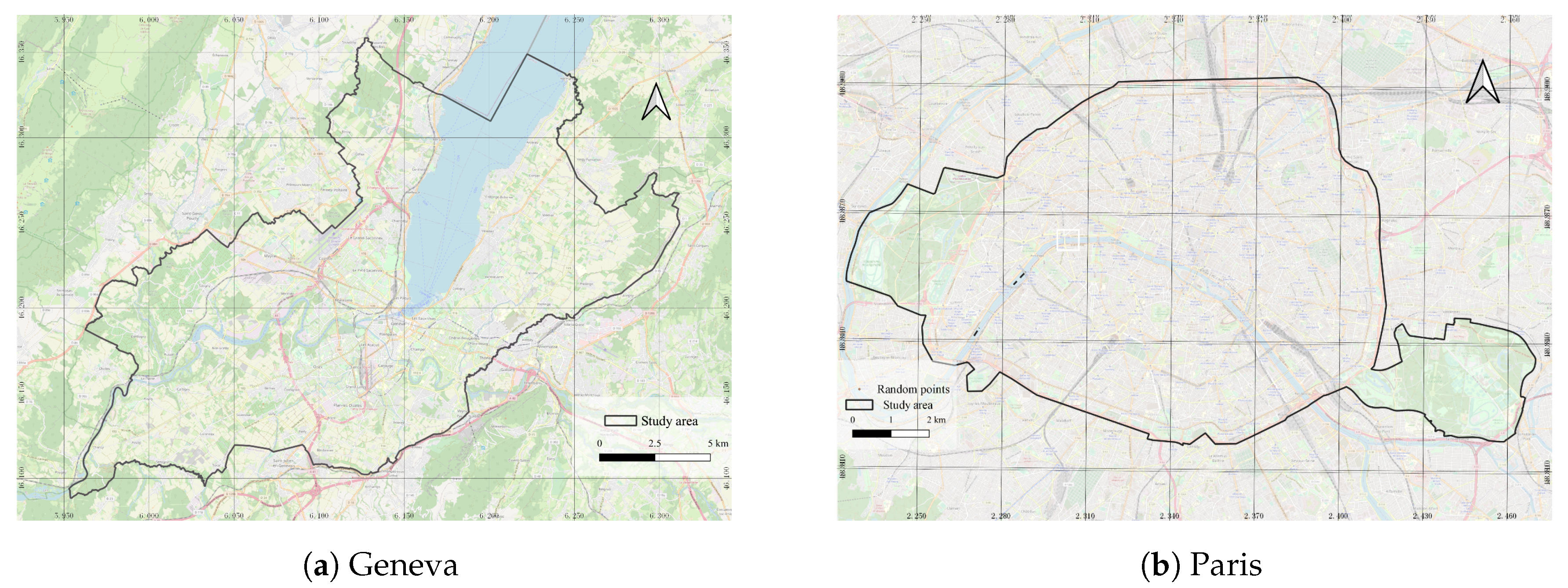
2.1. Study Area
2.2. Datasets
2.2.1. Satellite Imagery
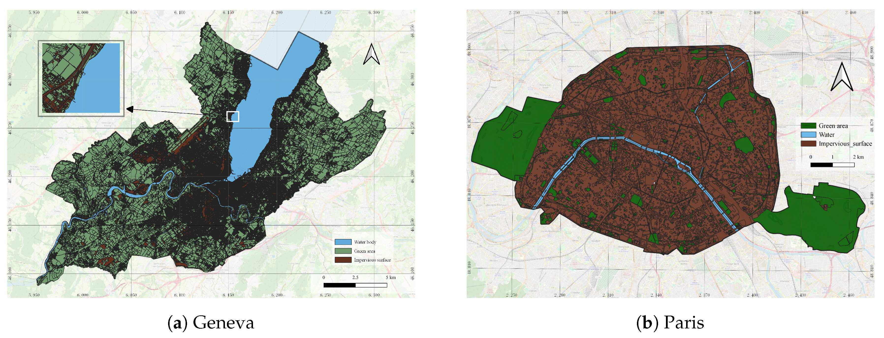
2.2.2. Land Cover Data
2.3. Land Surface Temperature
2.4. NDVI, NDBI and MNDWI Computation
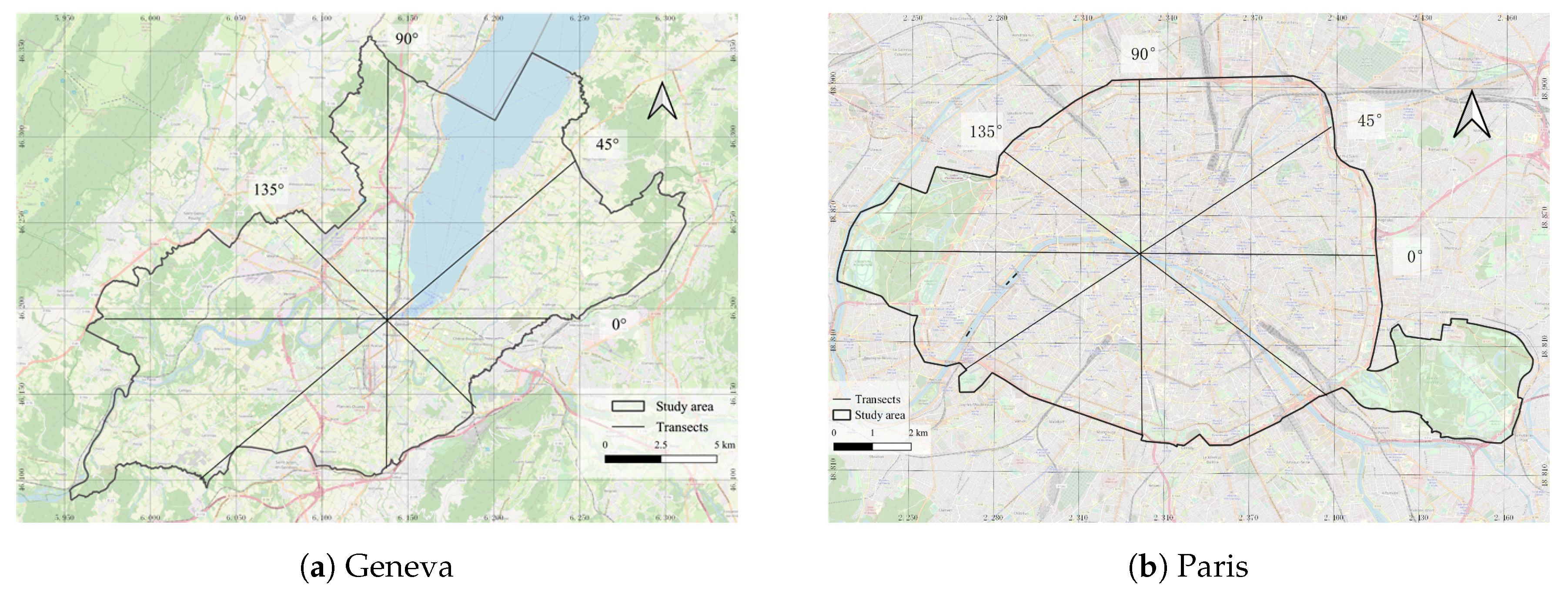
2.5. Distance-Based Analysis
2.6. Grid-Based Analysis
2.7. Point-Based Analysis
3. Results
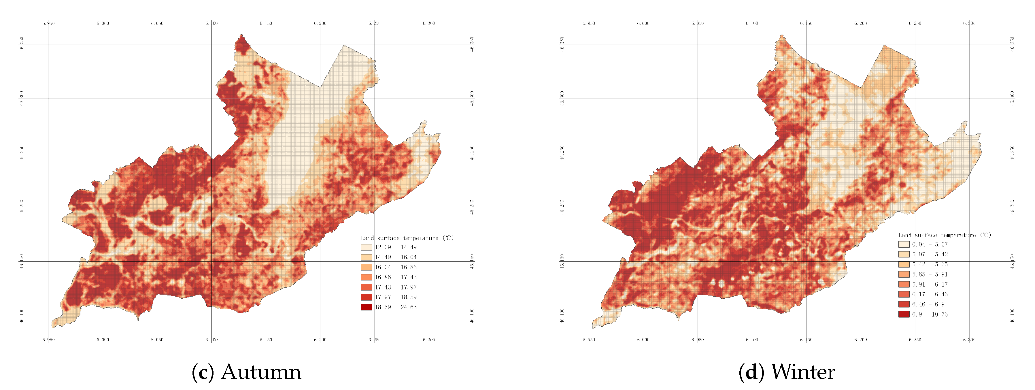
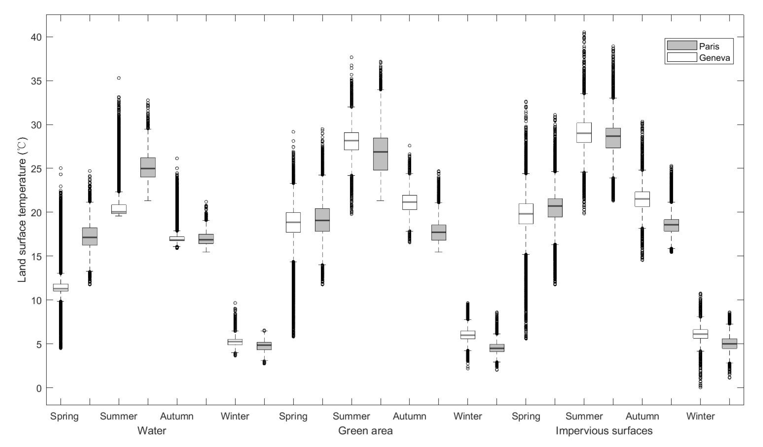
3.1. Land Surface Temperature
3.2. Temporal Distribution of Lst
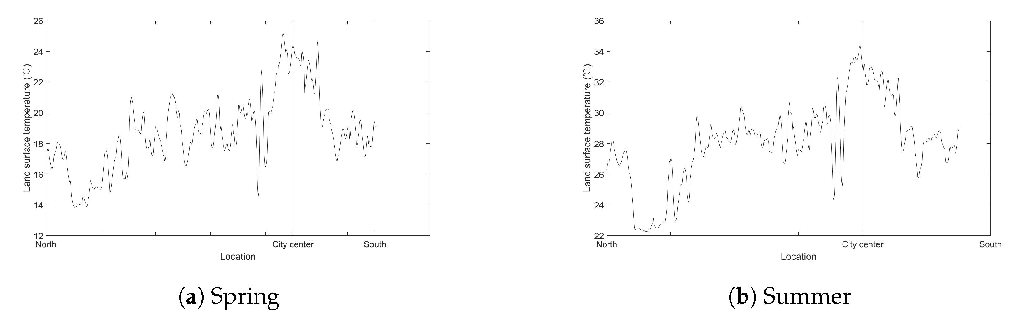
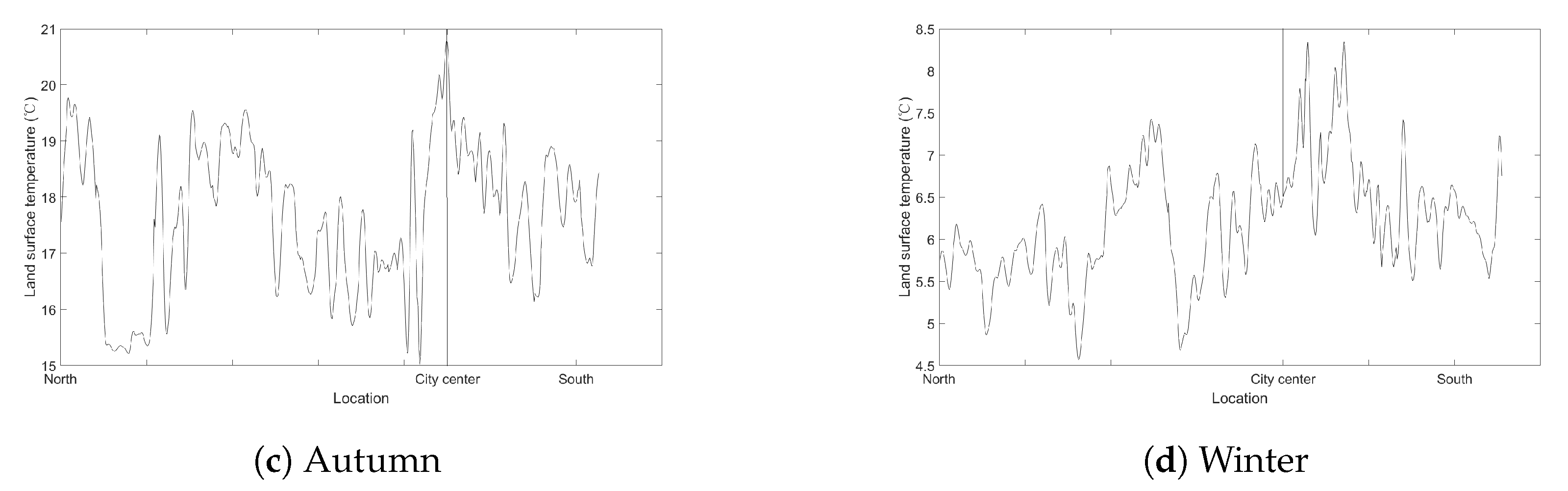
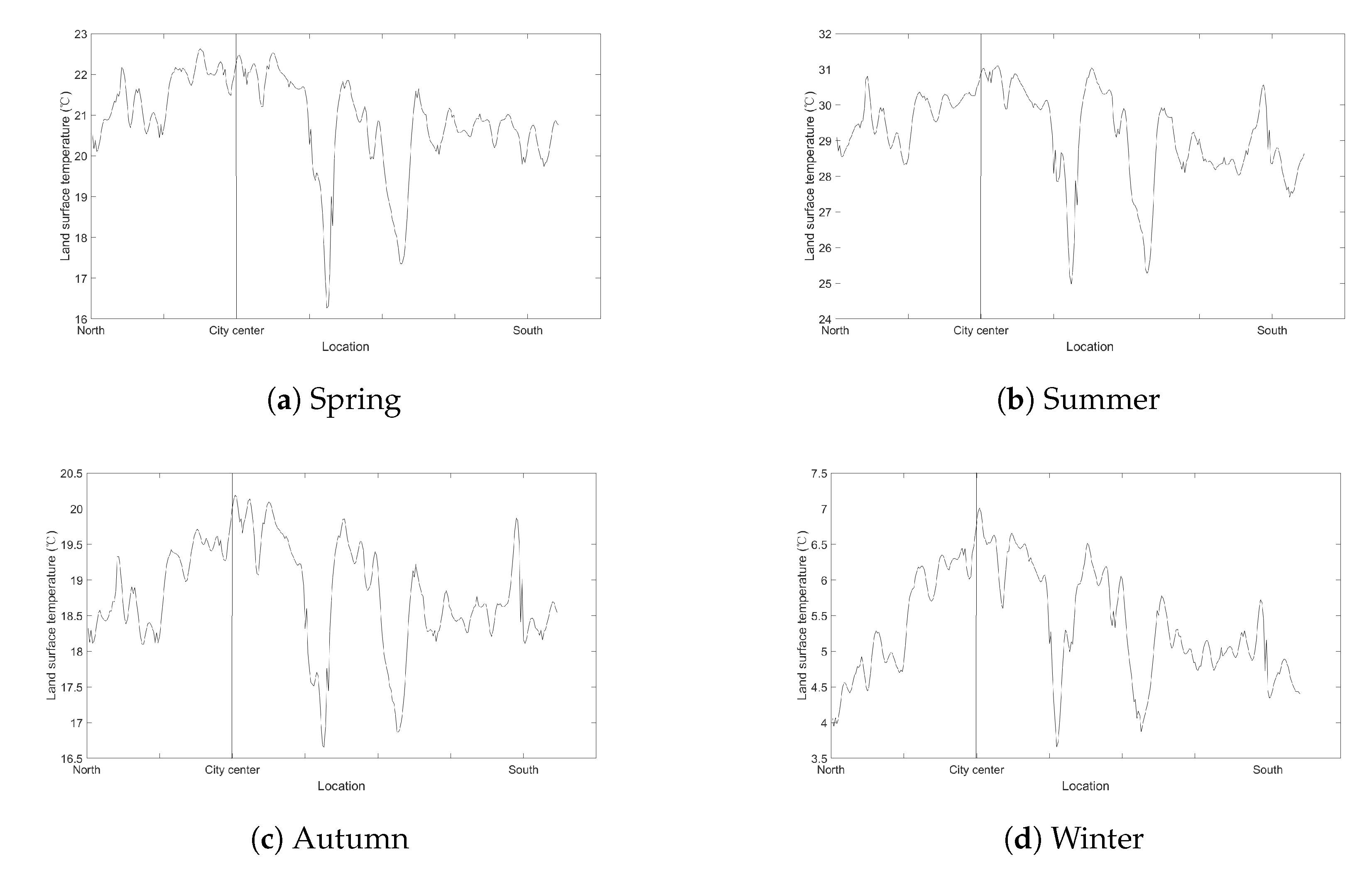
3.3. Distance-Based Results
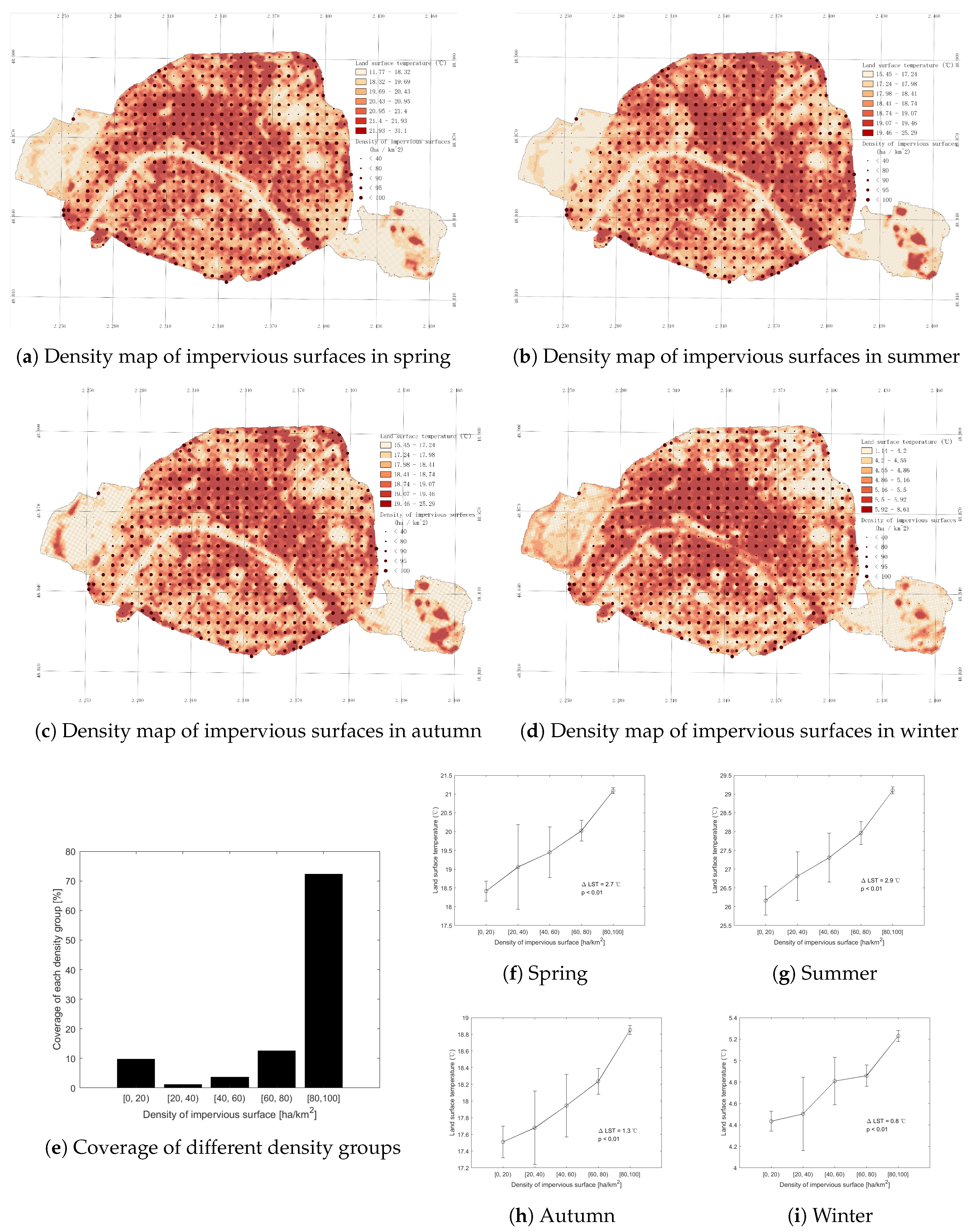
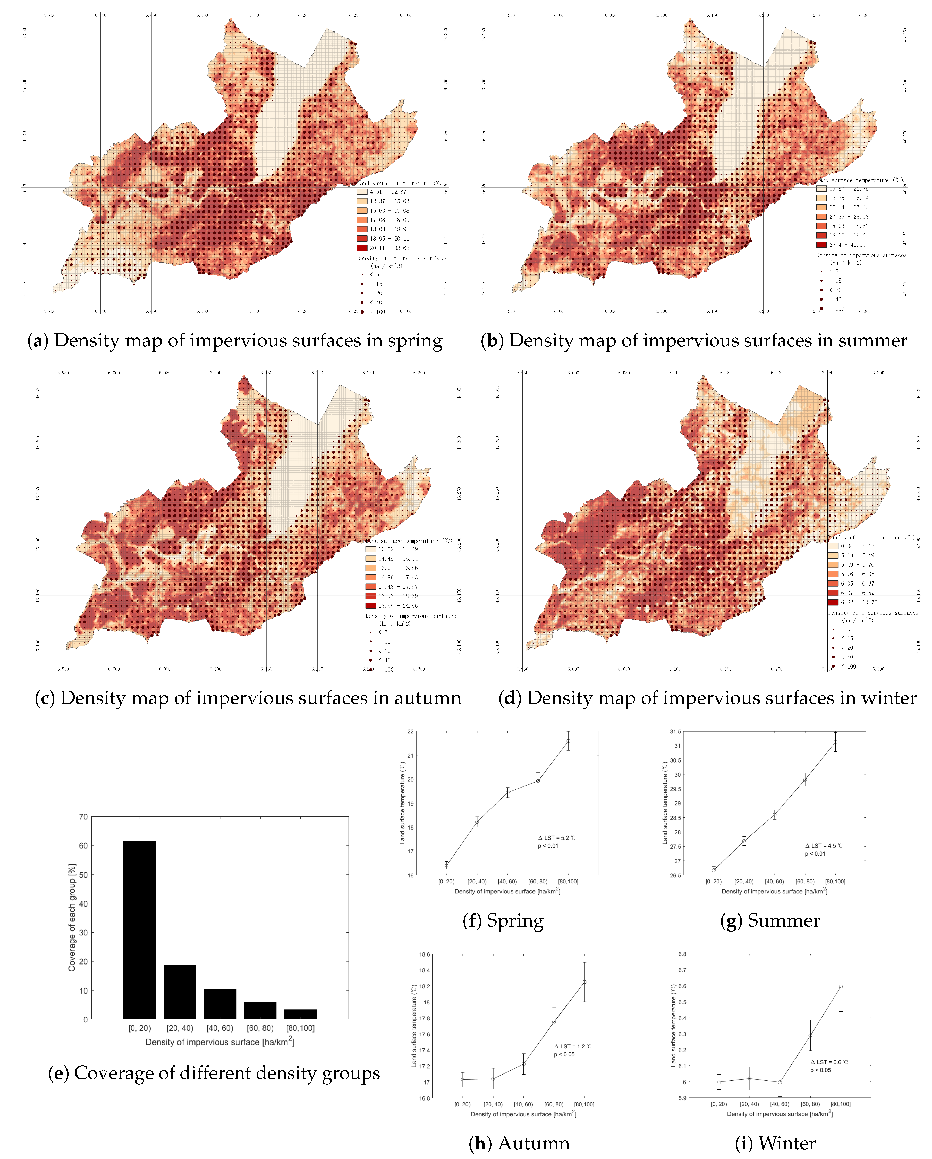
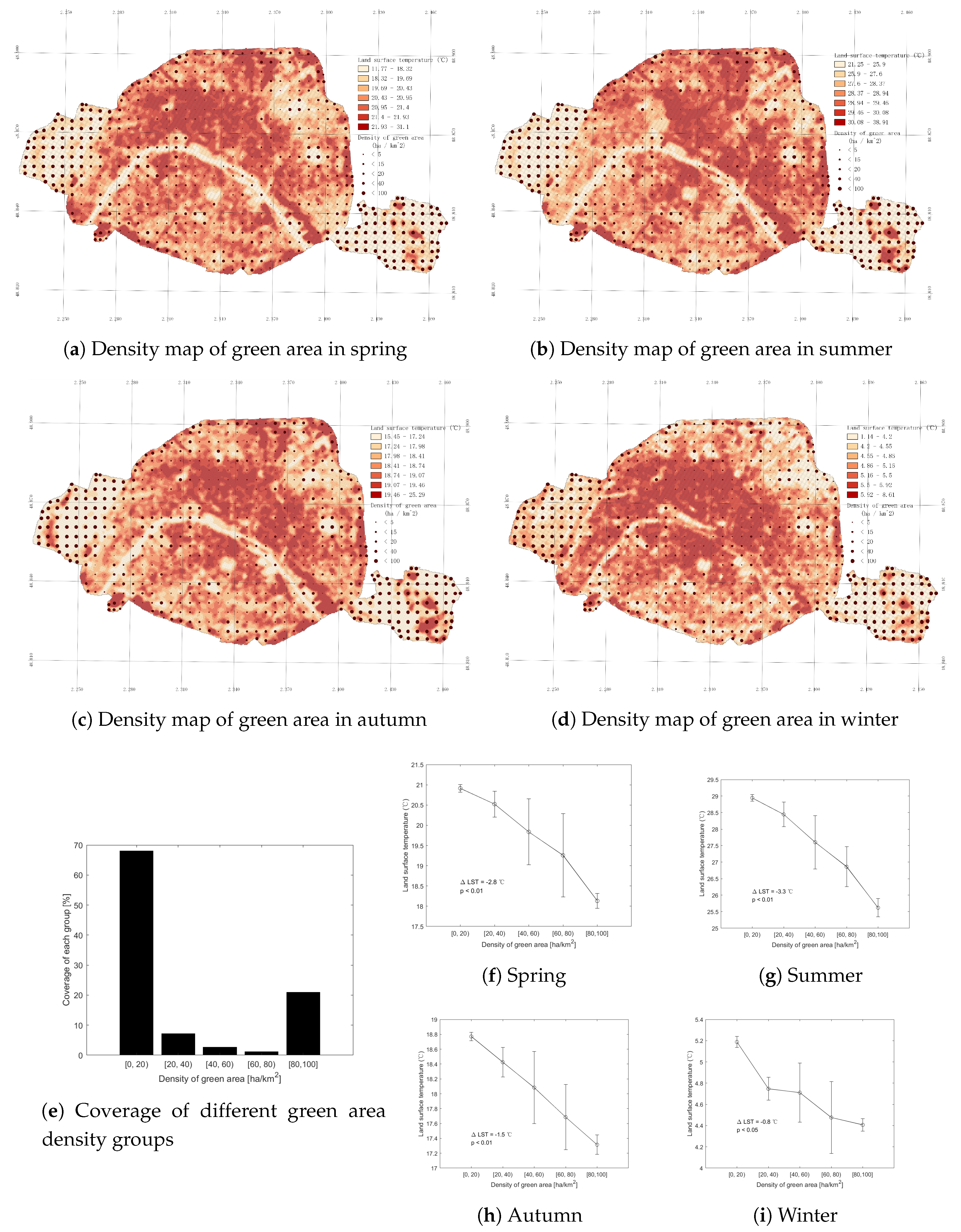
3.4. Grid-Based Results
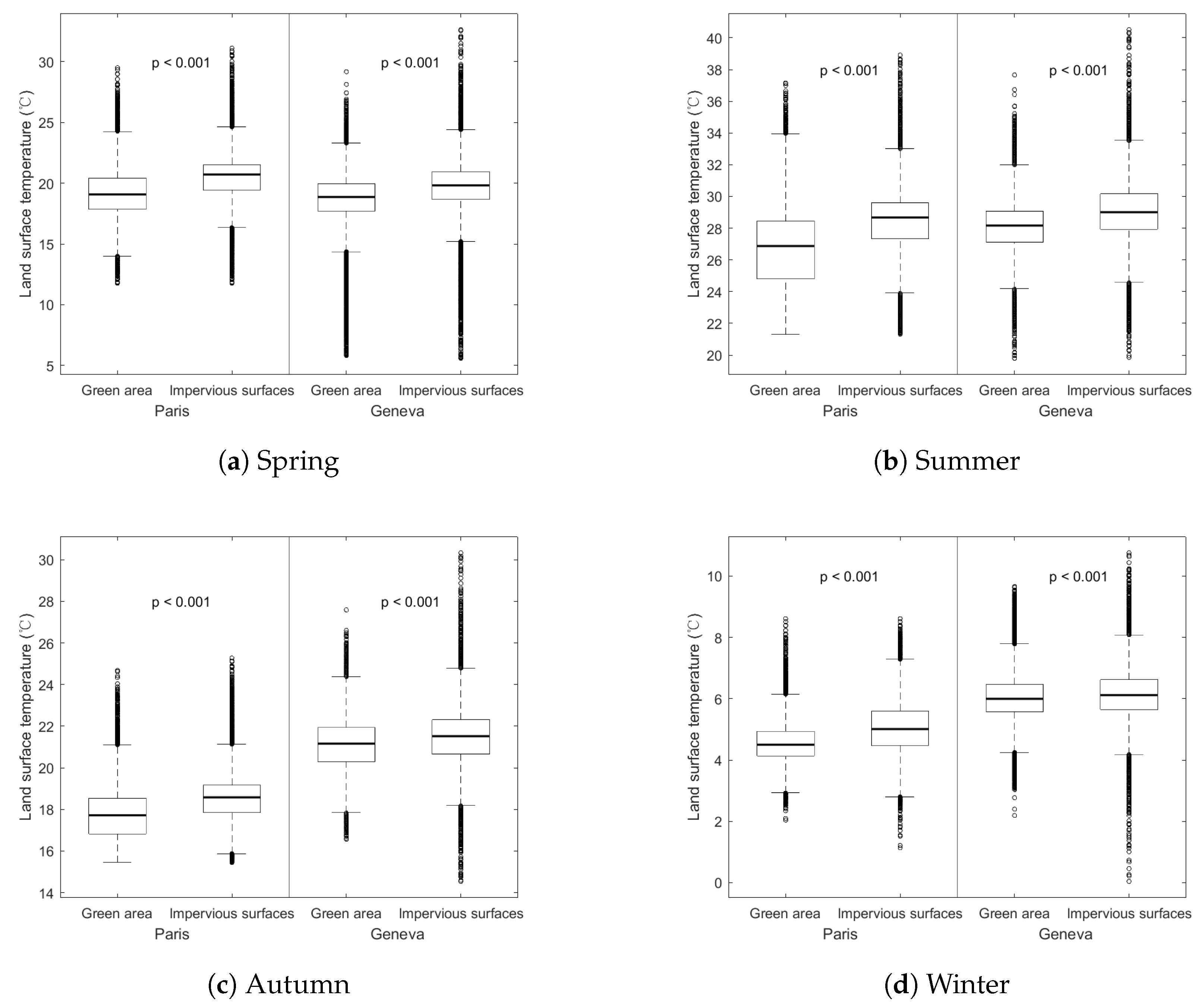
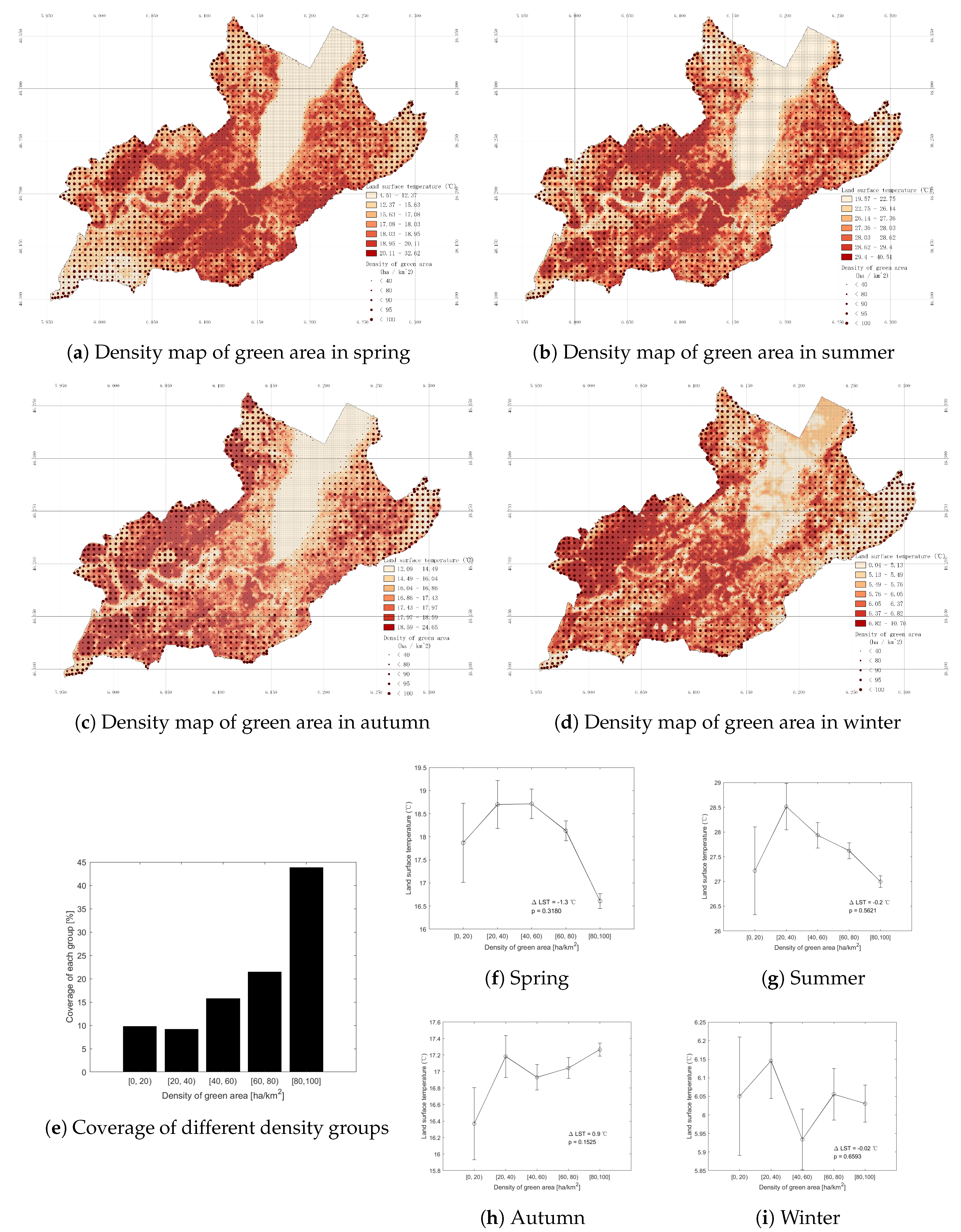
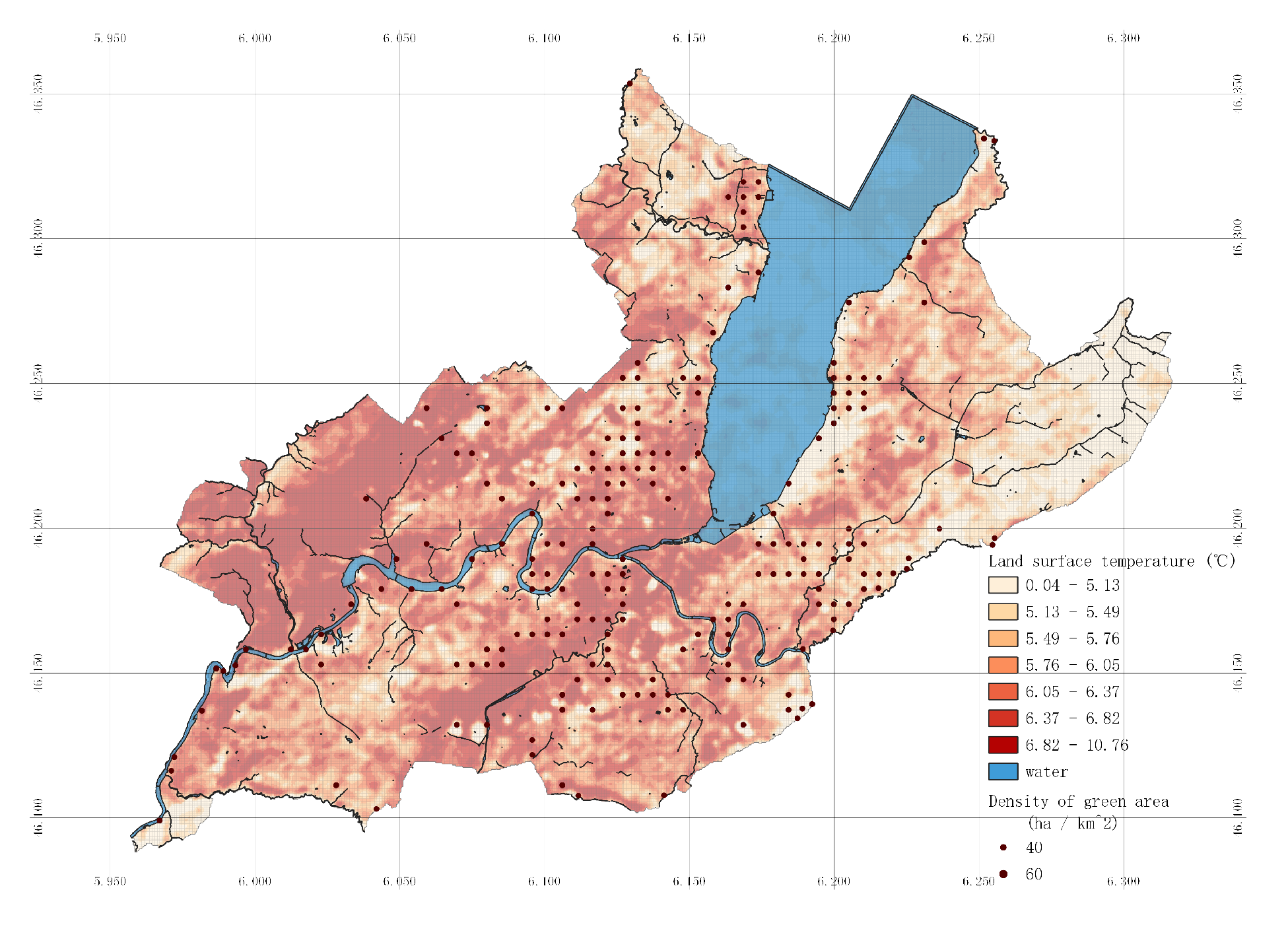
3.5. Point-Based Results
4. Discussion
4.1. Effects of Waterbody on Land Surface Temperature
4.2. Effects of Impervious Surface on Land Surface Temperature
4.3. Effects of Green Area on Land Surface Temperature
4.4. Combined Effects
5. Conclusions
Author Contributions
Funding
Conflicts of Interest
Abbreviations
| LST | Land surface temperature |
| NDBI | the Normalized Difference Built-up Index |
| NDVI | the Normalized Difference Vegetation Index |
| MNDWI | the Modified Normalized Difference Water Index |
| UHI | Urban heat island effects |
| SLM | Spatial lag model |
Appendix A. Tables

| Seasons | Acquisition Date | Collection Category | Day/Night Indicator | Image Quality | Land Cloud Cover | Scene Could Cover |
|---|---|---|---|---|---|---|
| Spring | 2018/5/25 | T1 | Day | 9 | 9.39 | 9.39 |
| 2018/3/22 | T1 | Day | 9 | 4.36 | 4.36 | |
| 2017/5/22 | T1 | Day | 9 | 9.9 | 9.9 | |
| 2017/4/20 | T1 | Day | 9 | 4.43 | 4.43 | |
| 2013/5/27 | T1 | Day | 9 | 7.88 | 7.88 | |
| 2013/4/25 | T1 | Day | 9 | 2.97 | 2.97 | |
| Summer | 2019/6/29 | T1 | Day | 9 | 1.71 | 1.71 |
| 2019/6/13 | T1 | Day | 9 | 3.19 | 3.19 | |
| 2018/6/26 | T1 | Day | 9 | 4.43 | 4.43 | |
| 2017/8/26 | T1 | Day | 9 | 7.04 | 7.04 | |
| 2016/8/23 | T1 | Day | 9 | 0.44 | 0.44 | |
| 2016/8/7 | T1 | Day | 9 | 3.04 | 3.04 | |
| 2015/8/21 | T1 | Day | 9 | 2.47 | 2.47 | |
| 2015/8/5 | T1 | Day | 9 | 0.75 | 0.75 | |
| 2015/7/20 | T1 | Day | 9 | 6.57 | 6.57 | |
| 2015/7/4 | T1 | Day | 9 | 1.77 | 1.77 | |
| 2014/7/17 | T1 | Day | 9 | 1.53 | 1.53 | |
| 2013/8/31 | T1 | Day | 9 | 8.76 | 8.76 | |
| 2013/8/15 | T1 | Day | 9 | 1.01 | 1.01 | |
| 2013/7/14 | T1 | Day | 9 | 3.26 | 3.26 | |
| Autumn | 2019/10/3 | T1 | Day | 9 | 3.24 | 3.24 |
| 2019/9/17 | T1 | Day | 9 | 3.81 | 3.81 | |
| 2017/10/13 | T1 | Day | 9 | 6.66 | 6.66 | |
| 2016/9/24 | T1 | Day | 9 | 6.19 | 6.19 | |
| 2016/9/8 | T1 | Day | 9 | 2.17 | 2.17 | |
| 2014/11/22 | T1 | Day | 9 | 9.95 | 9.95 | |
| Winter | 2020/2/24 | T1 | Day | 9 | 7.88 | 7.88 |
| 2019/2/21 | T1 | Day | 9 | 1.86 | 1.86 | |
| 2019/2/5 | T1 | Day | 9 | 3.58 | 3.58 | |
| 2019/1/4 | T1 | Day | 9 | 7.02 | 7.02 |
| Seasons | Acquisition Date | Collection Category | Day/Night Indicator | Image Quality | Land Cloud Cover | Scene Could Cover |
|---|---|---|---|---|---|---|
| Spring | 2020/5/19 | T1 | Day | 9 | 0.27 | 0.27 |
| 2020/4/1 | T1 | Day | 9 | 0.01 | 0.01 | |
| 2019/3/30 | T1 | Day | 9 | 9.42 | 9.42 | |
| 2017/4/9 | T1 | Day | 9 | 0.01 | 0.01 | |
| 2015/4/20 | T1 | Day | 9 | 5.99 | 5.99 | |
| 2014/5/19 | T1 | Day | 9 | 0.1 | 0.1 | |
| 2014/4/17 | T1 | Day | 9 | 5.66 | 5.66 | |
| 2014/3/16 | T1 | Day | 9 | 8.18 | 8.18 | |
| Summer | 2019/7/4 | T1 | Day | 9 | 0 | 0 |
| 2019/6/2 | T1 | Day | 9 | 0.13 | 0.13 | |
| 2018/8/2 | T1 | Day | 9 | 2.82 | 2.82 | |
| 2015/6/7 | T1 | Day | 9 | 9.58 | 9.58 | |
| 2013/8/20 | T1 | Day | 9 | 4.99 | 4.99 | |
| 2013/7/19 | T1 | Day | 9 | 9.59 | 9.59 | |
| Autumn | 2019/9/6 | T1 | Day | 9 | 7.73 | 7.73 |
| 2018/10/21 | T1 | Day | 9 | 0.06 | 0.06 | |
| 2018/10/5 | T1 | Day | 9 | 0.04 | 0.04 | |
| 2016/10/31 | T1 | Day | 9 | 0.03 | 0.03 | |
| 2015/9/27 | T1 | Day | 9 | 8.76 | 8.76 | |
| 2014/11/11 | T1 | Day | 9 | 4.55 | 4.55 | |
| 2014/9/8 | T1 | Day | 9 | 2.36 | 2.36 | |
| 2014/9/8 | T1 | Day | 9 | 2.36 | 2.36 | |
| 2013/9/5 | T1 | Day | 9 | 0.01 | 0.01 | |
| Winter | 2019/2/26 | T1 | Day | 9 | 0.04 | 0.04 |
| 2018/2/23 | T1 | Day | 9 | 0.15 | 0.15 | |
| 2017/1/19 | T1 | Day | 9 | 3.42 | 3.42 | |
| 2013/12/10 | T1 | Day | 9 | 8.95 | 8.95 |
| Statistics | Lower Outlier | Q1 | Median | Q3 | Upper Outlier | IQR | SD | |
|---|---|---|---|---|---|---|---|---|
| Water | Spring | 13.25 | 16.23 | 17.14 | 18.22 | 21.20 | 1.99 | 1.64 |
| Summer | 20.68 | 24.00 | 24.99 | 26.22 | 29.54 | 2.22 | 1.71 | |
| Autumn | 14.83 | 16.43 | 16.87 | 17.49 | 19.09 | 1.07 | 0.82 | |
| Winter | 3.04 | 4.32 | 4.86 | 5.18 | 6.47 | 0.86 | 0.60 | |
| Green area | Spring | 13.99 | 17.84 | 19.07 | 20.41 | 24.27 | 2.57 | 1.79 |
| Summer | 19.30 | 24.79 | 26.88 | 28.46 | 33.96 | 3.67 | 2.31 | |
| Autumn | 14.25 | 16.83 | 17.72 | 18.54 | 21.11 | 1.72 | 1.13 | |
| Winter | 2.93 | 4.13 | 4.50 | 4.94 | 6.15 | 0.81 | 0.63 | |
| Impervious surface | Spring | 16.34 | 19.45 | 20.72 | 21.52 | 24.63 | 2.07 | 1.72 |
| Summer | 23.92 | 27.33 | 28.67 | 29.60 | 33.01 | 2.27 | 2.05 | |
| Autumn | 15.87 | 17.85 | 18.58 | 19.16 | 21.14 | 1.32 | 1.06 | |
| Winter | 2.80 | 4.48 | 5.01 | 5.60 | 7.28 | 1.12 | 0.76 | |
| Satistics | Lower Outlier | Q1 | Median | Q3 | Upper Outlier | IQR | SD | |
|---|---|---|---|---|---|---|---|---|
| Water | Spring | 9.84 | 11.04 | 11.29 | 11.84 | 13.03 | 0.80 | 1.86 |
| Summer | 18.35 | 19.85 | 20.05 | 20.85 | 22.35 | 1.00 | 1.94 | |
| Autumn | 16.09 | 16.76 | 16.86 | 17.21 | 17.88 | 0.45 | 1.06 | |
| Winter | 4.00 | 4.92 | 5.26 | 5.54 | 6.46 | 0.62 | 0.55 | |
| Green area | Spring | 14.36 | 17.72 | 18.86 | 19.95 | 23.30 | 2.24 | 2.05 |
| Summer | 24.19 | 27.12 | 28.16 | 29.07 | 32.00 | 1.95 | 1.56 | |
| Autumn | 17.85 | 20.30 | 21.16 | 21.93 | 24.39 | 1.64 | 1.23 | |
| Winter | 4.25 | 5.57 | 5.99 | 6.46 | 7.79 | 0.89 | 0.72 | |
| Impervious surface | Spring | 15.20 | 18.65 | 19.82 | 20.95 | 24.41 | 2.30 | 2.11 |
| Summer | 24.57 | 27.93 | 29.01 | 30.17 | 33.53 | 2.24 | 1.85 | |
| Autumn | 18.18 | 20.66 | 21.52 | 22.32 | 24.80 | 1.65 | 1.32 | |
| Winter | 4.18 | 5.65 | 6.12 | 6.62 | 8.08 | 0.98 | 0.76 | |
References
- Nations, U. 68% of the World Population Projected to Live in Urban Areas by 2050, Says UN. 2018. Available online: www.un.org (accessed on 30 September 2020).
- Song, J.; Chen, W.; Zhang, J.; Huang, K.; Hou, B.; Prishchepov, A.V. Effects of building density on land surface temperature in China: Spatial patterns and determinants. Landsc. Urban Plan. 2020, 198, 103794. [Google Scholar] [CrossRef]
- Mauree, D.; Naboni, E.; Coccolo, S.; Perera, A.T.D.; Nik, V.M.; Scartezzini, J.L. A review of assessment methods for the urban environment and its energy sustainability to guarantee climate adaptation of future cities. Renew. Sustain. Energy Rev. 2019, 112, 733–746. [Google Scholar] [CrossRef]
- Norton, B.A.; Coutts, A.M.; Livesley, S.J.; Harris, R.J.; Hunter, A.M.; Williams, N.S.G. Planning for cooler cities: A framework to prioritise green infrastructure to mitigate high temperatures in urban landscapes. Landsc. Urban Plan. 2015, 134, 127–138. [Google Scholar] [CrossRef]
- Langemeyer, J.; Wedgwood, D.; McPhearson, T.; Baró, F.; Madsen, A.L.; Barton, D.N. Creating urban green infrastructure where it is needed—A spatial ecosystem service-based decision analysis of green roofs in Barcelona. Sci. Total. Environ. 2020, 707, 135487. [Google Scholar] [CrossRef] [PubMed]
- Fu, W.; Ma, J.; Chen, P.; Chen, F. Remote Sensing Satellites for Digital Earth. In Manual of Digital Earth; Guo, H., Goodchild, M.F., Annoni, A., Eds.; Springer: Singapore, 2020; pp. 55–123. [Google Scholar] [CrossRef] [Green Version]
- Guo, H.D.; Zhang, L.; Zhu, L.W. Earth observation big data for climate change research. Adv. Clim. Chang. Res. 2015, 6, 108–117. [Google Scholar] [CrossRef]
- Yu, X.; Guo, X.; Wu, Z. Land Surface Temperature Retrieval from Landsat 8 TIRS—Comparison between Radiative Transfer Equation-Based Method, Split Window Algorithm and Single Channel Method. Remote Sens. 2014, 6, 9829–9852. [Google Scholar] [CrossRef] [Green Version]
- Kumar, D.; Shekhar, S. Statistical analysis of land surface temperature–vegetation indexes relationship through thermal remote sensing. Ecotoxicol. Environ. Saf. 2015, 121, 39–44. [Google Scholar] [CrossRef]
- Weng, Q.; Fu, P. Modeling annual parameters of clear-sky land surface temperature variations and evaluating the impact of cloud cover using time series of Landsat TIR data. Remote Sens. Environ. 2014, 140, 267–278. [Google Scholar] [CrossRef]
- Bokaie, M.; Zarkesh, M.K.; Arasteh, P.D.; Hosseini, A. Assessment of Urban Heat Island based on the relationship between land surface temperature and Land Use/ Land Cover in Tehran. Sustain. Cities Soc. 2016, 23, 94–104. [Google Scholar] [CrossRef]
- Zhou, W.; Huang, G.; Cadenasso, M.L. Does spatial configuration matter? Understanding the effects of land cover pattern on land surface temperature in urban landscapes. Landsc. Urban Plan. 2011, 102, 54–63. [Google Scholar] [CrossRef]
- Zhang, Y.; Odeh, I.O.A.; Han, C. Bi-temporal characterization of land surface temperature in relation to impervious surface area, NDVI and NDBI, using a sub-pixel image analysis. Int. J. Appl. Earth Obs. Geoinf. 2009, 11, 256–264. [Google Scholar] [CrossRef]
- Estoque, R.; Murayama, Y.; Myint, S. Effects of landscape composition and pattern on land surface temperature: An urban heat island study in the megacities of Southeast Asia. Sci. Total. Environ. 2016, 577, 349–359. [Google Scholar] [CrossRef] [PubMed]
- Zhang, X.; Estoque, R.C.; Murayama, Y. An urban heat island study in Nanchang City, China based on land surface temperature and social-ecological variables. Sustain. Cities Soc. 2017, 32, 557–568. [Google Scholar] [CrossRef]
- Office, F.S. Geneva. 2020. Available online: www.bfs.admin.ch (accessed on 30 September 2020).
- Tourist office, P. Climate in Paris–Paris Tourist Office; Paris Tourist Office: Paris, France, 2020. [Google Scholar]
- Region, I.P. Portail Open Data de L’Institut Paris Region. 2020. Available online: data-iau-idf.opendata.arcgis.com (accessed on 30 September 2020).
- Data, P. Home—Paris Data. 2020. Available online: https://opendata.paris.fr/pages/home/ (accessed on 30 September 2020).
- SITG. Catalog | SITG. 2020. Available online: https://ge.ch/sitg/ (accessed on 30 September 2020).
- Avdan, U.; Jovanovska, G. Algorithm for Automated Mapping of Land Surface Temperature Using LANDSAT 8 Satellite Data. J. Sens. 2016, 2016, 1–8. [Google Scholar] [CrossRef] [Green Version]
- Peng, J.; Jia, J.; Liu, Y.; Li, H.; Wu, J. Seasonal contrast of the dominant factors for spatial distribution of land surface temperature in urban areas. Remote Sens. Environ. 2018, 215, 255–267. [Google Scholar] [CrossRef]
- Yuan, F.; Bauer, M.E. Comparison of impervious surface area and normalized difference vegetation index as indicators of surface urban heat island effects in Landsat imagery. Remote Sens. Environ. 2007, 106, 375–386. [Google Scholar] [CrossRef]
- USGS. NDVI, the Foundation for Remote Sensing Phenology; 2020. Available online: https://www.usgs.gov/land-resources/eros/phenology/science/ndvi-foundation-remote-sensing-phenology (accessed on 30 September 2020).
- Zha, Y.; Gao, J.; Ni, S. Use of normalized difference built-up index in automatically mapping urban areas from TM imagery. Int. J. Remote Sens. 2003, 24, 583–594. [Google Scholar] [CrossRef]
- Xu, H. A study on information extraction of waterbody with the modified normalized difference water index (MNDWI). J. Remote Sens. 2005, 9, 589–595. [Google Scholar]
- Xu, H. Modification of normalised difference water index (NDWI) to enhance open water features in remotely sensed imagery. Int. J. Remote Sens. 2006, 27, 3025–3033. [Google Scholar] [CrossRef]
- Qiao, R.; Liu, T. Impact of building greening on building energy consumption: A quantitative computational approach. J. Clean. Prod. 2020, 246, 119020. [Google Scholar] [CrossRef]
- Anselin, L. Spatial Weights as Distance Functions. 2018. Available online: https://geodacenter.github.io/workbook/4c_distance_functions/lab4c.html#inverse-distance-weights (accessed on 30 September 2020).
- Pal, S.; Ziaul, S. Detection of land use and land cover change and land surface temperature in English Bazar urban centre. Egypt. J. Remote Sens. Space Sci. 2017, 20, 125–145. [Google Scholar] [CrossRef] [Green Version]
- Huang, L.; Zhao, D.; Wang, J.; Zhu, J.; Li, J. Scale impacts of land cover and vegetation corridors on urban thermal behavior in Nanjing, China. Theor. Appl. Climatol. 2008, 94, 241–257. [Google Scholar] [CrossRef]
- Maimaitiyiming, M.; Ghulam, A.; Tiyip, T.; Pla, F.; Latorre-Carmona, P.; Halik, u.; Sawut, M.; Caetano, M. Effects of green space spatial pattern on land surface temperature: Implications for sustainable urban planning and climate change adaptation. ISPRS J. Photogramm. Remote Sens. 2014, 89, 59–66. [Google Scholar] [CrossRef] [Green Version]
- Naeem, S.; Cao, C.; Waqar, M.M.; Wei, C.; Acharya, B.K. Vegetation role in controlling the ecoenvironmental conditions for sustainable urban environments: A comparison of Beijing and Islamabad. J. Appl. Remote Sens. 2018, 12, 16013. [Google Scholar] [CrossRef] [Green Version]
- Li, X.; Zhou, W.; Ouyang, Z.; Xu, W.; Zheng, H. Spatial pattern of greenspace affects land surface temperature: Evidence from the heavily urbanized Beijing metropolitan area, China. Landsc. Ecol. 2012, 27, 887–898. [Google Scholar] [CrossRef]
- Zhang, X.; Zhong, T.; Feng, X.; Wang, K. Estimation of the relationship between vegetation patches and urban land surface temperature with remote sensing. Int. J. Remote Sens. 2009, 30, 2105–2118. [Google Scholar] [CrossRef]
- Inventory, T.N.F. Insights into the Swiss Forest; Technical Report. National Forest Inventory, 2011. Available online: www.lfi.ch (accessed on 30 September 2020).
- Wang, Y. Encyclopedia of Natural Resources–Land–Volume I; Google-Books-ID: UZDUDwAAQBAJ; CRC Press: Boca Raton, FL, USA, 2014. [Google Scholar]
- Kim, Y.; Still, C.J.; Hanson, C.V.; Kwon, H.; Greer, B.T.; Law, B.E. Canopy skin temperature variations in relation to climate, soil temperature, and carbon flux at a ponderosa pine forest in central Oregon. Agric. For. Meteorol. 2016, 226–227, 161–173. [Google Scholar] [CrossRef] [Green Version]
- Uchida, M.; Mo, W.; Nakatsubo, T.; Tsuchiya, Y.; Horikoshi, T.; Koizumi, H. Microbial activity and litter decomposition under snow cover in a cool-temperate broad-leaved deciduous forest. Agric. For. Meteorol. 2005, 134, 102–109. [Google Scholar] [CrossRef]
- Qiu, S.; McComb, A.; Bell, R.; Davis, J. Response of soil microbial activity to temperature, moisture, and litter leaching on a wetland transect during seasonal refilling. Wetl. Ecol. Manag. 2005, 13, 43–54. [Google Scholar] [CrossRef]
- Hu, Y.; Dai, Z.; Guldmann, J.M. Modeling the impact of 2D/3D urban indicators on the urban heat island over different seasons: A boosted regression tree approach. J. Environ. Manag. 2020, 266, 110424. [Google Scholar] [CrossRef]
- Chun, B.; Guldmann, J.M. Impact of greening on the urban heat island: Seasonal variations and mitigation strategies. Comput. Environ. Urban Syst. 2018, 71, 165–176. [Google Scholar] [CrossRef]
- Mushore, T.D.; Mutanga, O.; Odindi, J.; Dube, T. Linking major shifts in land surface temperatures to long term land use and land cover changes: A case of Harare, Zimbabwe. Urban Clim. 2017, 20, 120–134. [Google Scholar] [CrossRef]
- Rasul, A.; Balzter, H.; Smith, C. Spatial variation of the daytime Surface Urban Cool Island during the dry season in Erbil, Iraqi Kurdistan, from Landsat 8. Urban Clim. 2015, 14, 176–186. [Google Scholar] [CrossRef] [Green Version]
- Grilo, F.; Pinho, P.; Aleixo, C.; Catita, C.; Silva, P.; Lopes, N.; Freitas, C.; Santos-Reis, M.; McPhearson, T.; Branquinho, C. Using green to cool the grey: Modelling the cooling effect of green spaces with a high spatial resolution. Sci. Total. Environ. 2020, 724, 138182. [Google Scholar] [CrossRef] [PubMed]
- Weather, B. Geneva. 2020. Available online: www.bbc.com (accessed on 30 September 2020).
- Gao, B.C. NDWI—A normalized difference water index for remote sensing of vegetation liquid water from space. Remote Sens. Environ. 1996, 58, 257–266. [Google Scholar] [CrossRef]
- Mathew, A.; Khandelwal, S.; Kaul, N. Investigating spatial and seasonal variations of urban heat island effect over Jaipur city and its relationship with vegetation, urbanization and elevation parameters. Sustain. Cities Soc. 2017, 35, 157–177. [Google Scholar] [CrossRef]
- Ogashawara, I.; Bastos, V.D.S.B. A Quantitative Approach for Analyzing the Relationship between Urban Heat Islands and Land Cover. Remote Sens. 2012, 4, 3596–3618. [Google Scholar] [CrossRef] [Green Version]
- Dong, J.; Lin, M.; Zuo, J.; Lin, T.; Liu, J.; Sun, C.; Luo, J. Quantitative study on the cooling effect of green roofs in a high-density urban Area—A case study of Xiamen, China. J. Clean. Prod. 2020, 255, 120152. [Google Scholar] [CrossRef]
- Ren, Y.; Deng, L.Y.; Zuo, S.D.; Song, X.D.; Liao, Y.L.; Xu, C.D.; Chen, Q.; Hua, L.Z.; Li, Z.W. Quantifying the influences of various ecological factors on land surface temperature of urban forests. Environ. Pollut. 2016, 216, 519–529. [Google Scholar] [CrossRef] [Green Version]
- Du, Z.; Zhang, X.; Xu, X.; Zhang, H.; Wu, Z.; Pang, J. Quantifying influences of physiographic factors on temperate dryland vegetation, Northwest China. Sci. Rep. 2017, 7, 40092. [Google Scholar] [CrossRef]
- Weng, Q.; Lu, D.; Schubring, J. Estimation of land surface temperature–vegetation abundance relationship for urban heat island studies. Remote Sens. Environ. 2004, 89, 467–483. [Google Scholar] [CrossRef]


| Class | Percentage (%) | Reclassified Groups | Source |
|---|---|---|---|
| Standing water, stream and reed bed | 14.75 | Water | SITG * |
| Buildings | 5.07 | ||
| Coated surfaces | 13.43 | Impervious surfaces | |
| Surfaces without vegetation | 0.82 | ||
| Wooded areas | 15.04 | Green area | |
| Green surfaces | 50.89 |
| Class | Percentage (%) | Reclassified Groups | Source |
|---|---|---|---|
| Water | 2.50 | Water | |
| Housing | 39.02 | Impervious surfaces | Institut Paris Region * |
| Activities | 6.73 | ||
| Equipment | 12.22 | ||
| Transports | 13.71 | ||
| Artificial open spaces | 17.72 | ||
| Quarries, landfills, construction sites | 0.57 | ||
| Wood or forest | 7.34 | Green area | |
| Semi-natural | 0.04 | Institut Paris Region * | |
| Agricultural space | 0.16 | Paris data ** |
| Coefficients | ||||||||
|---|---|---|---|---|---|---|---|---|
| Variables | Paris | Geneva | ||||||
| Spring | Summer | Autumn | Winter | Spring | Summer | Autumn | Winter | |
| WLST | 0.8858 | 0.8949 | 0.8966 | 0.9380 | 0.9205 | 0.9629 | 0.8541 | 0.9440 |
| Constant | 2.5820 | 3.2062 | 2.1065 | 0.3843 | 1.6081 | 0.9629 | 2.1065 | 0.1696 |
| NDBI | −9.5530 | −4.3836 | −4.1051 | −3.4244 | 1.6134 | 2.9515 | −2.5516 | 6.2503 |
| MNDWI | −11.9005 | −8.1810 | −6.5245 | −3.5342 | −5.2034 | −6.2199 | −8.6041 | 3.7929 |
| NDVI | −11.4616 | −7.2408 | −5.8174 | −3.8537 | −2.1090 | −2.5941 | −5.8284 | 5.6238 |
| R | 0.8640 | 0.8982 | 0.8425 | 0.8192 | 0.9624 | 0.9629 | 0.9593 | 0.8913 |
© 2020 by the authors. Licensee MDPI, Basel, Switzerland. This article is an open access article distributed under the terms and conditions of the Creative Commons Attribution (CC BY) license (http://creativecommons.org/licenses/by/4.0/).
Share and Cite
Ge, X.; Mauree, D.; Castello, R.; Scartezzini, J.-L. Spatio-Temporal Relationship between Land Cover and Land Surface Temperature in Urban Areas: A Case Study in Geneva and Paris. ISPRS Int. J. Geo-Inf. 2020, 9, 593. https://0-doi-org.brum.beds.ac.uk/10.3390/ijgi9100593
Ge X, Mauree D, Castello R, Scartezzini J-L. Spatio-Temporal Relationship between Land Cover and Land Surface Temperature in Urban Areas: A Case Study in Geneva and Paris. ISPRS International Journal of Geo-Information. 2020; 9(10):593. https://0-doi-org.brum.beds.ac.uk/10.3390/ijgi9100593
Chicago/Turabian StyleGe, Xu, Dasaraden Mauree, Roberto Castello, and Jean-Louis Scartezzini. 2020. "Spatio-Temporal Relationship between Land Cover and Land Surface Temperature in Urban Areas: A Case Study in Geneva and Paris" ISPRS International Journal of Geo-Information 9, no. 10: 593. https://0-doi-org.brum.beds.ac.uk/10.3390/ijgi9100593