A New Urban Vitality Analysis and Evaluation Framework Based on Human Activity Modeling Using Multi-Source Big Data

Abstract

A quantitative study of urban vitality brings new insights for evaluating the external construction environment and internal development power of cities. However, it still has limited knowledge of the relations between people’s diverse urban life and urban vitality, although urban activities are often used as the proxy for urban vitality. This paper aims to deeply mine the content of urban social life and reveal the driving mechanism of urban vitality after inspecting human activities. We propose a general framework for exploring the spatial pattern and driving mechanism of urban vitality using multi-source big data. It builds a mapping relationship between various urban activities and urban vitality aspects, including economic and social. In addition, the physical environment (static) and human–land interaction (dynamic) indicators are designed to analyze the driving mechanism of urban vitality using the Geographically Weighted Regression model. The results show that the spatial pattern and driving factors of urban vitality are heterogeneous over space regarding both the economic and social aspects of our experimental study. This work provides us with multiple perspectives to understand the connotation of urban vitality and urges us to develop rational strategies to make the city more vital, coordinated, and sustainable.

1. Introduction

Creating a vibrant city is an essential goal of urban development [1]. How to effectively evaluate the abstract concepts and connotations of urban vitality has always been a concern of urbanists, sociologists, and urban planners. With the development of geospatial information science and the emergence of new data sources, spatial big data mining and GIS (Geographic Information System) analysis techniques have been successfully applied to quantitative evaluation of urban vitality [2,3]. According to the previous studies [4,5], urban morphology quantified by some spatial metrics can be used to infer urban functions. Good cities tend to be a balance of a reasonably ordered and legible city form [6]. Hence, the quantitative evaluation methods assess the differences in urban construction, spatial design, and urban development within a city and among different cities [6,7]. The relationship between landscape characteristics and urban vibrancy has also been discussed [8,9]. They all have provided reference opinions for urban planning practice. Based on theory study and field investigation, the dynamic interaction between human and urban space is considered the source of spatial vitality [10]. Nevertheless, it is insufficient to study urban daily life (such as production, house-life, and entertainment) and its relations with urban vitality when facing the complex urban giant system.

A quantitative analysis framework is considered an effective instrument for urban vitality evaluation after long-term exploration and practice. By constructing a frame, researchers scientifically and systematically analyze the spatially explicit distribution characteristics of urban vitality, and they also find the implicit driving factors of the ground-built environment. According to the related review, this paper summarizes the urban vitality analysis framework into the following two categories.

The first category is synthesized as a multi-indicator measurement framework. It uses a multi-factor decision model to measure the urban vitality level. Usually, multiple indicators are involved in the calculation, such as the human activity intensity, infrastructure construction status, and the allocation level of service resources. Jin et al. [6] have proposed a Junctions, Point-of-interests, Location-based services (JPL) evaluation model to evaluate traffic conditions (represented by road junctions), urban functions (described by the number of POIs (Point Of Interest)), and human activity intensity (population density revealed by LBS (Location-Based Service) data) for the “Ghost City” identification. Zeng et al. [7] designed a density, accessibility, livability, and diversity (DALD) model to evaluate the explicit spatial distribution of urban vitality.

The second category is summarized as a performance-driven evaluation framework. It uses correlation analysis models to study the relationship between human activity intensity and the urban physical form. Some scholars formulated a series of quantitative indicators to verify the urban vitality diversity theory [11,12,13]. More studies used this framework to explore the spatial or spatiotemporal characteristics of urban vitality and its driving factors [14,15,16,17,18]. Considering the variety of people’s activity contents, scholars have tried to expand this framework to assess urban vitality in different aspects. Long and Huang [19] used social media data, business review data, and house price data to characterize the urban economic vitality and analyzed the potential effects of urban design factors such as intersection density, mixed-use of land on the urban economic vitality. Huang et al. [20] used factor analysis to comprehensively evaluate urban vitality performance based on three aspects: social activity density, economic activity density, and pedestrian density. They also constructed physical form indicators to analyze the influencing factors of urban vitality.

Although the above analysis frameworks measure the level and the driving force of urban vitality, there are still problems. First, the different varieties of human activities are not effectively classified. Population density is the most used measure of urban vitality spatial manifest. However, it cannot distinguish the content differences in human activities. Similarly, the number of check-ins and business reviews cannot reflect the ground truth spatial distribution difference of human–land interactions in the city. Secondly, the current research only analyzes the shaping effect of urban vitality from the perspective of urban space form design. It was usually conducted by characterizing urban typologies and urban texture using different geographical data sources (LiDAR, remote sensing, street network) [21,22,23]. However, human participation and social behavior are continually reshaping the value of urban space. The theory of social bridges argues that the human social connection (i.e., work at close-by locations) constructs “social bridges” for people who live in different communities, and it highly impacts the human behavior choices [24]. Therefore, the dynamic human–land interaction should be an important aspect of driving force analysis. Especially in the era of highly developed information and communication technology (ICT) and widely used smart mobile devices, the influence of cyberspace on human activities should not be ignored. It is difficult to explain the complex urban giant system and its internal operating mechanism only from a dimension of the static urban physical built level.

In recent years, human activity tracking big data, such as mobile phone data, smart card data, and social media check-in data, have received widespread attention. Compared with household travel surveys, they have the advantages of extensive coverage, long observation period, and low acquisition cost [25]. Among these data, mobile phone data are suitable for the needs of urban analysis of various scenarios due to the advantages of high user share, broad group coverage, and relatively stable location updates [26]. However, dealing with the defects, such as sparse sampling, low positioning accuracy, and high impurities, in the construction of the human activity process has also become a significant research challenge. Related studies have found that human activity types are strongly correlated with land use by modeling group activities [27,28]. Generally, family activities mainly occur in residential areas, while work primarily happens around the office areas. Jiang et al. [29] found that the type of human activity is a probability function under certain space–time conditions. That is to say, the type of activity can be inferred by the time, the activity chain within a day, and the spatial location with specific land use characteristics and population density characteristics. Based on this assumption, many studies have established probabilistic models, such as supervised and unsupervised probability graph models, to infer the types of people’s activities in different ground space characteristics. The supervised model acquires the contextual knowledge of human activities from personal activity sample data with activity labels, such as family travel questionnaire [30] or GPS tracking data [31]. It provides the basis for semantic annotation of mobile phone location activity purpose (type). The unsupervised model clusters activity data by constructing relationship rules and constraints related to human activities and space-time. It relies on a large number of repeated activity patterns to distinguish user activity types. Large-scale mobile phone data provide a high-quality data source for this unsupervised activity identification. These studies have laid a sound technical foundation for exploring the different urban vitality spatial manifest content.

In summary, the development of big spatial data, human activity tracking data, and data mining technology provides a new paradigm for current urban scientific research. However, the existing analytical framework has not only not analyzed the composition of human activities but has also neglected to explore the influence of human-land interaction on urban vitality. This paper integrates multi-source heterogeneous big data to construct a general evaluation framework of urban vitality performance and its internal driving mechanism based on human activity modeling. It aims to give us a comprehensive and systematic understanding of the connotation of urban vitality. According to our best understanding of existing research, this framework has made the following two innovations.

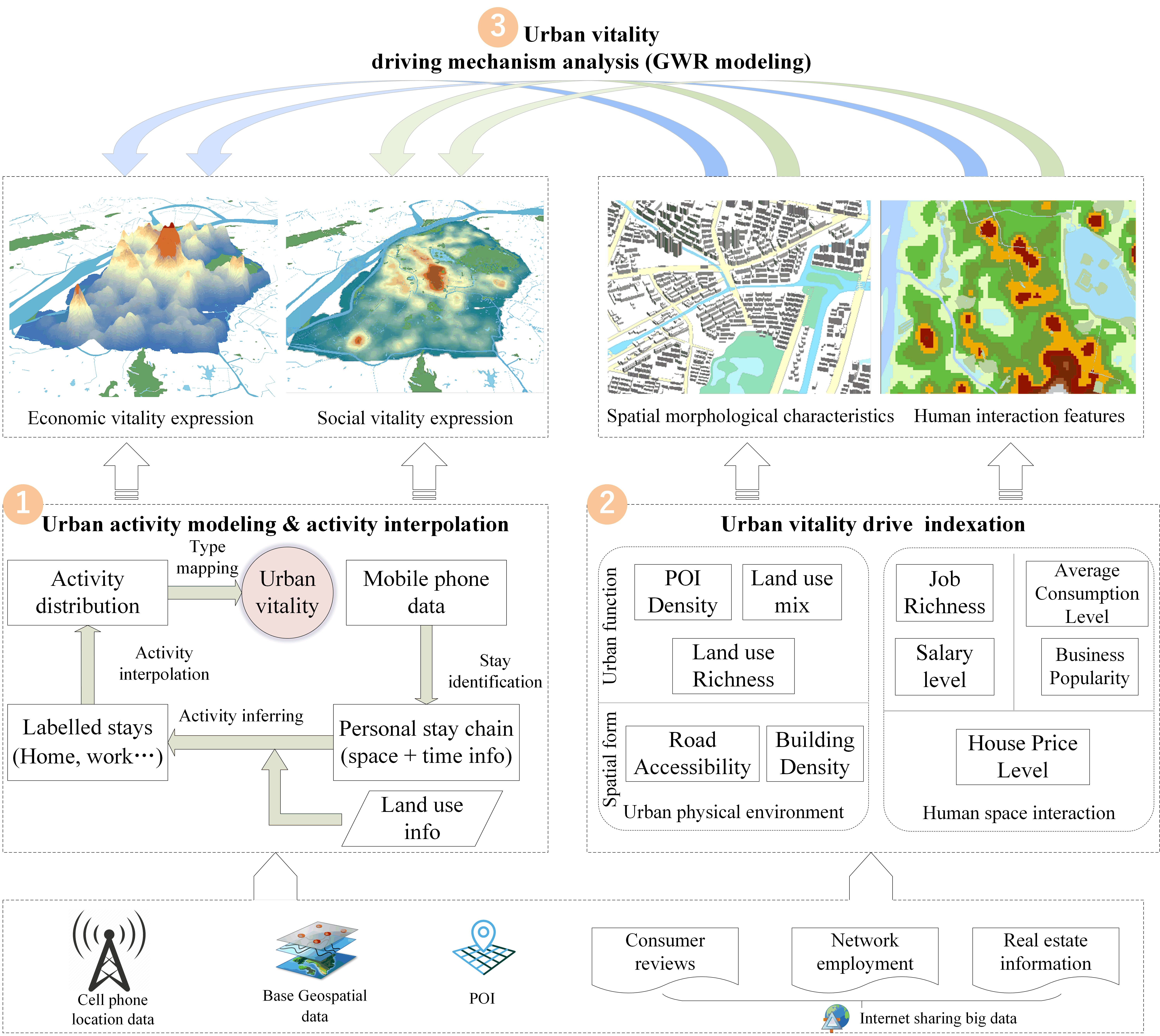
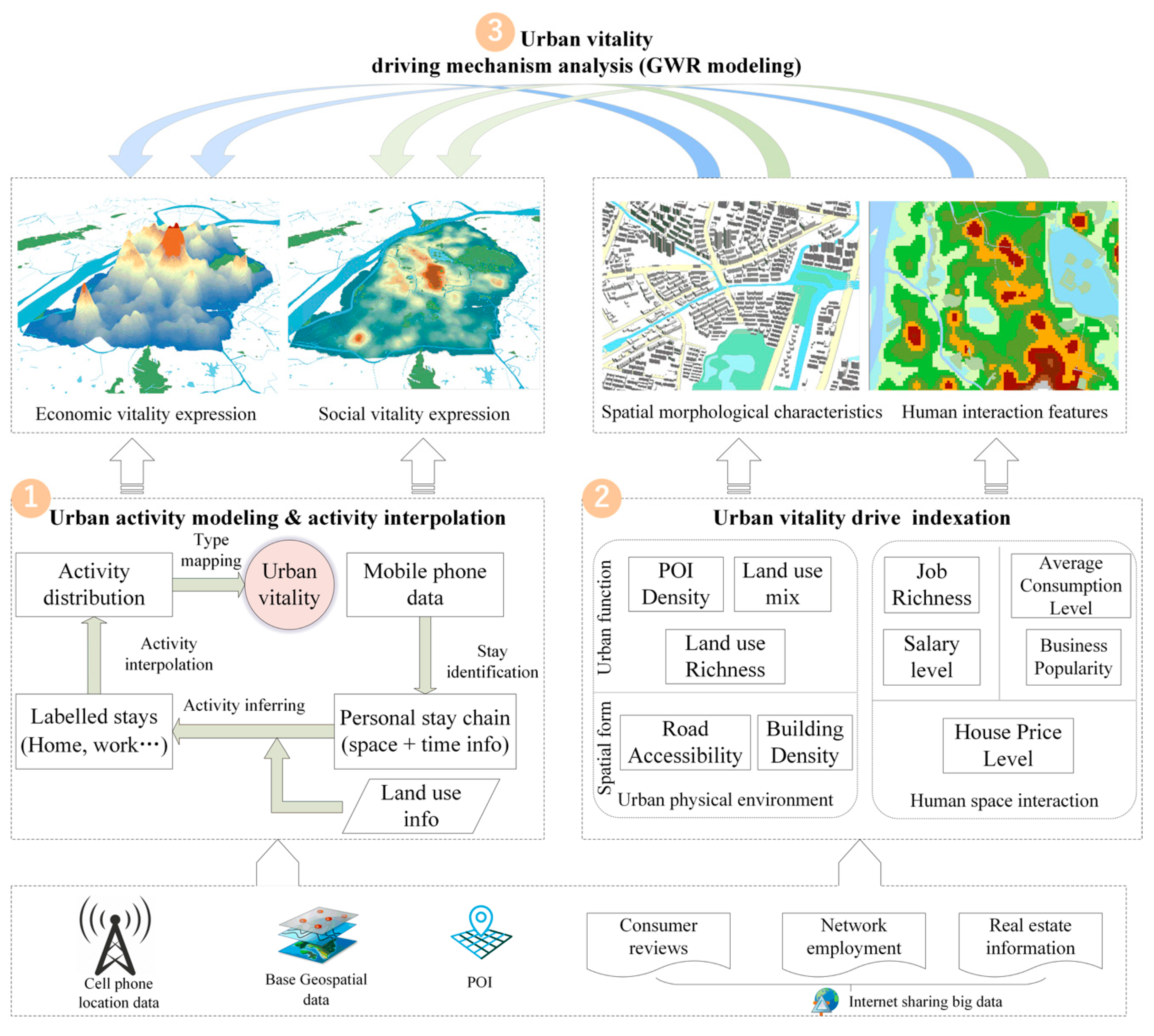
• It is a new framework for urban vitality analysis from connotation deconstruction, with explicit expression to drive mechanism exploration. Based on the modeling of human activities, this framework constructs the connotation of urban vitality and its spatial performance into economic and social aspects and realizes the mapping from human activity types to urban vitality. It is more complete and more accurate than the traditional urban vitality analysis based on population density and part of the population.
• The proposed framework makes full use of multi-source big data, and it provides a multi-dimensional drive indicator analysis method for urban vitality. Considering the shaping effect of cyberspace and social space on urban vitality, it can explore the inner driving mechanism of urban vitality from the perspective of the combination of urban physical environmental value and spatial value defined by human–land interaction.

Our frame enriches the theoretical connotation, quantitative technology, and evaluation dimension of urban vitality, and reveals the methodology of creating urban vitality from a multi-dimensional perspective. It provides certain enlightenment on how to improve urban vitality and promote coordinated and sustainable development of cities. As the process of economic globalization and urbanization continues to accelerate around the world, the global gravity center of human dynamics is constantly shifting. According to the globalization research of recent decades [32,33], the global centers of gravity are moving to East Asia (especially China), as expressed by GDP, CO₂ emissions, population, and urban population. Therefore, the research on urbanization and its countermeasures needs more examples from China. This paper takes the central metropolitan area of Nanjing, China, as the case area to verify the feasibility of this framework. Based on the exploration of the driving mechanism, we summarize the strategies for promoting urban vitality in both the economic and societal aspects.

The remainder of this paper is organized as follows. The following section describes the conceptual framework of the urban vitality quantitative evaluation, data requirements and methodology, the case study area, and experimental configuration used in the evaluation framework. The subsequent sections introduce the experimental results of the case study area, followed by the discussion and conclusions.

2. Conceptual Framework

The spatial gathering of human activities is a direct manifestation of urban vitality, and this aggregation has significant differences in spatial distribution and composition of activity categories [34,35]. According to the nature of human activity, this study divides urban vitality into two aspects: social vitality and economic vitality. The economic vitality is characterized by the spatial behavioral activities related to human production and consumption, representing the productivity and creativity of various urban spaces. It is an essential guarantee for improving the life quality of citizens [36] and making a vita-city. Social vitality is used to reflect the characteristics of people’s social behavior, including living at home, entertainment, education, and cultural activities. It demonstrates the enthusiasm of citizens to participate in urban social life, the livability of urban space, and the soft power of urban development. We regard social vitality as a necessary condition for the good and sustainable development of cities. According to the above thoughts, this paper proposes a general analysis and evaluation framework (Figure 1) for urban vitality based on activity type identification and multi-source big data fusion.

As shown in the bottom of Figure 1, three types of big data, which include mobile phone location data, geospatial big data, and internet sharing data, are used as the data source for human activity modeling and driving factor evaluating. Three core steps constitute the entire process of urban vitality measurement and evaluation, as numbered with yellow labels.

Part 1 (yellow label 1) shows the urban vitality measurement (estimation) method. It builds the individual’s movement process using mobile phone data, and it also constructs a probabilistic inference model to identify the human activity types and map them into two aspects, namely economic vitality and social vitality. Then we can analyze their specific spatial characteristics. The human movement modeling and activity type identification method will be introduced in Section 3.2.1.1, and the vitality mapping method will be described in Section 3.2.1.2.

Part 2 shows the urban vitality driving factors design in this framework. We design ten indicators to separately estimate the urban spatial attraction from two dimensions of physical and social environments. The physical dimension includes five indicators of urban physical environment evaluation. POI density (PD), land use richness (LR), and land use mix (LM) are selected to perform the urban functional feature, which is considered to be closely related to urban vitality [1,37]. Building density (BD) and road accessibility (RA) are used to assess the spatial form characteristics. Related theories suggest that a sufficient concentration of buildings and small block sizes attract more people to participate in social interaction [12,37].

The social dimension that reflects human–land interaction features is a new perspective proposed by our framework. Especially in the Information Age, when mobile Internet and LBS technology are prevalent, the relevance of ternary spaces (physical, social, and information space) becomes increasingly great. So, the behavior choice of human activities is often guided by network information [38,39]. We formulate evaluation indicators to analyze people’s interaction between social space and cyberspace on urban vitality. This framework chooses quantitative evaluation from three aspects: the human ability to obtain and create wealth adopting the indicators of salary level (SL) and job richness (JR), urban social life spending capacity adopting the indicators of the house price level (HPL), and average price level (ACL), and satisfaction with urban life services adopting the indicator of business popularity (BP). The quantitative calculation method of the above indicators will be detailed in Section 3.2.2.

Spatial regression analysis measures the degree of influence of changes in one or more variables (explanatory variables) on changes in another variable (dependent variable) by constructing regression equations between attributes of spatial objects. We use spatial regression analysis technology to analyze the correlation between the urban vitality spatial distribution and characteristics of driving factors, as shown in part 3. To make the independent variable and the dependent variable of spatial regression analysis comparable, we construct a regular uniform grid as the spatial unit for the above quantitative assessment. The GWR (Geographically Weighted Regression) modeling method will be described in Section 3.2.3.

3. Materials and Methods

3.1. Data

According to our framework, multi-source data fusion is the technical foundation of this paper. Human activity data, geospatial big data, and internet contributing big data are fused by urban spatial units. They are used to mine the characteristics of human activities, physical construction, and human–land interaction in urban space. The composition, usage, source, and contents of these data are shown in

Table 1. The input datasets are used in this framework.

Item	Usage	Contents	Source
Mobile phone data (also called “Call Detail Records”)	Human activity type inference and urban vitality measurement	User location with timestamp when they make or receive calls, send or receive text messages, switch base stations, mobile Internet, and periodic reporting in standby (usually report every half an hour)	Mobile phone communications operator
Geospatial big data	Urban vitality driving indicators estimation	Urban road network, buildings footprint with height, and fine-grained POI data	Navigation map suppliers
Internet contributing big data		1) housing price data (including community name and its average price), 2) enterprise recruitment information (including company name, job title, remuneration, and work address), and 3) the merchant review data (average consumption and reviews of each merchant); merchant types include but are not limited to restaurants, supermarkets, digital stores, etc.	The various life service website
Base station signal coverage zone	Basic supporting data	A buffer of a specified radius is created for each cell phone base station according to base station spatial distribution density, which is used to represent the user’s most likely position	Create buffer and fishnet manually
Basic statistical unit		A suitable size regular grid for quantitative measure spatial characteristics of urban vitality

.

3.2. Methodology

3.2.1. Human Activity Recognition and Urban Vitality Measurement

3.2.1.1. Personal Stay Chain and Relational Activity Recognition Model Construction

The data of human space–time activity are a basis for user activity identification. So, we need to convert the original mobile phone signaling records into individual daily activity chain data. For cellular positioning data, the speed threshold method has proved to be an effective stay recognition method that can reduce the spatiotemporal error [29,40]. Notably, the recursive look-ahead filter achieved the best performance compared to the recursive naïve filter and Kalman filter [41]. Aiming at the characteristics of spatial ambiguity and temporal sparseness of cell phone positioning data, we use the recursive look-ahead filter method to identify stays and build individual daily activity stay chains. Here are the steps:

• Data re-organization. Based on the IMSI (unique user id), the original signaling inventory data are refactored into a sequence of discrete space-time points of user daily activity in time order.
• Stay chain identification. Depending on the time, multiple consecutive records at the same location are merged into a stay point containing arrival and departure times to form a stop chain, denoted as $L$. To provide a sufficient inference basis for activity type identification, we remove the user’s single stay for less than a specified time threshold ${\Delta }_t$ from the stay chain.
• Abnormal filtering. The moving speed $v\left(i\right)$ is calculated based on the distance between $L\left(i\right)$ and $L(i-1)$ and the difference in arrival time. If $vi$ exceeds the normal linear movement speed of human activity $v_{normal}$, the distance between $L\left(i\right)$ and $L(i+1)$ is compared with the distance between $L\left(i\right)$ and $L(i-1)$. The filter removes the activity record further away from $L(i+1)$ of the activity chain.

Existing studies have shown that the type of human activity is usually closely related to the characteristics of the type of destination land use [29]. However, it is impractical to traverse the combination of all land-use features and user activity types, and features such as activity time can also influence activity type. Liao, Fox, and Kautz [42] proposed a supervised activity recognition general framework that extends Relational Markov Networks (RMNs) [43]. Their framework comprehensively considers four aspects of learning and inference activity types, namely time, space, the active transfer relationship such as “home” activity which follows “working” activity, and global constraints such as the number of homes or workplaces. On this basis, Widhalm et al. [44] extended the relational schema and proposed the expectation-maximization (EM)-based learning method, which successfully achieved unsupervised activity type inference based on mobile phone activity trajectory. This study implements the non-directional graph model, which identifies the user activity type by estimating the joint posterior probability $P_r\left(l,a|P,t,\delta ,i\right)$ of activity type and land use. $\left\{P,t,\delta ,i\right\}$ of $P_r$ represent the land-use share, activity start time, dwell time, and the number of stay chain locations, respectively, which constitute the observation variables of the relational clique template. $l$ and $a$ represent land use and activity types, respectively. They are the marker variables for the relational clique template.

Here, we instantiate four clique templates composed of an activity type distribution clique, land use type, activity type clique, time and activity type clique, and an indicator that the activity is performed at only one unique location (such as “Home”). Each clique’s potential function represents the frequency of random variable occurrences to meet its conditions, and all cliques constitute an expanded Markov network $G$. Based on the above definition, the joint probability distribution $\left(l,a\right)$ can be written as:

$$\begin{array}{cc}\mathsf{\Phi }=P_r\left(l,a|P,t,\delta ,i\right)\hfill & \\ & \propto \left[{\displaystyle {\displaystyle \prod }_{c\in C_1\left(G\right)}}{\varphi }_1\left(a_c\right)\right]\times \left[{\displaystyle {\displaystyle \prod }_{c\in C_2\left(G\right)}}{\varphi }_2\left(l_c,a_c,p_{l,c}\right)\right]\times \left[{\displaystyle {\displaystyle \prod }_{c\in C_3\left(G\right)}}{\varphi }_3\left(a_c,t_c,{\delta }_c\right)\right]\hfill \\ & \times \left[{\displaystyle {\displaystyle \prod }_{c\in C_4\left(G\right)}}{\varphi }_4\left(a_c,r_c\right)\right],\hfill \end{array}$$

(1)

where ${\varphi }_1,\cdots ,{\varphi }_4$ represent the potential function of the four clique templates. ${\varphi }_1$ is the probability distribution of each activity type, ${\varphi }_2$ represents the probability of land use ratio $p_l$ of the mobile phone station coverage zone, and activity type $a$ concerns the probability of land use type. ${\varphi }_3$ indicates the probability between arrival time, length of stay, and type of activity. ${\varphi }_4$ is a global constraint on a specific activity (e.g., a working position is highly likely to be visited once in a day, while home tends to be visited two times).

Based on the above potential function, the relationship Markov model is trained by the EM algorithm. When the distribution $\mathsf{\Phi }$ is converged, the resulting probability distribution will be used as an input to mark the most likely activity type for each user’s stay. Combined with the practical experience of related research [42,44] and the characteristics of land use type data in this study area, this research will use this activity inference method to label the following seven activity types: “Shopping”, “Catering”, “Working”, “Education and Culture”, “Home”, “Leisure or travel” and “Other”.

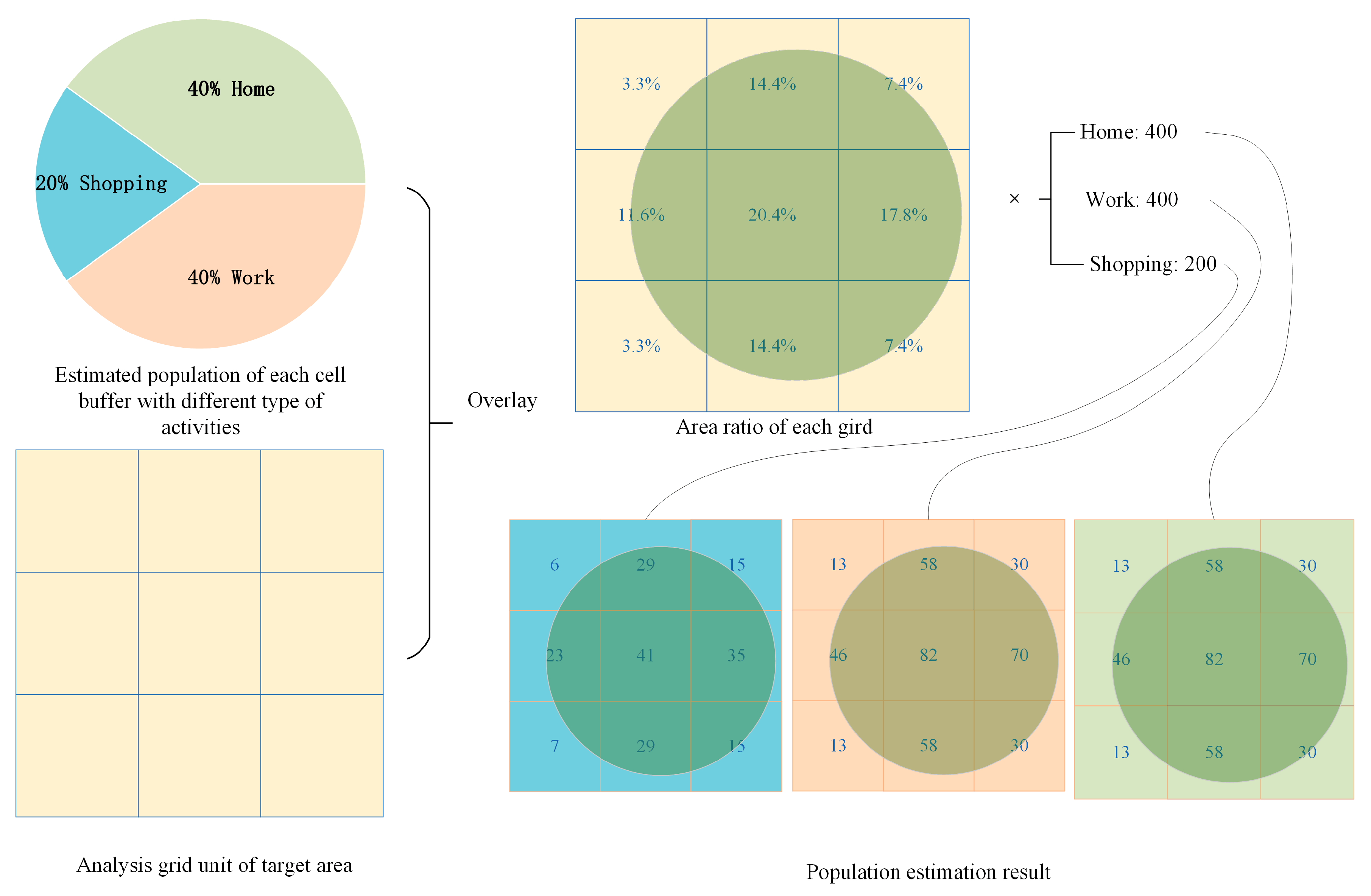
3.2.1.2. Spatial Interpolation Method for Estimating Urban Vitality Distribution

In this paper, based on the speculation of mobile phone user activity types, the spatially explicit characteristics of urban vitality are extracted by the following two steps:

We first estimate the spatial distribution of urban human activities. Currently, the two common types of method used in population distribution estimation are spatial interpolation methods and statistical model methods [45]. Among them, areal interpolation is used to solve the problem of statistical unit inconsistency. This method converts the spatial unit of the census into the actual analysis spatial unit, i.e., the conversion from the source area to the target area [46]. The activity recognition result of the stay point obtained earlier is considered to be the frequency statistics of various activities within a particular buffer zone of the user’s stay position. However, the statistical unit of human activity distribution is a regular grid unit. We design an area weight interpolation method to convert the user activity frequency of the stay points into the activity intensity distribution of a corresponding grid statistical unit, as shown in Figure 2. The activity intensity is calculated as the ratio of the frequency of various activities to the area of the spatial grid unit.

Next, the spatial distribution of urban vitality is determined by defining the mapping relationship between activity type and vitality. Here we describe the mapping relationship between activity type and vitality based on the definition of economic vitality and social vitality and the nature of human activity type based on our urban vitality analysis framework. The results of the mapping relationship are shown in

Table 2. Mapping relations between activity types and urban vitality aspects.

Activity Type	Activity Superclass	Vitality Aspect
Shopping (S)	Consumption	Economic vitality
Catering (C)
Working(W)	Production
Education and Culture (E)	Social life	Social vitality
Home(H)
Leisure or travel(L)
Other(O)

. Economic vitality is expressed through human economic activities, and people’s daily economic activities are characterized by consumer buying activities and productive activities as producers, and they have direct benefits for urban economic growth and development [47]. Specifically, the activity modeling identified shopping and catering activities are summed up as consumption activities, and the working activity corresponds to the production activity—they together constitute the economic vitality of the city. Building a livable urban environment and open public spaces, promoting people’s social interaction, and integrating them into urban life is an essential aspect of urban vitality [1,10]. Participation in recreational activities, cultural and educational activities, and family life reflects urban social life, so they are mapped to social vitality. Additionally, “Other” activity is also integrated into social vitality. It indicates other types of activities, such as people walking on the street.

3.2.2. Quantification Calculation of Vitality Impact Factors

After collecting and processing GIS spatial big data and the internet contributing big data, this paper constructs and quantifies ten potential driving indicators of urban vitality. These indicators evaluate the two-dimensional ground value of urban ground physical built environment and human–land interaction characteristics. The meaning and calculation of the indicators are shown in

Table 3. Quantification calculation method for urban vitality impact factors designed in our framework.

Dimension	Indicator	Equation	Number	Data Source	Description
Physical built environment (urban function dimension)	Land use richness (LR)	$LR={{\displaystyle \sum }}_{i=1}^n{p}_i^0$	(2)	POI	Refer to Yue et al.’s work [13]
	Service facility density (PD)	$PD=\frac{{{\displaystyle \sum }}_{i=1}^{n}Nu{m}_i}{A}$	(3)
	Land use mix (LM)	$LM=-{\displaystyle {\displaystyle \sum }_{i=1}^n}{p}_i\ast ln\left(p_i\right)$	(4)
Physical built environment (urban design dimension)	Building density (BD)	$BD=\frac{{{\displaystyle \sum }}_{i=1}^n\left(h_i/H\right)\ast a_i}{A}$	(5)	Building profile	We design this equation that takes into account floor height and footprint
	Traffic access (RA)	$RA=\frac{{{\displaystyle \sum }}_{i=1}^{n}j}{A}$	(6)	Road network	RA is evaluated by extracting and calculating the number of road intersections in each region
Human-land interaction dimension	Business popularity (BP)	$BP=I\left(reviews\right),$ $I\left(v\right)=\frac{K\left(v,radius,pts\right)}{A_i}$	(7)	Merchants info from life service website	It is reflected by the number of merchant reviews
	Average consumption level (APL)	$ACL=I\left(price\right)$	(8)		Merchants’ average consumer prices are used as input data
	Salary level (SL)	$SL=I\left(salary\right),$ $jo{b}_e={{\displaystyle \sum }}_{i=1}^n{j}_i^0\ast nu{m}_i$	(9)	Corporate recruitment website	The average salary of each company is used as input
	Job richness (JR)	$JR=I\left(jobs\right),$ $s_e=\frac{{{\displaystyle \sum }}_{i=1}^n{j}_i-\max \left(j\right)-\min \left(j\right)}{n-2}$	(10)		The number of jobs provided in each company is selected to reflect job richness
	House price level (HPL)	$HPL=I\left(hp\right)$	(11)	Real estate information website	Each residential community’s average house price is used as input

.

In the first three formulas, $p_i$ is the proportion of the i-th POI type for the total POI records, $n$ is the total number of the POI type, $Nu{m}_i$ is the number of each POI type, and $A$ is the area of each patch (spatial analysis unit). The LM indicator is used to reflect the orderliness of land use type and its quantity—the higher the value, the more ordered the land type is, while on the contrary, a lower value means disorder and randomness. $h_i$ and $a_i$ in Equation (4) represent the floor height and floor area of the $i$-th building. $H$ indicates the highest floor height in the study area, and $A$ indicates the area of a statistical unit.

For human–land interaction dimension indicators (the last five indicators in Table 3), the Ordinary Kriging (OK) interpolation method is used to estimate the spatial distribution of analysis indicators. Sample points collected from related websites are used to estimate the spatial distribution of analysis indicators used as the input data. $I\left(v\right)$ is a general equation design for spatial estimation as shown in Equation (7), where $K$ is the OK interpolation method, $radius$ is the search radius, $pts$ is a specified number of input sampling points, and $A_i$ is the area of $i$-th analysis unit. BP and APL reflect the consumption heat and consumption level in various urban regions and reflect the quality of life services. The level of the SL indicator reflects each region’s economic creativity, and each company’s average salary is estimated as removing the remuneration of the highest and lowest positions and calculating the average value of the remaining remuneration range data, see the equation $jo{b}_e$ in (9). The JR indicator reflects the demand and attractiveness of talent in each region, and it is represented by the number of jobs offered by each enterprise (see Equation (10)). In Equations (9) and (10), $j_i$ is the average salary for the $i$-th position of the $e$ enterprise, $nu{m}_i$ is the number of recruits for this position, $n$ is all positions of the $e$ enterprise, and $j$ represents the average salary set of $e$ enterprise. The HPL indicator shows the fundamental value of urban space; the level of housing prices not only correlates with the location but also reflects the consumption capacity of a region.

3.2.3. Spatial Regression Analysis of Urban Vitality

Regression modeling is a statistical data analysis technique. It provides us with an effective means for understanding the relationship between independent variables and explanatory variables. Multiple regression analysis techniques have been successfully applied in the research of physical phenomenon simulation [48], population growth and spatial location factors modeling [49,50,51], economic fluctuation trend fitting and prediction [52], and tourism research [53,54]. The spatial regression model has been successfully applied to the study of the correlation between urban vitality and land-use characteristics [11,19]. However, the ordinary least squares (OLS) model is suitable for global feature analysis, and it does not consider spatial non-stationarity. If the data are spatially dependent and ignored, it will often produce misleading results [55]. Since the spatial distribution characteristics of different vitality driving factors always show significant differences, the impact of various factors on urban vitality will also be different in multiple regions. To reveal the driving mode of urban vitality of urban built environment and interaction between human and urban space, we adopt the local linear regression model, the GWR model, which takes into account the spatial self-correlation parameters as the modeling method. The mathematical form of the GWR model is:

$$y_i={\beta }_0\left(u_i,v_i\right)+{\displaystyle \sum }_{k=1}^p{\beta }_k\left(u_i,v_i\right)x_{ik}+{\epsilon }_i,$$

(12)

where the $y$ is a dependent variable observation, and $\left(u_i,v_i\right)$ is the coordinate of the observation point $i$. ${\beta }_0$ is the regression coefficient of the i-point, indicating the degree to which the argument affects dependent variables. $p$ is the number of independent variables, $x_{ik}$ represents the value of the $k$-th independent variable of position $i$, and ${\beta }_k$ is the $k$-th regression coefficient of the $i$-th point. ${\epsilon }_i$ represents a random error, which is a normal distribution function with a constant variance.

Here, the driving indicator constructed in Section 3.2.2 is taken as the explanatory variable $x_i$, and the urban economic vitality and social vitality intensity estimated in Section 3.2.1.2 are used as the dependent variable $y_i$. Furthermore, this paper will adopt the idea of exploratory regression analysis, and we try to construct the GWR model of urban economic vitality and social vitality using different combinations of explanatory variables. After the successful construction of the model, diagnostic indicators such as residual squares, AICc, R2, and adjusted R2 will be output to reflect the performance of the model. The lower the value of AICc and the closer R2 is to 1, the better the fit of the result. Then, we obtain the optimal analysis model according to the diagnostic coefficient. Finally, the optimal model will answer questions about which factors contribute to the urban economic vitality and social vitality and how they work.

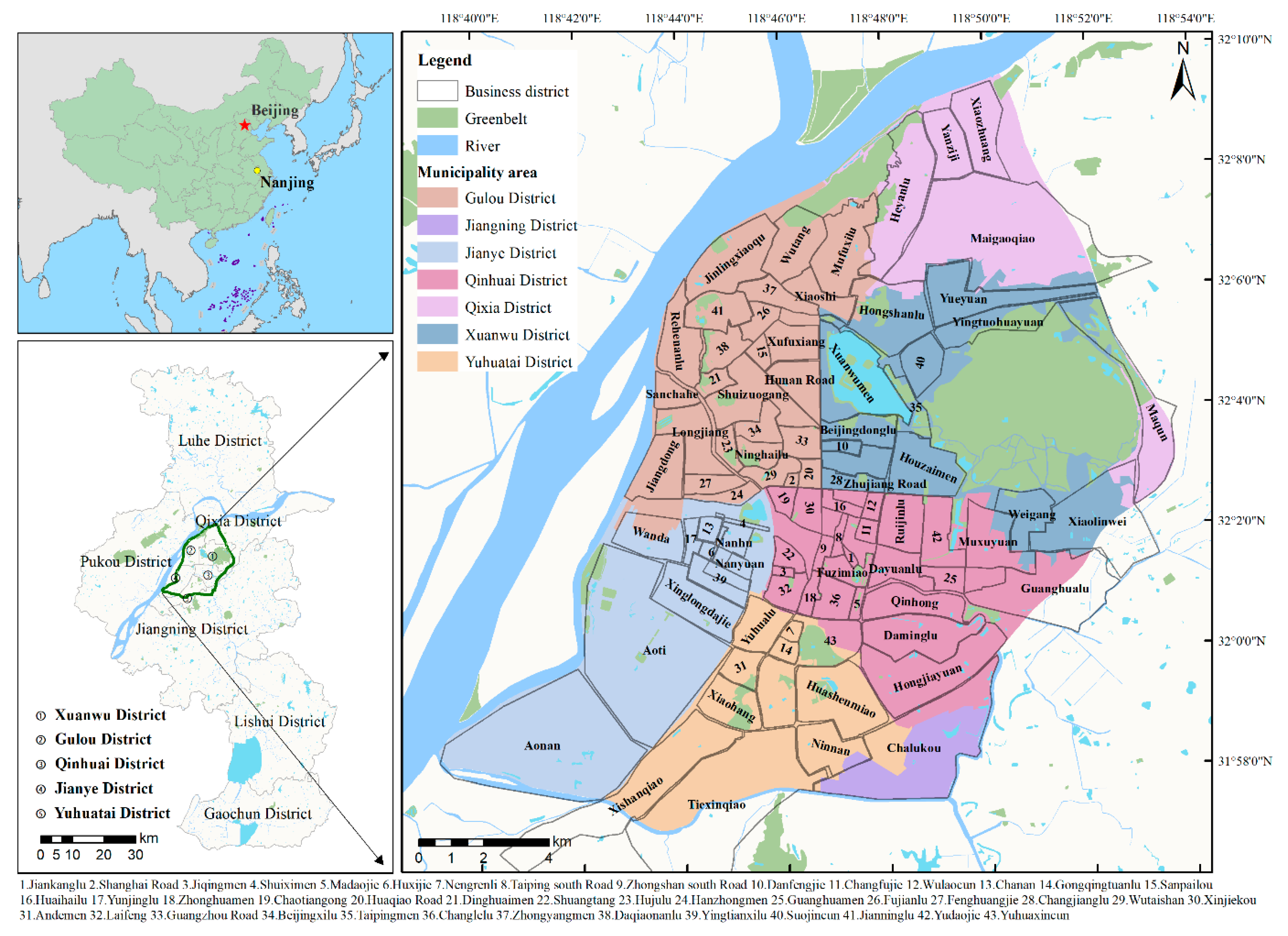
4. Case study Area and Experimental Design

4.1. Case Study Area and Experimental Data

Nanjing is a megacity in the Yangtze River Delta City Cluster, which is the most economical vita resource allocation center of China. The size of Nanjing is second only to Shanghai in this City Cluster. We select the main urban area of Nanjing (according to Nanjing 2011-2020 master plan) as our case study area. This area is located in an urban area with Xinjiekou CBD (Central Business District) as the core. It is a highly urbanized area where population and urban functions gather. Therefore, the embodiment of urban vitality and the formation mechanism of urbanization can be fully reflected here. The geographical location, administrative divisions, and business district distribution of the study area are shown in Figure 3. According to the urban vitality evaluation framework proposed in Section 2, geospatial big data, mobile phone data, and the Internet contributing big data are obtained as research data. Their specific descriptions are detailed in

Table 4. A detailed description of the data source used in our empirical research.

Item	Source	Quantity	Time
Mobile phone data	A Chinese communications operator (China Telecommunications Corporation)	5,553,743 anonymous mobile phone users and 268,990,535 original records	April 1, 2019
Building profiles	China’s largest map service platform AMAP (https://www.ditu.amap.com)	121,193	April 2020
Road network		national, provincial, and county roads
POI		53,487
Business data	Dianping website, China’s most extensive used lifestyle service review site, http://www.dianping.com	18,719
House price	Fangtianxia website, China’s leading real estate information website, https://nanjing.fang.com	3485
Recruitment info	51job website, China’s the largest job publishing website (https://www.51job.com/)	13,250

Note: For user activity type inference needs, the original 20 categories of POI are merged into 13 categories. They are catering services, shopping services, life services, sports and recreation services, medical services, accommodation services, tourist attractions, residences, governmental organizations, science/culture and education services, transportation services, finance and insurance services, and enterprises.

.

4.2. Experimental Parameter Settings

To facilitate the spatial characteristic expression and correlation analysis of urban vitality, we divide the study area into 200*200 m grids as spatial analysis units by considering the spatial error of mobile phone location data. $v_{normal}$ was set to 5.43 km/h according to a pedestrian average walking speed and the time threshold of a single stay ${\Delta }_t$ = 15 min. Since individual stops may be spread throughout the city, the activity type label of the user’s stay chain is expanded to the entire city of Nanjing. Simultaneously, considering the non-uniform distribution of base stations in space, this paper creates 250 and 500 m buffer zones for base stations in urban areas and outside urban areas. Then, it calculates the proportion of POI types in each buffer zone as the probability coefficient $p_l$. The spatial interpolation of the human–land interaction indicator uses the Gaussian Semivariogram, with the search point of 10 and the maximum search radius of 1km.

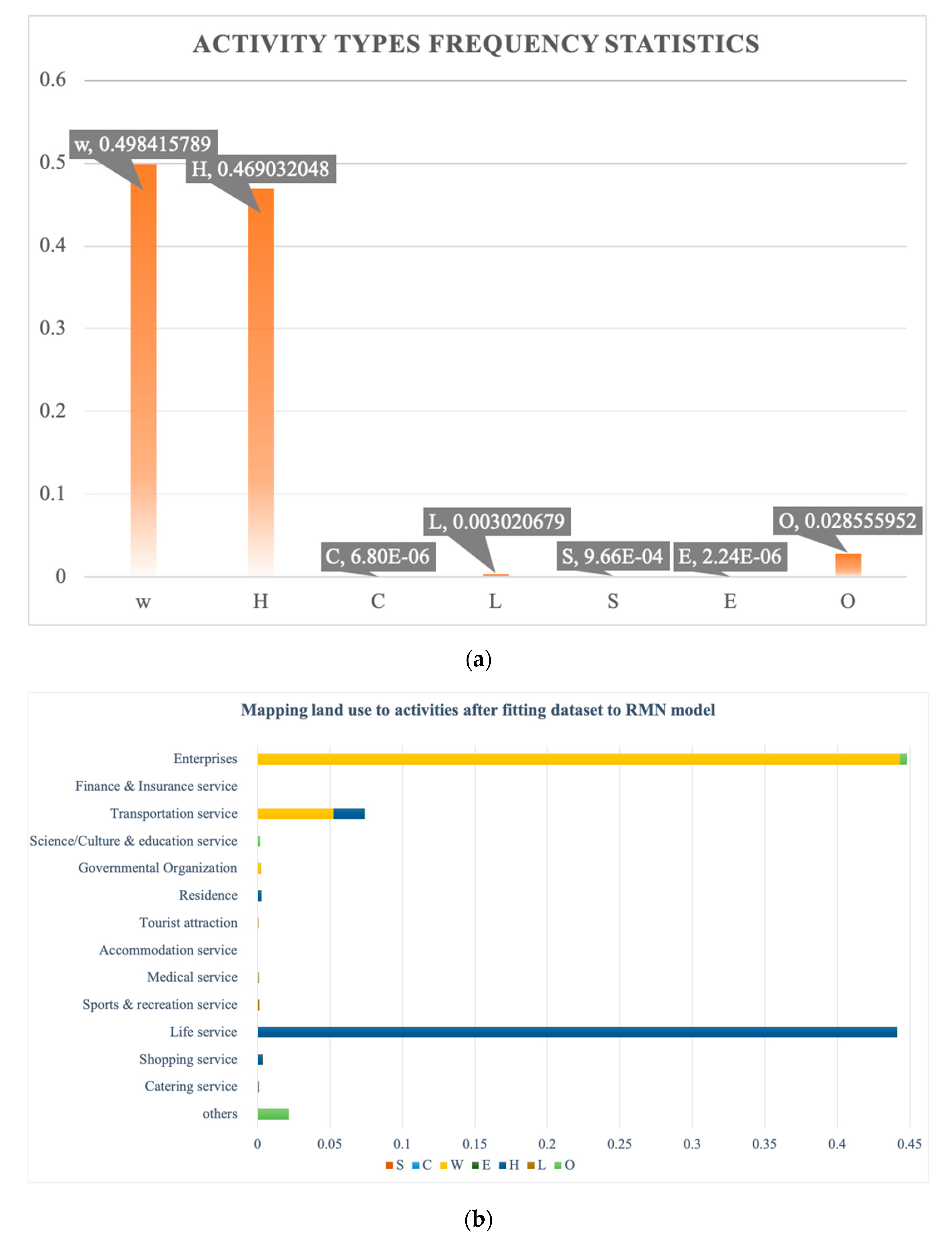
4.3. Activity Types Inference Probability Model Training

Before using the activity recognition model to speculate on the type of activity that the user stays in, we need to initialize the prior probability for the model. ${\varphi }_1$ is initialized as a uniform distribution. Prior knowledge is used to set the correlation between land use and activity type to initialize ${\varphi }_2$. According to the strength of the correlation, it is divided into three weight levels of 1-10-1000—the higher the level, the stronger the correlation (e.g., the activity type “Home” is most likely to correspond to the land use type “Residence”), and normalize them to a ratio of 1, so that the sum of the probabilities of all activity types is 1. ${\varphi }_3$ consists of two parts: start time $w_t$ and length of stay $w_s$ mapping with various activities. It is divided into three levels of 1-10-100, and a higher value indicates a greater possibility of engaging in such activities at that moment and stay. We construct a $w_t\times w_s$ matrix to initialize $p(a|t,\delta )$. ${\varphi }_4$ is used to set global limits on specific activities. If an individual’s activity has been returned, the probability that the activity type is “Home” is 1, and the probability that the activity type is outside the “Home” is 0.5.

After using the above initialization parameters and the daily activity chain of 20,000 users as a training sample, we successfully construct an activity inference model. After 36 iterations, the model is convergent. The activity types of 13,248,925 stays were finally identified, with an average number of daily stops per user of 3.63. As shown in Figure 4a, “Work” accounts for the largest share of people’s activities, followed by “Home”, and the smallest proportions of activity types are occupied by “Education” and “Catering”. The reason for this is that ordinary workday data are used as the data source, and there are fewer meals outside on weekdays; mobile phone users are mainly adult groups, the proportion of educational and cultural activities is small. In addition, Figure 4b shows the joint probability distribution between land use and activity types. It reflects the land use distribution of the study area. The land type of life services and enterprise account for a relatively high proportion, and they are mainly mapped to “Work” and “Home” activities.

5. Results

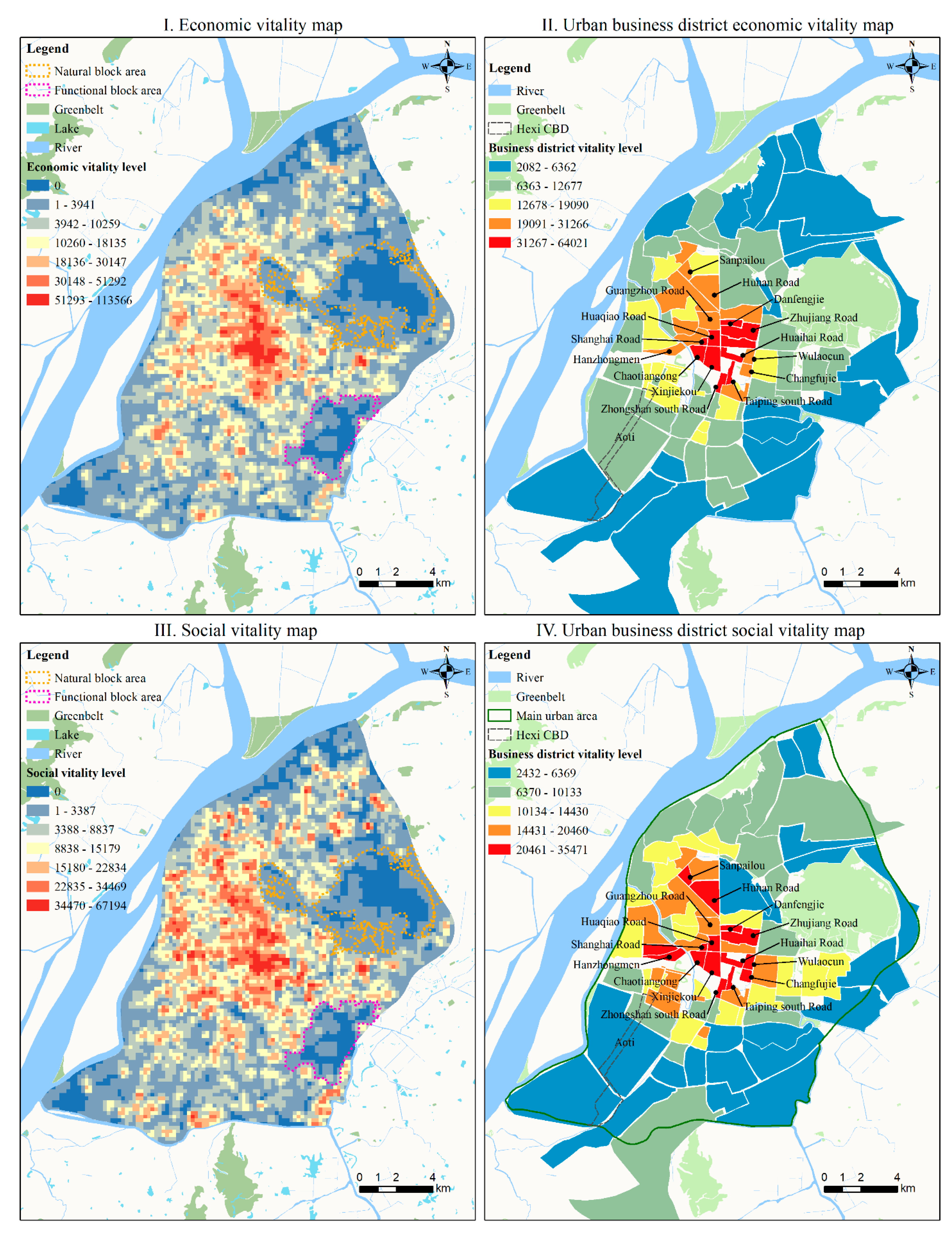
5.1. Spatially Explicit Features of Urban Vitality

Based on the activity recognition results in Section 4.3, the method of area weight interpolation is used to estimate the economic vitality intensity and social vitality intensity of each analytical unit according to the mapping relationship between activity type and urban vitality. As shown in Figure 5I,II, most of the areas with high economic vitality are concentrated in the central area. Their distribution presents a ring-type structure from inside to outside. The economic vitality of Xinjiekou CBD and its adjacent areas, such as Huaihai Road and Huaqiao Road, is the highest. It is followed by a business district like Guangzhou Road and Hunan Road. The economic vitality of the outer business areas where are filled in blue is relatively low. Although the Aoti business district covers the financial district of Hexi CBD, its overall vitality level has been reduced, affected by its broad coverage area. As seen from Figure 5III,IV, the spatial distribution of social vitality is relatively more dispersed, and the range of high-vital regions is relatively large. For example, the business district of Sanpailou and Hanzhongmen far from Xinjiekou CBD become the highest-level vitality area, while they are at the second level in terms of economic vitality. Meanwhile, the higher level of social vitality districts is more gathered in the northern region than that of the southern region. The orange dotted area in Figure 5 is a low-vitality area blocked by mountains and lakes. In contrast, the Pink Ginger dotted area is a vibrant cold zone due to the sparseness of urban function (reference POI density, Figure 6a-4).

The above results reflect that the central area dominates the urban economic development, and contributes a lot of production creativity to the city. The high-level economic vitality districts have more hotness than social vitality districts. Furthermore, social vitality distribution mainly reflects the pattern of people’s living, leisure, and recreation space.

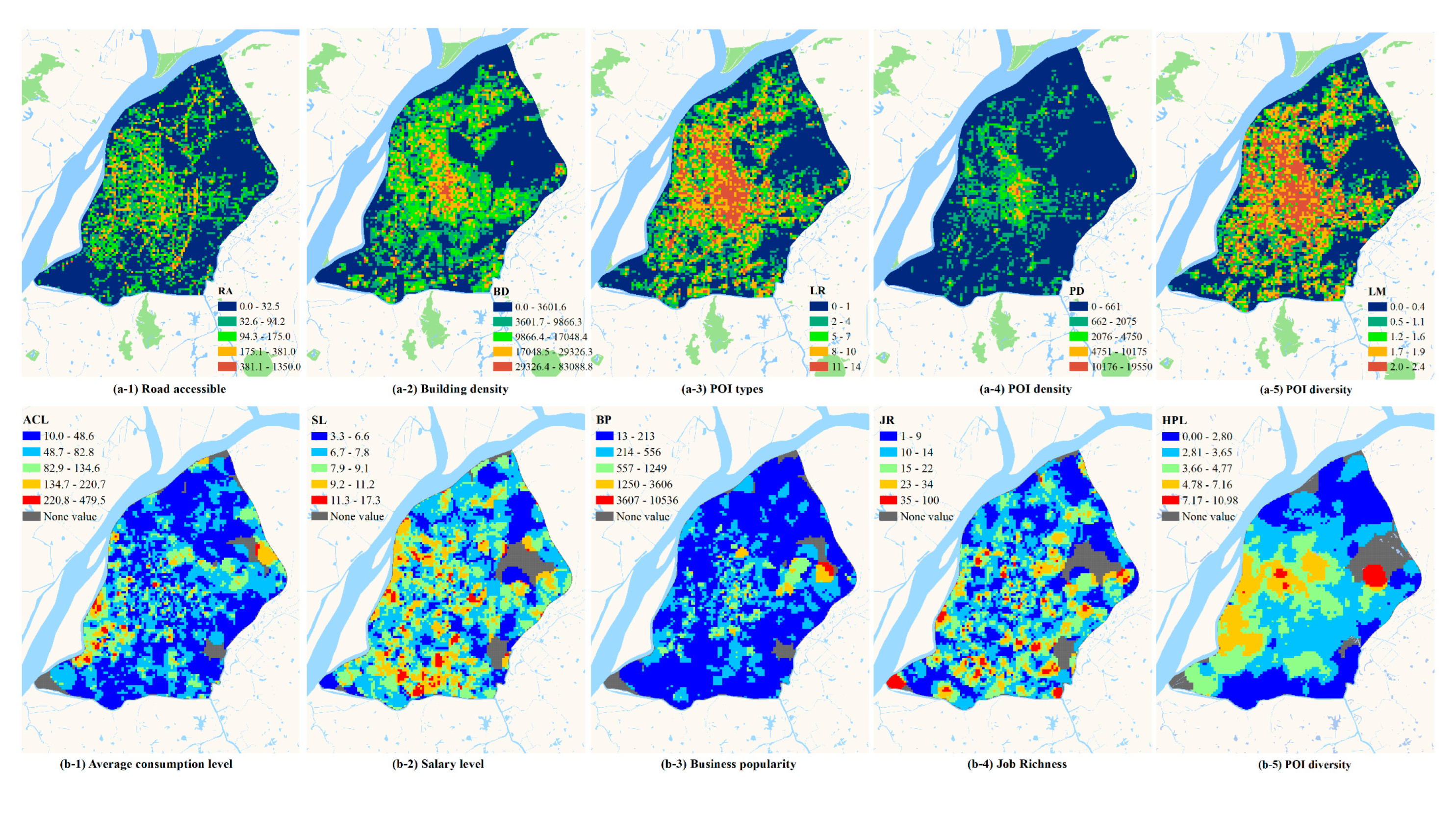
5.2. Quantitative Results of Vitality Impact Indicators

Quantitative results of physical built environmental indicators and human–land interaction indicators are shown in Figure 6. For comparison, the evaluation results are divided into five levels by the natural breaks classification method.

According to Figure 6a-1 to a-5, it is found that RA and BD are mainly concentrated in the middle numerical interval, and the traffic accessibility of large areas in the central and western regions of the study area is relatively convenient (a-1, a-2). At the same time, the spatial distribution of medium and high building density is more uniform (a-2). The spatial differentiation of PD is relatively more prominent. The central area is a high PD concentration area (a-4). In contrast, the peripheral area has a lower value, which reflects the characteristics of urban functions radiating from the center to the surrounding. The two remaining indicators (a-3, a-4), especially the middle and high LM value, cover most of the study area, indicating that the urban functional diversity is relatively complete in most areas.

In Figure 6b-1 to b-5, the high business popularity (BP) area is mainly distributed in the urban center (b-3), while the high urban consumption level (ACL) area is close to the beautiful surrounding tourist areas and Hexi financial center area (b-1). According to the distribution of SL and JR indicators (b-2, b-4), urban employment opportunities and salary treatment are often related to the industry. The wages of employees in the technology and financial industries are usually relatively high, concentrated in the central and southern regions of Figure 6b-2. Employment opportunities are related to the size of enterprises and the accumulation of industries. Large-scale group enterprises and industrial parks have a high demand for talent, attracting many population pooling, and the spatial distribution in this study area is more scattered (b-4). In contrast, the spatial continuity of urban housing prices is strong, and the high-value areas for housing prices in the study area are mainly central urban areas and Hexi areas, which are closely related to the high-quality educational resources of the central urban areas and the leading economic development in the Hexi area (b-5).

To avoid multicollinearity problems with multiple explanatory variables, this paper eliminates the possibility of redundant explanatory variables by calculating the variance factor inflations (VIF) indicator. Generally, when VIF is less than 10, there is no multicollinearity. After verification, it is found that PT and LM have a VIF greater than 10 in the linear regression diagnosis with economic vitality and social vitality. So, we remove the PT to keep VIF less than 10. In addition, the GWR modeling requires spatial autocorrelation of variables, and we use Moran’s I index [57] to test the spatial self-correlation of dependent variables before building the GWR model. After inspection, the Moran’s I values of economic vitality and social vitality are 0.85 and 0.80, respectively. This indicates that there is a spatial aggregation of similar values and different values in urban vitality intensity.

This paper takes the economic vitality intensity and social vitality intensity as the dependent variables. It uses multiple combinations of physical built environmental indicators and human–land evaluation indicators as the explanatory variable to construct the GWR model. The model construction results are detailed in

Table 5. Comparison of GWR model diagnostic indexes constructed by different indicators combinations.

Analysis Dimension	Model	BD	RA	PD	LM	SL	JR	BP	ACL	HPL	R2	Adjusted R2
Physical environment	PEM4	√	√	√	√						0.788	0.755
	PEM3*		√	√	√						0.819	0.779
	PSM4	√	√	√	√						0.715	0.671
	PSM3*		√	√	√						0.751	0.695
Human interactive	HEM4					√	√	√	√		0.586	0.572
	HEM3*						√	√	√		0.690	0.660
	HSM4					√	√	√	√		0.506	0.490
	HSM3*						√	√	√		0.595	0.557

Note: Only the same number of explanatory variables are listed here due to the construction of the best analysis model for input.

. According to the diagnostic indicators of the modeling results, the models marked with an asterisk in the table (such as PEM3* and PSM3*) have better performance than unmarked models (such as PEM4 and PSM4). So, it turns out that the more explanatory variables there are, the better the modeling effect. Appropriate variable combinations can complement each other and prompt the regression model to fit the change in the dependent variable to the greatest extent. Finally, this study constructs the driving analysis models PEM(PEM3*), HEM(HEM3*) for economic vitality, and the driving analysis models PSM(PSM3*), HSM(HSM3*) for social vitality from two dimensions: physical analysis indicators and human–land interaction indicators. The modeling results are shown in

Table 6. GWR modeling results for economic vitality and driving indicators.

Diagnostic Index		Physical Variables Based Economic Vitality GWR Model (PEM)			Human Interaction Variables Based Economic Vitality GWR Model (HEM)
Residual Squares		153,783.93			248,951.44
AICc		44,865.01			42,942.52
R2		0.8199			0.6903
Adjusted R2		0.7798			0.6609
Bandwidth		542.7			795.7
Explanatory variables coefficients
Model	Dependent variable	Explanatory variables	Min	Lower quartile	Median	Upper quartile	Max	SD
PEM	Economic vitality	RA	−0.0727	−0.0031	0.0030	0.0124	0.1495	0.0171
		PD	−0.0176	0.0012	0.0025	0.0041	0.0321	0.0032
		LM	−8.3981	0.6835	1.7479	3.1665	23.0136	2.4757
HEM	Economic vitality	JR	−0.9305	−0.1067	0.0052	0.1707	0.8641	0.2461
		BP	−0.0391	−0.0039	0.0008	0.0079	0.0691	0.0109
		ACL	−0.4178	−0.0446	−0.0132	0.0155	0.2851	0.0616

and

Table 7. GWR modeling results of social vitality and driving indicators.

Diagnostic Index		Physical Variables Based Social Vitality GWR Model (PSM)			Human Interaction Variables Based Social Vitality GWR Model (HSM)
Residual Squares		143,002.56			213,955.94
AICc		44,338.33			41,959.52
R2		0.7510			0.5954
Adjusted R2		0.6955			0.5571
Bandwidth		542.70			795.73
Explanatory variables coefficients
Model	Dependent variable	Explanatory variables	Min	Lower quartile	Median	Upper quartile	Max	SD
PSM	Social vitality	RA	−0.0906	−0.0050	0.0017	0.0093	0.1005	0.0158
		PD	−0.0110	0.0008	0.0019	0.0039	0.0197	0.0032
		LM	−7.4257	0.6300	1.8957	3.6719	18.3644	2.5013
HSM	Social vitality	JR	−0.8865	−0.0859	0.0311	0.1966	1.1197	0.2399
		BP	−0.0603	−0.0069	−0.0018	0.0027	0.0837	0.0108
		ACL	−0.2571	−0.0446	−0.0133	0.0182	0.3064	0.0650

, respectively.

6. Discussion

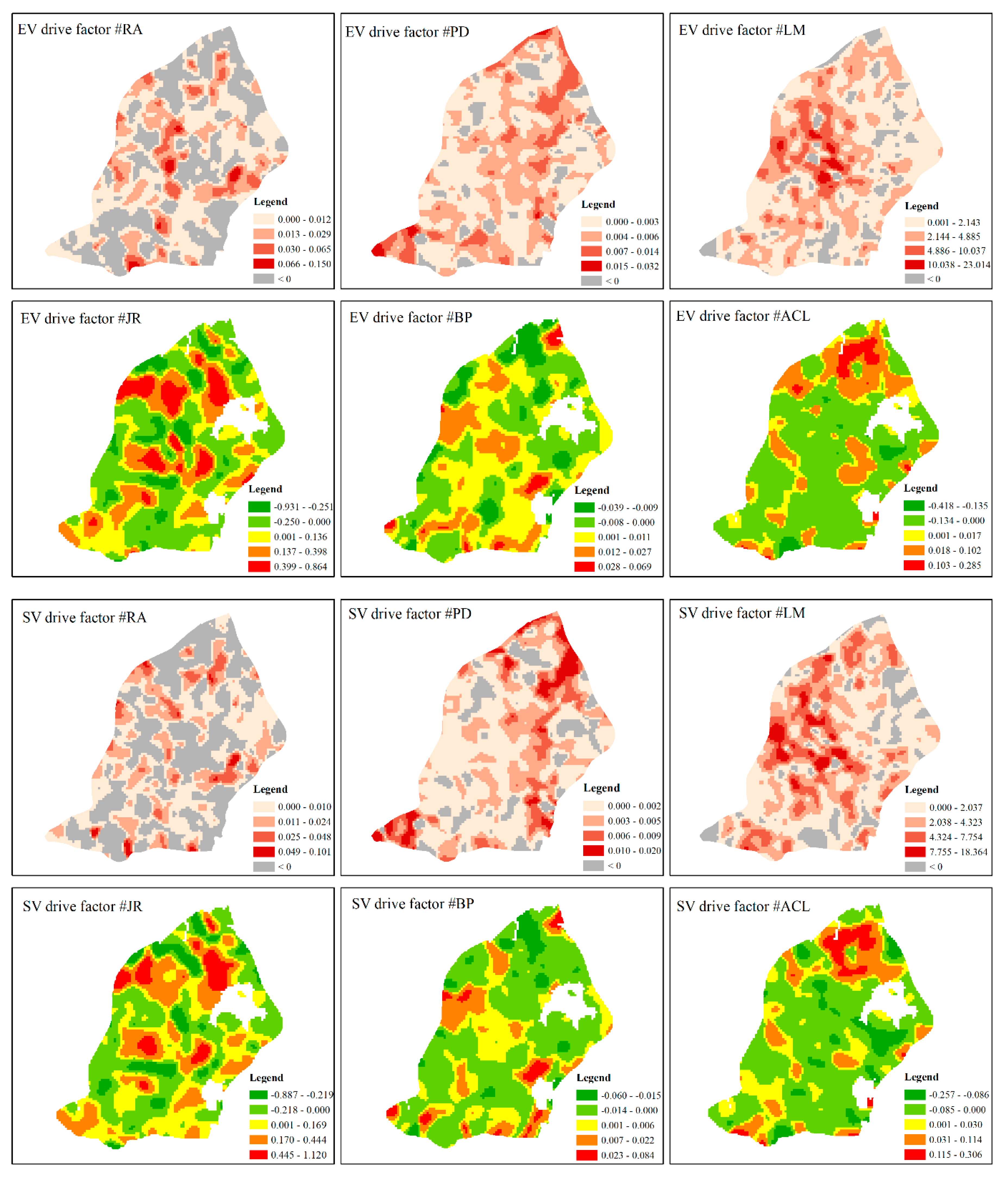
6.1. What and How Explanatory Variables Stimulate Urban Economic Vitality or Social Vitality?

The spatial distribution of each explanatory variable coefficient of the economic vitality driving model PEM, HEM, and the social vitality driving model PSM, HSM is shown in Figure 7. Combining the GWR modeling results and Figure 7, we can summarize the following conclusions.

First, the most significant variables of the physical environment influencing urban economic and social vitality are RA, PD, LM. The LM indicator has the most noticeable impact (the standard deviation of the LM coefficient is the largest, which is 2.4757 and 2.5013, respectively). In contrast, BD has no significant driving effect on urban vitality in this study area (as shown in Table 5, PEM4 and PSM4 reduce the interpretation of urban vitality after adding BD indicator). The medians of the three physical environment explanatory variable coefficients of the PEM and PSM models are all positive. This demonstrates that superior urban transportation accessibility (urban form), adequate service resource facilities, and mixed land use (urban function) are necessary conditions for stimulating urban economic and social vitality. They are an essential guarantee for forming good space quality and perfecting space function. In addition, the outstanding driving performance of the LM variable on the urban vitality proves that a complete and balanced service resource allocation is an essential manifestation of the development maturity of the regional urban function. This coincides with the research conclusions [19,58] on the physical driving factors of urban vitality. The difference between this article and Huang et al. [20] is that their research did not consider spatial non-stationarity, and they listed both BD and PD as the two most important factors driving urban vitality. However, the GWR modeling results in this paper show that BD has local multicollinearity with other driving indicators. This may be explained for urban vitality instead by other indexes such PD.

Second, the three indicators of JR, BP, and ACL have the most robust explanatory degree for modeling economic vitality and social vitality in terms of the human–land interaction dimension. In contrast, the driving effect of HPL on urban vitality is not significant. This shows that resident employment and online reviews have a considerable impact on modern urban life. Furthermore, by comparing the standard deviation of all indicators, it is found that the JR indicator has the most significant variation range in urban vitality, and BP has the smallest variation range. This shows that not only is economic vitality directly affected by abundant employment opportunities, but also people expect that their place of residence is as close as possible to areas with abundant job opportunities, thereby reducing commuting distance. Meanwhile, low consumption (median value of economic vitality ACL coefficient is less than 0), and sufficient employment opportunities are favorable conditions for activating urban economic vitality. Social vitality is more affected by online reviews (the ACL coefficient value of social vitality is higher than economic vitality), and popular life service places greatly attract people’s social lives.

Third, the impact of various indicators on urban vitality has apparent spatial heterogeneity. As we can see in the first and third row of Figure 7, RA and LM have the most noticeable impact on the economic vitality in the central area of Nanjing’s main urban area, while PD’s effects are more global. Unlike economic vitality, social vitality is weakened by the traffic advantages (RA) in the urban center area, while the impact of PD and LM is strengthened. From another aspect, as shown in the second and last row of Figure 7, JR has an overall spatial driving effect on the urban economy and social vitality. On the contrary, the ACL is more negatively correlated with urban vitality, and the BP coefficient of the corresponding region is mostly positive. Overall, good traffic conditions and reasonable rents not only attract a large number of companies and businesses to settle in, creating more job opportunities, but also increases the convenience and livability of life. Meanwhile, people wish for low-consumption and high-reputation services most of the time.

6.2. How to Increase Urban Economic Vitality and Social Vitality?

The regions with the highest levels of economic and social vitality intensity are extracted as high vitality areas, respectively. The statistical distribution of each driving indicator in the high vitality areas is shown in Figure 8. Based on analyzing the statistical characteristics of the driving indicators in these areas, the following conclusions are summarized about how to effectively improve urban economic and social vitality.

(1) Economic vitality improvement strategies. From the perspective of physical space, urban high economic vitality areas are more concentrated than social vitality. High economic vitality has a strong positive correlation with road density and land use mix; the higher the land mix, the stronger the vitality, and the road density can be maintained within an appropriate range (94-380 nodes/km² in our study area). Economic vitality and POI density are linearly related in space and value. The closer to the central area, the higher the PD density and the more influential the economic vitality. From the perspective of human–land interaction, the positive correlation between urban economic vitality, employment opportunities (JR), and business enthusiasm (BP) is relatively significant. The positive association between BP and ACL is more influential in the central urban area than in the peripheral areas. It shows that great employment opportunities and low consumption are directly related to the performance of the urban economic vitality, and the central urban area needs more job opportunities and high-quality business services (to attract more consumer groups). Despite the reduced service level in the surrounding areas, lower consumption levels are needed as alternative conditions.

(2) Social vitality promotion strategies. The area with high social vitality is relatively scattered, and the spatial heterogeneity is relatively small. That is, to improve urban social vitality, more balanced space quality and social services are needed. For the physical environment, better spatial accessibility, and appropriate service resource allocation (Figure 8b-1 to b-3) are the primary conditions for improving social vitality. As for human–land interaction characteristics, adequate job opportunities and affordable urban consumption are the features of the social environment embodied in high social vitality areas. People are more willing to choose the smallest possible commuting cost and more reasonable consumption area to carry out social activities. The popularity of the business is mainly reflected in the central area; that is, people’s enjoyable consumption life primarily occurs in the central urban area (as revealed in Xinjiekou, Hunan Road, and Changjiang Road Business District in our study area).

7. Conclusions

The advent of the smartphone era has changed people’s lifestyles and produced massive spatiotemporal data for urban scientific research and applications. Mobile phone data have become an important data source, reflecting human daily activity patterns and city dynamics. They have been applied to many research fields, such as urban transportation, population, and smart management. This paper proposes an activity-based vitality evaluating framework that integrates multi-source big data to analyze urban vitality’s connotation and its driving mechanisms. It is the first study to deeply evaluate urban vitality from the two aspects of the economy and society, as they constitute the main content of urban life. As people’s urban life is increasingly being affected by cyberspace, this article creatively sought to explore the driving mechanism by combing urban static physical built environment features and dynamic human–land interaction indicators (online reviews). Hence, this method enables us to understand the meaning and driving mode of urban vitality. Through the empirical research, we found the spatial heterogeneity of urban vitality from both economic and social aspects in the main urban area of Nanjing, and some targeted measures were summarized to enhance the vitality of the city. This method and research conclusions can be extended to the vitality analysis of other regions or cities and can be used to formulate urban vitality shaping strategies that adapt to their own needs.

There are also some shortcomings in the article, which will be compensated in the subsequent research. The activity intensity in this paper is estimated by the area-based interpolation method, which lacks the type distribution of urban ground buildings and the existing human spatial distribution as supplementary materials, resulting in a specific error in the estimation of spatial activity distribution. Since the division of economic vitality and social vitality is relatively clear, the impact on the overall pattern of vitality intensity distribution would not be too high. Therefore, the follow-up research will consider the random distribution of positioning errors and the unbiased estimation method of human activity distribution supported by multiple auxiliary data sources to further improve the accuracy and reliability of the analysis results.

References

1. Montgomery, J. Making a city: Urbanity, vitality and urban design. J. Urban Des. 1998, 3, 93–116. [Google Scholar] [CrossRef]
2. He, Q.; He, W.; Song, Y.; Wu, J.; Yin, C.; Mou, Y. The impact of urban growth patterns on urban vitality in newly built-up areas based on an association rules analysis using geographical ‘big data’ . Land Use Policy 2018, 78, 726–738. [Google Scholar] [CrossRef]
3. Li, X.; Lv, Z.; Zheng, Z.; Zhong, C.; Hijazi, I.H.; Cheng, S. Assessment of lively street network based on geographic information system and space syntax. Multimed. Tools Appl. 2017. [Google Scholar] [CrossRef]
4. Mesev, T.V.; Longley, P.A.; Batty, M.; Xie, Y. Morphology from imagery: Detecting and measuring the density of urban land use. Environ. Plan. A 1995. [Google Scholar] [CrossRef]
5. Van de Voorde, T.; Jacquet, W.; Canters, F. Mapping form and function in urban areas: An approach based on urban metrics and continuous impervious surface data. Landsc. Urban Plan. 2011. [Google Scholar] [CrossRef]
6. Jin, X.; Long, Y.; Sun, W.; Lu, Y.; Yang, X.; Tang, J. Evaluating cities’ vitality and identifying ghost cities in China with emerging geographical data. Cities 2017, 63, 98–109. [Google Scholar] [CrossRef]
7. Zeng, C.; Song, Y.; He, Q.; Shen, F. Spatially explicit assessment on urban vitality: Case studies in Chicago and Wuhan. Sustain. Cities Soc. 2018, 40, 296–306. [Google Scholar] [CrossRef]
8. Meng, Y.; Xing, H. Exploring the relationship between landscape characteristics and urban vibrancy: A case study using morphology and review data. Cities 2019. [Google Scholar] [CrossRef]
9. Zhang, A.; Li, W.; Wu, J.; Lin, J.; Chu, J.; Xia, C. How can the urban landscape affect urban vitality at the street block level? A case study of 15 metropolises in China. Environ. Plan. B Urban Anal. City Sci. 2020. [Google Scholar] [CrossRef]
10. Wayne, A.; Logan, D. American Urban Architecture: Catalysts in the Design of Cities; University of California Press: Berkeley, CA, USA, 1989. [Google Scholar] [CrossRef]
11. De Nadai, M.; Staiano, J.; Larcher, R.; Sebe, N.; Quercia, D.; Lepri, B. The death and life of great Italian cities: A mobile phone data perspective. In Proceedings of the 25th International World Wide Web Conference, WWW 2016, Montreal, QC, Canada, 11–15 April 2016; pp. 413–423. [Google Scholar] [CrossRef] [Green Version]
12. Sung, H.; Lee, S.; Cheon, S.H. Operationalizing Jane Jacobs’s Urban Design Theory: Empirical Verification from the Great City of Seoul, Korea. J. Plan. Educ. Res. 2015, 35, 117–130. [Google Scholar] [CrossRef]
13. Yue, Y.; Zhuang, Y.; Yeh, A.G.O.; Xie, J.Y.; Ma, C.L.; Li, Q.Q. Measurements of POI-based mixed use and their relationships with neighbourhood vibrancy. Int. J. Geogr. Inf. Sci. 2017, 31, 658–675. [Google Scholar] [CrossRef] [Green Version]
14. Jacobs-Crisioni, C.; Rietveld, P.; Koomen, E.; Tranos, E. Evaluating the impact of land-use density and mix on spatiotemporal urban activity patterns: An exploratory study using mobile phone data. Environ. Plan. A 2014. [Google Scholar] [CrossRef]
15. Wu, C.; Ye, X.; Ren, F.; Du, Q. Check-in behaviour and spatio-temporal vibrancy: An exploratory analysis in Shenzhen, China. Cities 2018, 77, 104–116. [Google Scholar] [CrossRef]
16. Ye, Y.; Li, D.; Liu, X. How block density and typology affect urban vitality: An exploratory analysis in Shenzhen, China. Urban Geogr. 2018. [Google Scholar] [CrossRef]
17. Chen, T.; Hui, E.C.M.; Wu, J.; Lang, W.; Li, X. Identifying urban spatial structure and urban vibrancy in highly dense cities using georeferenced social media data. Habitat Int. 2019. [Google Scholar] [CrossRef]
18. Kang, C.; Fan, D.; Jiao, H. Validating activity, time, and space diversity as essential components of urban vitality. Environ. Plan. B Urban Anal. City Sci. 2020. [Google Scholar] [CrossRef]
19. Long, Y.; Huang, C.C. Does block size matter? The impact of urban design on economic vitality for Chinese cities. Environ. Plan. B Urban Anal. City Sci. 2019, 46, 406–422. [Google Scholar] [CrossRef] [Green Version]
20. Huang, B.; Zhou, Y.; Li, Z.; Song, Y.; Cai, J.; Tu, W. Evaluating and characterizing urban vibrancy using spatial big data: Shanghai as a case study. Environ. Plan. B Urban Anal. City Sci. 2019, 2399808319828730. [Google Scholar] [CrossRef]
21. Ratti, C.; Richens, P. Urban Texture Analysis with Image Processing Techniques. In Proceedings of the CAADFutures99 Conference, Atlanta, GA, USA, 7–8 June 1999. [Google Scholar]
22. Hermosilla, T.; Palomar-Vázquez, J.; Balaguer-Beser, Á.; Balsa-Barreiro, J.; Ruiz, L.A. Using street based metrics to characterize urban typologies. Comput. Environ. Urban Syst. 2014. [Google Scholar] [CrossRef] [Green Version]
23. Jiang, B.; Claramunt, C. Topological analysis of urban street networks. Environ. Plan. B Plan. Des. 2004. [Google Scholar] [CrossRef] [Green Version]
24. Dong, X.; Suhara, Y.; Bozkaya, B.; Singh, V.K.; Lepri, B.; Pentland, A. Social bridges in urban purchase behavior. ACM Trans. Intell. Syst. Technol. 2017. [Google Scholar] [CrossRef]
25. Yang, Y.; Widhalm, P.; Athavale, S.; González, M.C. Mobility sequence extraction and labeling using sparse cell phone data. In Proceedings of the 30th AAAI Conference on Artificial Intelligence, AAAI 2016, Phoenix, AZ, USA, 12–17 February 2016. [Google Scholar]
26. Ratti, C.; Frenchman, D.; Pulselli, R.M.; Williams, S. Mobile landscapes: Using location data from cell phones for urban analysis. Environ. Plan. B Plan. Des. 2006, 33, 727–748. [Google Scholar] [CrossRef]
27. Phithakkitnukoon, S.; Horanont, T.; Di Lorenzo, G.; Shibasaki, R.; Ratti, C. Activity-aware map: Identifying human daily activity pattern using mobile phone data. In Human Behavior Understanding; Springer: Berlin/Heidelberg, Germany, 2010; pp. 14–25. [Google Scholar]
28. Soto, V.; Frias-Martinez, E. Robust land use characterization of urban landscapes using cell phone data. In Proceedings of the 1st Workshop on Pervasive Urban Applications, in Conjunction with 9th International Conference on Pervasive Computing, San Francisco, CA, USA, 12–15 June 2011. [Google Scholar] [CrossRef] [Green Version]
29. Jiang, S.; Fiore, G.A.; Yang, Y.; Ferreira, J.; Frazzoli, E.; González, M.C. A review of urban computing for mobile phone traces: Current methods, challenges and opportunities. In Proceedings of the ACM SIGKDD International Conference on Knowledge Discovery and Data Mining, Chicago, IL, USA, 11–14 August 2013. [Google Scholar]
30. Diao, M.; Zhu, Y.; Ferreira, J.; Ratti, C. Inferring individual daily activities from mobile phone traces: A Boston example. Environ. Plan. B Plan. Des. 2016. [Google Scholar] [CrossRef] [Green Version]
31. Liu, F.; Janssens, D.; Wets, G.; Cools, M. Annotating mobile phone location data with activity purposes using machine learning algorithms. Expert Syst. Appl. 2013. [Google Scholar] [CrossRef] [Green Version]
32. Balsa-Barreiro, J.; Li, Y.; Morales, A.; Pentland, A. “Sandy” Globalization and the shifting centers of gravity of world’s human dynamics: Implications for sustainability. J. Clean. Prod. 2019. [Google Scholar] [CrossRef]
33. Roberts, B.; Kanaley, T. (Eds.) Urbanization and Sustainability in Asia: Case Studies of Good Practice; Asian Development Bank: Manila, Philippines, 2006. [Google Scholar]
34. Liu, L.; Biderman, A.; Ratti, C. Urban Mobility Landscape: Real Time Monitoring of Urban Mobility Patterns. In Proceedings of the 11th International Conference on Computers in Urban Planning and Urban Management, Hong Kong, China, 16–18 June 2009. [Google Scholar]
35. García-Palomares, J.C.; Salas-Olmedo, M.H.; Moya-Gómez, B.; Condeço-Melhorado, A.; Gutiérrez, J. City dynamics through Twitter: Relationships between land use and spatiotemporal demographics. Cities 2018, 72, 310–319. [Google Scholar] [CrossRef]
36. Huang, S.L.; Wong, J.H.; Chen, T.C. A framework of indicator system for measuring Taipei’s urban sustainability. Landsc. Urban Plan. 1998, 42, 15–27. [Google Scholar] [CrossRef]
37. Jacobs, J. The Death and Life of Great American Cities; Random House: New York, NY, USA, 1961; ISBN 9781912282661. [Google Scholar]
38. Zhang, Z.; Ye, Q.; Law, R.; Li, Y. The impact of e-word-of-mouth on the online popularity of restaurants: A comparison of consumer reviews and editor reviews. Int. J. Hosp. Manag. 2010. [Google Scholar] [CrossRef]
39. Ye, Q.; Law, R.; Gu, B.; Chen, W. The influence of user-generated content on traveler behavior: An empirical investigation on the effects of e-word-of-mouth to hotel online bookings. Comput. Human Behav. 2011. [Google Scholar] [CrossRef]
40. Calabrese, F.; Diao, M.; Di Lorenzo, G.; Ferreira, J.; Ratti, C. Understanding individual mobility patterns from urban sensing data: A mobile phone trace example. Transp. Res. Part C Emerg. Technol. 2013. [Google Scholar] [CrossRef]
41. Horn, C.; Klampfl, S.; Cik, M.; Reiter, T. Detecting outliers in cell phone data. Transp. Res. Rec. 2014. [Google Scholar] [CrossRef] [Green Version]
42. Liao, L.; Fox, D.; Kautz, H. Location-based activity recognition using Relational Markov Networks. In Proceedings of the IJCAI International Joint Conference on Artificial Intelligence, Edinburgh, Scotland, 30 July–5 August 2005. [Google Scholar]
43. Taskar, B.; Abbeel, P.; Koller, D. Discriminative probabilistic models for relational data. In Proceedings of the Proceedings of the Eighteenth conference on Uncertainty in Artificial Intelligence–UAI’02, Edmonton, AB, Canada, 1–4 August 2002. [Google Scholar]
44. Widhalm, P.; Yang, Y.; Ulm, M.; Athavale, S.; González, M.C. Discovering urban activity patterns in cell phone data. Transportation 2015, 42, 597–623. [Google Scholar] [CrossRef] [Green Version]
45. Wu, S.S.; Qiu, X.; Wang, L. Population estimation methods in GIS and remote sensing: A review. GIScience Remote Sens. 2005, 42, 80–96. [Google Scholar] [CrossRef]
46. Langford, M. Obtaining population estimates in non-census reporting zones: An evaluation of the 3-class dasymetric method. Comput. Environ. Urban Syst. 2006. [Google Scholar] [CrossRef]
47. Arora, S. Health, human productivity, and long-term economic growth. J. Econ. Hist. 2001, 61, 699–749. [Google Scholar]
48. Rahbari, A.; Josephson, T.R.; Sun, Y.; Moultos, O.A.; Dubbeldam, D.; Siepmann, J.I.; Vlugt, T.J.H. Multiple linear regression and thermodynamic fluctuations are equivalent for computing thermodynamic derivatives from molecular simulation. Fluid Phase Equilib. 2020. [Google Scholar] [CrossRef]
49. Dulebenets, M.A.; Abioye, O.F.; Ozguven, E.E.; Moses, R.; Boot, W.R.; Sando, T. Development of statistical models for improving efficiency of emergency evacuation in areas with vulnerable population. Reliab. Eng. Syst. Saf. 2019. [Google Scholar] [CrossRef]
50. Ibeji, J.U.; Zewotir, T.; North, D.; Amusa, L. Modelling fertility levels in Nigeria using Generalized Poisson regression-based approach. Sci. Afr. 2020. [Google Scholar] [CrossRef]
51. de Carvalho, N.L.; Vieira, J.G.V.; da Fonseca, P.N.; Dulebenets, M.A. A multi-criteria structure for sustainable implementation of urban distribution centers in historical cities. Sustainability 2020. [Google Scholar] [CrossRef]
52. Lin, S.J. Economic fluctuations and health outcome: A panel analysis of Asia-Pacific countries. Appl. Econ. 2009. [Google Scholar] [CrossRef]
53. Assaf, A.G.; Tsionas, M. Non-parametric regression for hypothesis testing in hospitality and tourism research. Int. J. Hosp. Manag. 2019. [Google Scholar] [CrossRef] [Green Version]
54. Tsionas, M.G.; Assaf, A.G. Symbolic regression for better specification. Int. J. Hosp. Manag. 2020. [Google Scholar] [CrossRef]
55. Beale, C.M.; Lennon, J.J.; Yearsley, J.M.; Brewer, M.J.; Elston, D.A. Regression analysis of spatial data. Ecol. Lett. 2010, 13, 246–264. [Google Scholar] [CrossRef]
56. Jenks, G.F. The data model concept in statistical mapping. Int. Yearb. Cartogr. 1967, 7, 186–190. [Google Scholar]
57. Moran, P.A.P. Notes on Continuous Stochastic Phenomena. Biometrika 1950. [Google Scholar] [CrossRef]
58. Liu, S.; Zhang, L.; Long, Y. Urban Vitality Area Identification and Pattern Analysis from the Perspective of Time and Space Fusion. Sustainability 2019, 11, 4032. [Google Scholar] [CrossRef] [Green Version]
Figure 1. The conceptual framework of urban vitality evaluating proposed in this paper.
Ijgi 09 00617 g001
Figure 2. The implementation process of area weight interpolation method for activity distribution estimation, using sample data.
Ijgi 09 00617 g002
Figure 3. The geographic location of the study area and the construction of urban business districts. The picture in the upper left shows the location of Nanjing city, and below it is the administrative divisions and the study area boundary in Nanjing city. The right picture shows the distribution of 43 urban business districts in this study area at street scale.
Ijgi 09 00617 g003
Figure 4. The statistical distribution of the RMNs activity recognition model training results. (a) Histogram of the proportion of various activities successfully identified. (b) The probability mapping relationship between land use and activity type.
Ijgi 09 00617 g004
Figure 5. Distribution of economic and social vitality in the study area (I,III) and distribution of economic and social vitality in the business districts (II,IV). The vitality intensity is graded using the natural breaks method [56], and the color from dark blue to red indicates the change in the vitality level from weak to strong, the unit is person/km2.
Ijgi 09 00617 g005
Figure 6. Visualization of urban physical environmental factors and human–land interaction indicators estimate results. (a-1) to (a-5) show the spatial distribution of physical environmental factors in the study area; (b-1) to (b-5) show the characteristic distributions of social dimension factors. The statistical unit of the physical environment density indicators is km2. 3. Urban vitality spatial regression results
Ijgi 09 00617 g006
Figure 7. Spatial heterogeneity of various urban vitality driving factors. The first two lines are the spatial distribution of the coefficient of urban economic vitality (EV) driving indicators, and the following two lines are the spatial distribution of the coefficient of the urban social vitality (SV) driving indicators. The first and third lines express physical built dimension indicators, and the second and fourth lines reveal human–land interaction indicators. The darker red areas in the figures indicate that the urban vitality of the area is more affected by the explanatory variable, and the gray areas indicate that the influence relationship is not significant.
Ijgi 09 00617 g007
Figure 8. Spatial distribution of driving indicators values of high vitality areas in the study area. (a,b) are the spatial distribution of high urban economic vitality and high urban social vitality areas, respectively. (a-1 to a-6) are the hierarchical distribution of driving indicators in high economic vitality areas, and (b-1 to b-6) are the hierarchical distribution of driving indicators in high social vitality areas.
Ijgi 09 00617 g008