Article

A CUDA-Based Parallel Geographically Weighted Regression for Large-Scale Geographic Data

1
School of Geomatics and Marine Information, Jiangsu Ocean University, Lianyungang 222005, China
2
Research Center of Government GIS, Chinese Academy of Surveying and Mapping, Beijing 100039, China
*
Author to whom correspondence should be addressed.
ISPRS Int. J. Geo-Inf. 2020, 9(11), 653; https://0-doi-org.brum.beds.ac.uk/10.3390/ijgi9110653
Submission received: 3 September 2020 / Revised: 23 October 2020 / Accepted: 26 October 2020 / Published: 30 October 2020

Abstract

:
Geographically weighted regression (GWR) introduces the distance weighted kernel function to examine the non-stationarity of geographical phenomena and improve the performance of global regression. However, GWR calibration becomes critical when using a serial computing mode to process large volumes of data. To address this problem, an improved approach based on the compute unified device architecture (CUDA) parallel architecture fast-parallel-GWR (FPGWR) is proposed in this paper to efficiently handle the computational demands of performing GWR over millions of data points. FPGWR is capable of decomposing the serial process into parallel atomic modules and optimizing the memory usage. To verify the computing capability of FPGWR, we designed simulation datasets and performed corresponding testing experiments. We also compared the performance of FPGWR and other GWR software packages using open datasets. The results show that the runtime of FPGWR is negatively correlated with the CUDA core number, and the calculation efficiency of FPGWR achieves a rate of thousands or even tens of thousands times faster than the traditional GWR algorithms. FPGWR provides an effective tool for exploring spatial heterogeneity for large-scale geographic data (geodata).

1. Introduction

Large-scale geodata is currently a topic of considerable attention in many research fields, including mobile communication [1], public transportation [2], medical health [3], Earth observation [4], and climate monitoring [5]. To enhance the capability of analyzing massive geodata, geographic knowledge mining is turning to data-driven patterns [6]. Distributed system and parallel computing are two feasible technologies to solve the problem of massive geodata analysis. A tremendous amount of multisource geodata is stored in a distributed spatial index system [7], enabling people to access records efficiently. Using the advantages of the distributed system Hadoop, Aji et al. (2019) [8] proposed a scalable high-performance spatial data warehousing system (Hadoop-GIS) that can meet the needs of managing and querying massive geodata. Furthermore, based on the MapReduce parallel computing framework and the HadoopBase database (HBase) technology, the origin–destination (OD) estimation method [9] can efficiently manage massive bus travel data and directly reckon the origin and destinations of travel for bus passenger. In the parallel computing field, large-scale geodata could be parallelize into multiple data pieces utilizing the strategies of multiple instruction multiple data (MIMD) and single instruction multiple data (SIMD). MIMD handles multiple instructions simultaneously in opposition to SIMD. There are several environments to parallelize multiple tasks based on different strategies (SIMD, MIMD), such as a message-passing interface (MPI), a multi-core CPU, and a many-core shared-memory graphics processing unit (GPU). MPI is mainly used to standardize the communication protocol of multi-program cluster, multi-core CPU relies on the computing power of CPU core, and many-core shared-memory GPU benefits from numerous stream processors (SP). Wilkinson et al. (1999) [10] introduce parallel programming techniques and how to solve problems at a greater computational speed than is possible with a single computer. Gong et al. (2013) [11] proposes a parallel approach that leverages the power of multicore systems, to cope with the computational complexity of agent-based models (ABMs), and it solves the space-time complexity of a geographic system. Tang et al. (2015) [12] and Zhang et al. (2017) [13] explored the feasibility of using GPU to carry out the massively parallel spatial computing and accelerate the spatial point pattern analysis. Sandric et al. (2019) [14] undertook parallelization for certain GIS features operations using their message-passing interface–GIS (MPI-GIS) system, which integrated the advantages of MPI input/output (I/O) and GPU on a cluster of nodes. Stojanovic et al. (2019) [15] proposed an algorithm to analyze with watershed approach, called multiple flow direction (MFD), which was designed for multicore CPU or many-core GPU. Amazing progress has been achieved in the fields of computer hardware and software, which lay a solid foundation for updating geographical research tools. However, there is still a sizable problem to be solved: how existing geographic analysis tools can be transformed to accommodate the development of big geodata mining [16]?
Spatial non-stationarity analysis is an important research field of spatial data mining. Brunsdon et al. (1996) [17] proposed the effective tool (GWR model) to explore spatial non-stationarity. GWR introduces the idea of local smoothness to calibrate the regression coefficients and detect spatial non-stationarity in the geographic space. The expansion of the location factor upgrades GWR from ordinary linear regression (OLR) model to a local regression model. The locally weighted least squares (LWLS) method is used to estimate the parameters point by point, where the weight refers to the distance kernel function of some point against each observation points. The results of parameter estimation from GWR are both clearly interpretable and statistically verifiable; therefore, GWR has become a major method for studying spatial heterogeneity. Zhang et al. (2020) [18] employed GWR to identify the driving forces of wastewater discharge between provinces in China and discovered that the macro industry policy and environmental protection measures were major reasons for its spatial changes. Wu (2020) [19] explored the influencing factors that cause spatially and temporally varying distributions of ecological footprints using GWR. Yuan et al. (2020) [20] applied GWR to reveal the spatially varying relationships in environmental variables (Pb and Al) and suggested that GWR was more effective than conventional statistical analysis tools. Hong et al. (2020) [21] researched the spatially heterogeneous relationship between price and pricing variables using multiscale geographically weighted regression (MGWR), in which it overcame the limitations of hedonic pricing model research for sharing economy accommodation. Wu et al. (2020) [22] developed a geographically and temporally neural network weighted regression (GTNNWR) model that was extended from the spatiotemporal proximity neural network (STPNN), which not only exhibited a better prediction performance but also more accurately quantified the distribution of spatiotemporal heterogeneity.
Typically, parallelization of geographic analysis tools has become a comprehensive subject across computer field and geography science. The package spgwr [23] was developed to implement GWR in the R language. Another R package (GWmodel) [24] optimized this model with a moving window weighting technique and achieved slightly better efficiency against spgwr. The Python-based implementation (mgwr [25]) of MGWR was developed for multiscale analysis that allowed varying relationships according to each coefficient. Li et al. (2019) [26] (a member of the mgwr package) upgraded its mode to distributed parallelization utilized within a high-performance computing (HPC) environment and the new package (FastGWR) achieved satisfactory results. Tran et al. (2016) [
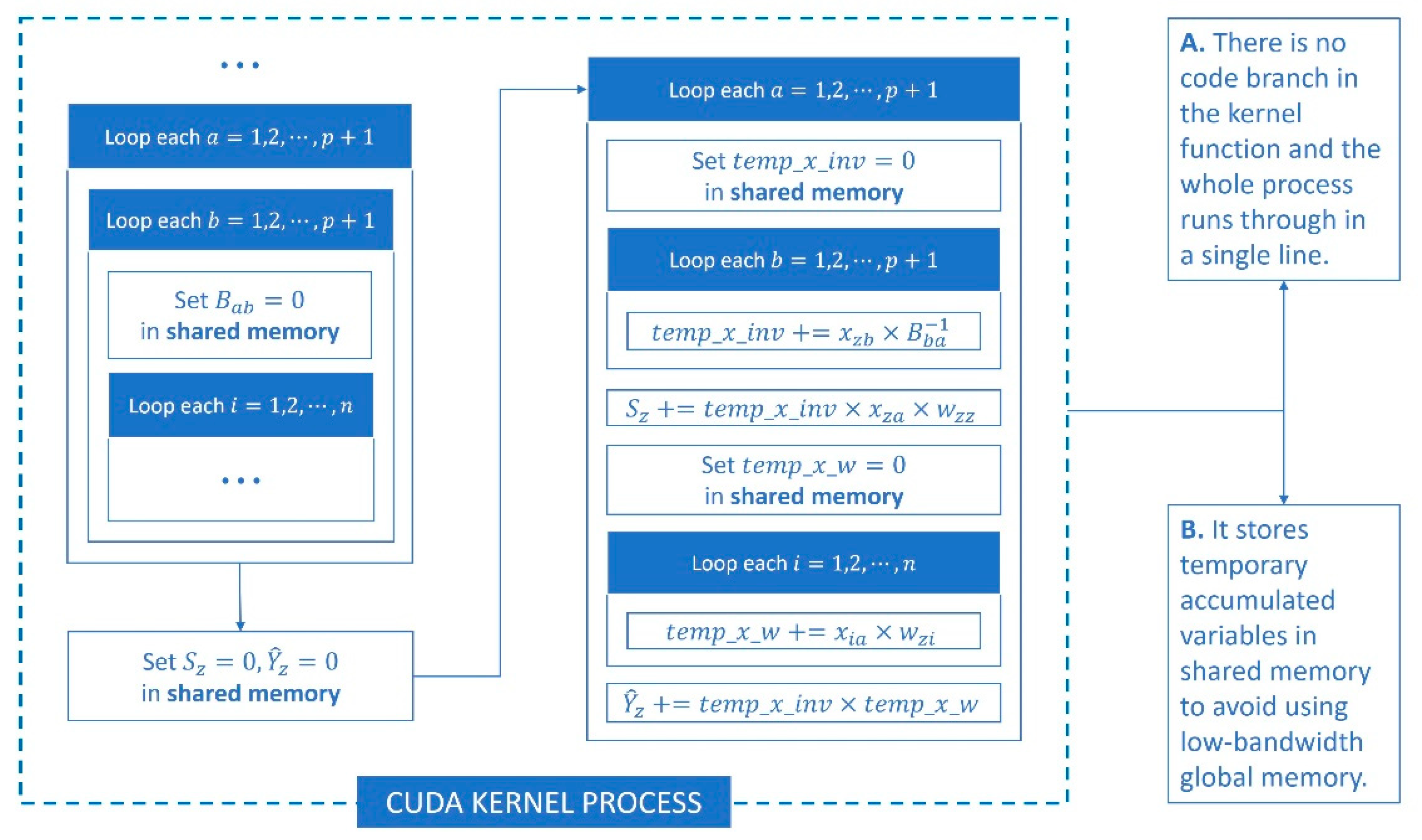
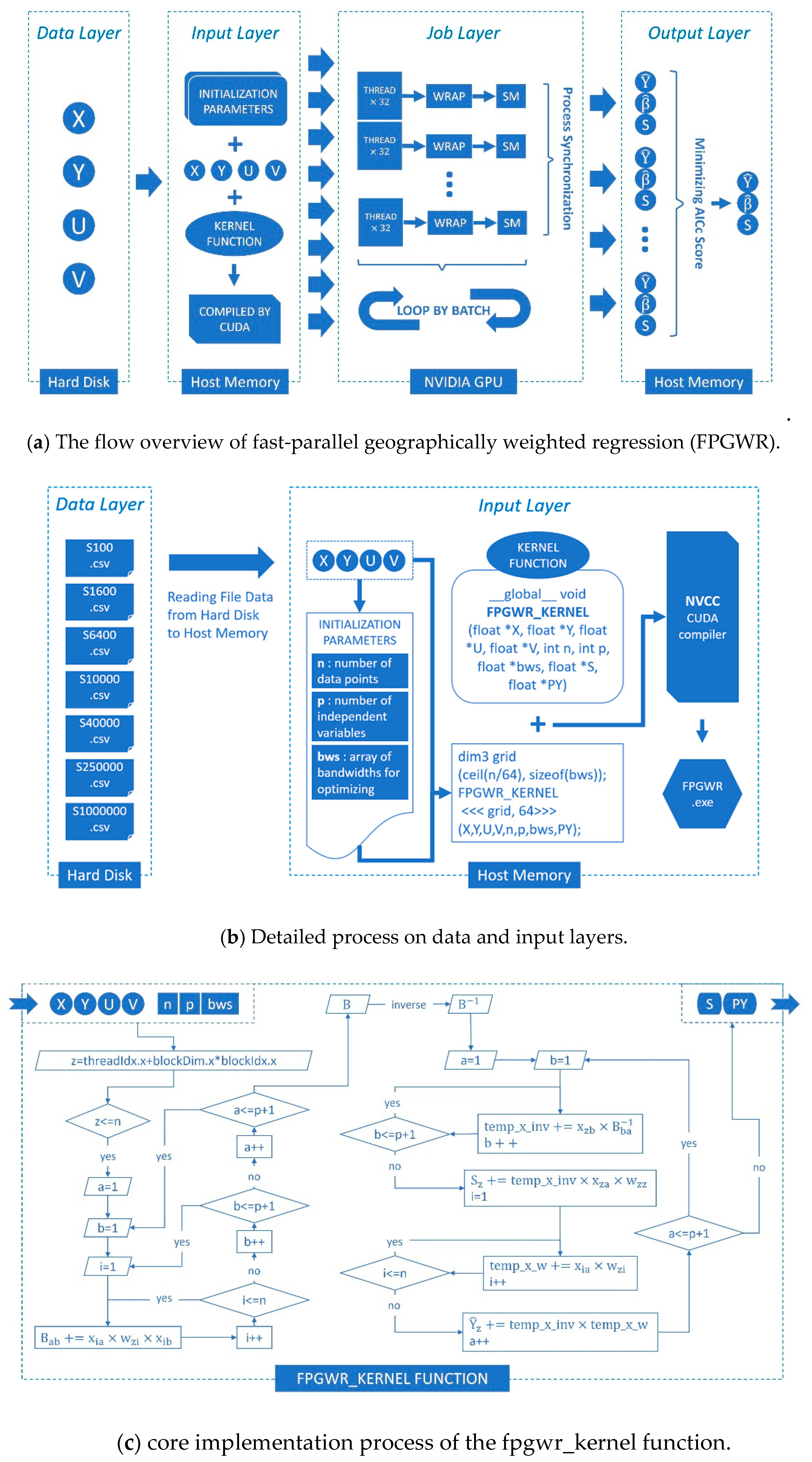
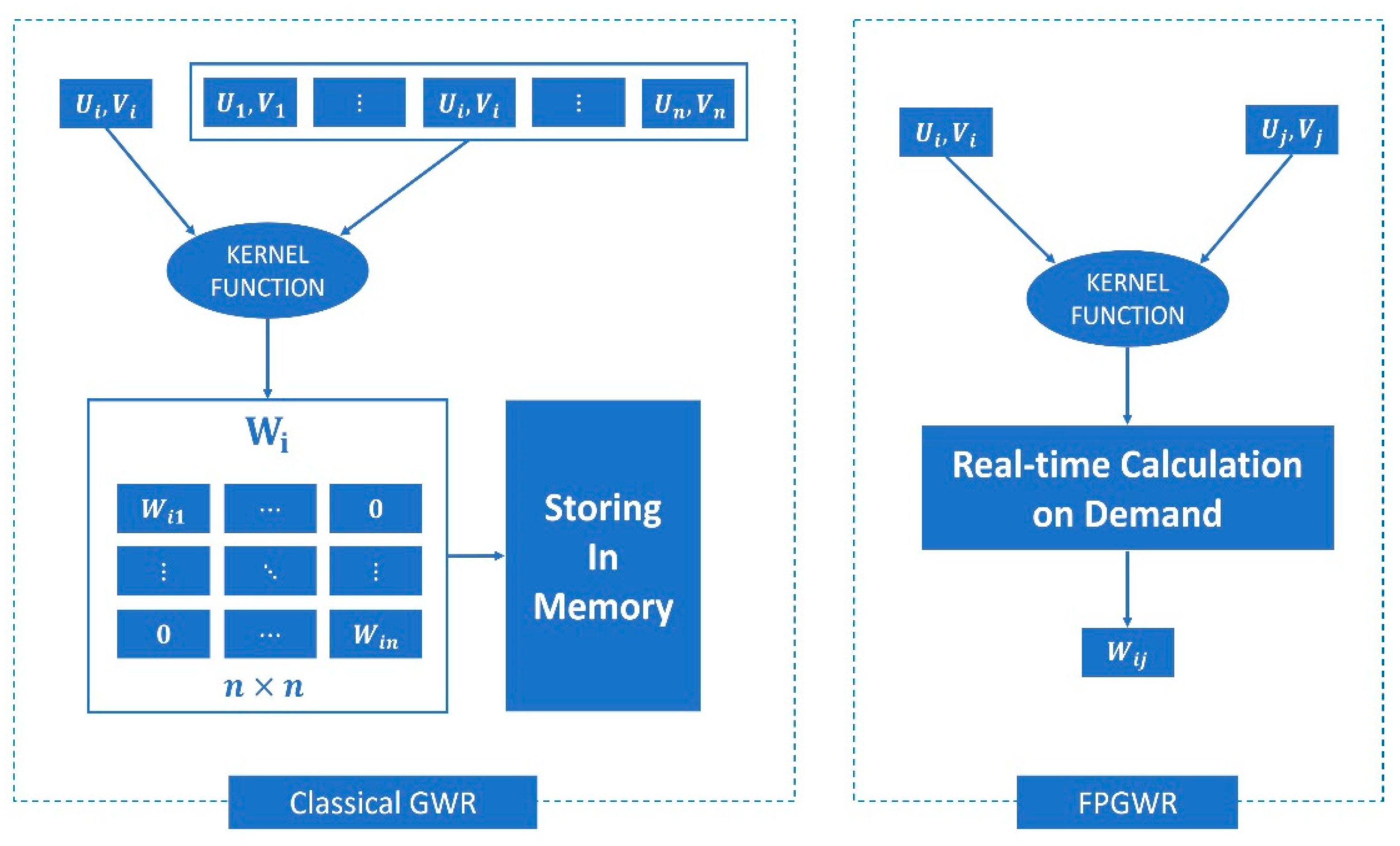
27] studied the implementation of large-scale GWR on an in-memory cluster computing framework Spark (Spark-GWR) and determined that it was a feasible solution using cluster computers to execute GWR in parallel, but great difficulty is encountered for ordinary coders in developing and testing under the cluster environment. As a representative model of local regression, GWR incorporates all of the observations (samples) into the loop of the regression sequence. The key to geographic weighting is the calculation of distance weights for each sample, where it causes costly complexity in terms of runtime and memory. At the same time, the entire process consumes a large amount of computing time because the weight calibrator participates in multilayer loops. Under the condition of large-scale geodata, GWR needs to go through two levels of large cycle iteration, the outer iteration is responsible for point by point regression, and the inner iteration is used for matrix calculation between single sample and full samples. Therefore, limited by data structure and operating mode, GWR is less effective in addressing large-scale geodata. Concurrency methods can improve the efficiency of geographic analysis tools depending on the software optimization, but the hardware parallel environment could obtain native support and achieve the best acceleration performance. Both FastGWR and Spark-GWR could divide GWR into several parallel task sets, and the two parallel programs are designed for CPU architecture that cannot be adapted to GPU architecture. FPGWR decomposes large-scale GWR into simpler parallelizable computing units utilizing atomization algorithm and processes them with numerous parallel GPU cores.
In this paper, we develop FPGWR to reduce the computational complexity in the GWR process and enable GWR’s applications in millions or even tens of millions of geodata. This technique significantly improves the efficiency in regression when utilizing the parallelization of large tasks. On the basis of the CUDA framework, atomic subtasks that are decomposed from large tasks could run on a GPU device in parallel mode. This paper contributes to the prior literature as follows. (1) FPGWR can compensate for the deficiencies of GWR in undertaking regression computation for large-scale geodata, and FPGWR with separate atomic computing units (atomization) is more efficient than GWR. (2) FPGWR is a powerful model for exploring spatial heterogeneity and incorporating high parallelism into geography analysis, which is applicable for studies in various fields, such as economic geography, social science, public health. (3) The improvement from GWR to FPGWR can provide new insights into geospatial computing from spatial and computational perspective.

2. GWR Model and Atomization Algorithm

2.1. GWR Review

Before the 1980s, OLR was frequently applied for geographical phenomena analysis. The predictive coefficients β ^ , calculated by the ordinary least squares (OLS) estimator method, abides by the rule of global optimal unbiased estimation. The final regression result merely reflects the average level in the study region. It is illegitimate to utilize the global regression methods in the local regression model. Therefore, Foster et al. (1986) [28] created a spatial adaptive filter (SAF) learning from varying coefficient modeling, which could describe step-jump and continuous spatial non-stationarity in the coefficients automatically. Based on the local polynomial smoothing technique, Brunsdon et al. (1996) [17] proposed the analysis tool of GWR.

2.1.1. GWR Model

The GWR model extends OLR, introducing the location factor to express the spatial variation of coefficients. In other words, we have the following:
y i = β 0 ( u i , v i ) + m = 1 p β m ( u i , v i ) x i m + ε i i = 1 , 2 , , n
where y i is the regression variable (dependent variable) at location i, ( u i , v i ) represents the coordinate (usually latitude and longitude) of the ith sample point in the study area, β m ( u i , v i ) denotes the kth coefficient of the ith sample point based on a function with independent variables of u i and v i , x i m expresses the mth predictor variable (independent variable), and ε i represents the error term, and n is the sample size. The necessary conditions for Equation (2) can be expressed as follows:
ε i ~ N ( 0 , σ 2 )     C o v ( ε i , ε j ) = 0 ( i j )
For simplicity, Equation (1) is abbreviated as
y i = m = 0 p β i m x i m + ε i i = 1 , 2 , , n     x i 0 1
To prevent GWR from degenerating into a general linear regression, it is necessary that β 1 m = β 2 m = = β n m should not appear in the preconditions.
The variables related to GWR can be defined in the form of matrix. The independent variable matrix X can be calculated by the following form:
X = [ 1 x 11 x 12 x 1 p 1 x 21 x 22 x 2 p 1 x n 1 x n 2 x n p ]

2.1.2. Spatial Weight Kernel Function

There are n terms of spatial weight w i j between two sample points ( i = j is allowed) in the study area. In the GWR model, it is usual to denote the weight matrix W i as a diagonal square matrix:
W i = [ w i 1 0 0 w i n ]
At present, there are several forms of the weight kernel function w i j , and the most used are Bi-Square and Gaussian. The two functions can be expressed as Equations (6) and (7):
Bi Square : w i j = { [ 1 ( d i j b w ) 2 ] 2   , d i j < b w 0         , d i j b w
Gaussian : w i j = e 1 / 2 ( d i j b w ) 2
where d i j represents the distance between two sample points ( i and j ), and b w denotes the bandwidth parameter which could be interpreted as not only the neighbors threshold but also the distance attenuation factor within the weight kernel function.

2.1.3. Model Regression

The regression coefficient estimate β ^ i at position i is defined by
β ^ i = ( X T W i X ) 1 X T W i Y
The regression value Y ^ i of the regression point i based on β ^ i can be estimated from
Y ^ i = X i ( X T W i X ) 1 X T W i Y
where X i represents the ith row vector in matrix X . The hat matrix plays a very important role in the residual analysis of the linear regression model. This study introduces the hat matrix S into GWR. The matrix S can be expressed as follows:
S i = X i ( X T W i X ) 1 X T W i
The regression result matrix Y ^ i can be represented with the hat matrix S :
Y ^ = S Y = [ Y ^ 1 Y ^ n ] = [ S 1 S n ] Y

2.1.4. The Criteria of Optimal Bandwidth Selection

The key to discovering the optimal bandwidth b w is minimizing the A I C c score. Loop selection and golden selection methods are available to obtain the lowest A I C c value. Searching the optimal bandwidth b w is inseparable from the parameter estimation criterion. The criterion A I C c [29] is introduced by Brunsdon et al. (2002) [30] to select the optimal bandwidth of the weight function. The specific formula can be expressed as
A I C c = n ln ( σ ^ 2 ) + n ln ( 2 π ) + n [ n + t r ( S ) n 2 t r ( S ) ]
The residual ε can be calculated by the sample data Y and the regression result Y ^ :
ε = Y Y ^
The unbiased estimate of the random error variance is expressed as σ ^ 2 :
σ ^ 2 = R S S n 2 t r ( S ) + t r ( S T S )
where RSS indicates the sum of squared residuals, t r ( S ) is the trace of the hat matrix S , and n 2 t r ( S ) + t r ( S T S ) represents the effective freedom degree of GWR. In most cases, t r ( S T S ) approximately equals t r ( S ) ( t r ( S T S ) t r ( S ) ), and thereby, the above Equation (14) can be simplified as
σ ^ 2 = R S S n t r ( S )

2.2. Atomizing the GWR Model

As mentioned above, the regression process of the GWR model involves two fixed steps: optimal bandwidth selection and model diagnosis. Most existing packages that have implemented the GWR algorithm are supported by the serial mode. Compared with the parallel mode, the serial mode carries undesirable consequences to the regression computation. The computing containers with noninfinite computational power will be overloaded with too large-scale samples. The runtime arises along with the sample size growth, following a power or even an exponential relationship [31]. In the paper, it is a feasible solution to design the Algorithm 1 (atomization) in reducing the complexity of GWR regression calculation.
Algorithm 1 Atomic Process—The Minimum Unit of Algorithms.
Atomic Process: Optimizing bandwidth searching by minimizing AIC score
  • Given test bandwidth (bw) and atomic process index (z)
  • Calculate   w z z ( w z z 1 ) from Equation (7)
  • Loop   each   a = 1 , 2 , , p + 1 ,   calculate :
  • Loop   each   b = 1 , 2 , , p + 1 ,   calculate :
  • Set   B a b = 0
  • Loop   each   i = 1 , 2 , , n ,   calculate :
  • B a b + = x i a × w z i × x i b
  • End loop
  • End loop
  • End loop
  • Calculate   B 1
  • Set   S z = 0 , Y ^ z = 0
  • Loop   each   a = 1 , 2 , , p + 1 ,   calculate :
  • Set   temp _ x _ inv = 0
  • Loop   each   b = 1 , 2 , , p + 1 ,   calculate :
  • temp _ x _ inv + = x z b × B b a 1
  • End loop
  • S z + = temp _ x _ inv × x z a × w z z
  • Set   t e m p _ x _ w = 0
  • Loop   each   i = 1 , 2 , , n ,   calculate :
  • t e m p _ x _ w + = x i a × w z i
  • End loop
  • Y ^ z + = temp _ x _ inv × t e m p _ x _ w
  • End loop
  • Return   S z , Y ^ z

2.2.1. Intermediate Matrix

In order to introduce the parallel mode legally, we design GWR atomization to decompose the matrix calculation process. The matrix elements used in the result are extracted on-demand to obtain the result value via simple algebraic calculations. It will save huge memory usage and computing resource occupy in the large matrix operation of GWR. Intermediate matrix is an important research object of GWR atomization, which exists in several common models.
OLR can be calculated by the following matrix form:
Y = X β + ε
On basis of OLS, regression coefficient β ^ is estimated from
β ^ = ( X T X ) 1 X T Y
Next, regression result Y ^ of OLR can be expressed as follows:
Y ^ = X ( X T X ) 1 X T Y
By comprehensively analyzing Equations (8), (9), (17), and (18), we can find the intermediate matrix M which exists in all regression models of estimating unbiased via OLS. It can be calculated by the following:
M = ( X T W i X ) 1 X T W i         o r         M = ( X T X ) 1 X T
In the point-by-point regression process, the intermediate matrix M is inevitable.
Matrix X T can be defined by
X T = [ 1 1 1 x 11 x 21 x n 1 x 1 p x 2 p x n p ] .  
where p is the number of independent variables. The multiplication of matrix X T and the diagonal square matrix W i is special. The resulting matrix A can be expressed as follows:
A = X T W i = [ 1 × w i 1 1 × w i 2 1 × w i n x 11 × w i 1 x 21 × w i 2 x n 1 × w i n x 1 p × w i 1 x 2 p × w i 2 x n p × w i n ]
Similarly, matrix B can be written as
B = X T W i X = [ a = 1 p + 1 ( b = 1 p + 1 ( j = 1 n ( x j a × w z j × x j b ) ) ) ] ( p + 1 ) × ( p + 1 )
where matrix B is a square matrix with p + 1 dimensions. In practical applications, p + 1 is usually less than 10, which means that it is legal to ignore the time spent by the inverse operation for matrix B .
Comparing with matrix decomposition, the regression subprocess of GWR relies on the weight matrix W i when calculating matrices A and B . The determination of weighting scheme W i could be achieved: (a) Obtain the coordinate matrix U V ( n × 2 ) of all samples, and then transpose the matrix to matrix U V ( 2 × n ) T . (b) Solve the distance matrix D ( n × n ) between coordinate matrix U V ( n × 2 ) and its transposed matrix U V ( 2 × n ) T . (c) Calculate the weight matrix W ( n × n ) of all samples according to Equation (6) or (7), and then W i is the diagonal matrix formed by the ith row elements of the weight matrix W . However, the process needs huge memory space and calculation time when involving the enormous sample size. In addition, each subprocess of GWR will determine W i once, which causes high redundancy of memory and runtime. The implementation of matrix decomposition approach has been carried out to decrease memory usage and runtime occupation by means of Equations (21) and (22).

2.2.2. Implementation of the Atomization Algorithm

Unlike the large process with full-matrix multiplication, each logically independent subprocess merely participates in the regression calculation once, on the basis of the atomization algorithm. It is the prerequisite for parallelization to ensure that the subprocess is repeatable. To address the problems caused by redundant computing, two aspects (memory and time) of optimization are conducted in the study. The A I C c scores and estimation Y ^ , generated during the bandwidth calibration process, are stored in the singleton pattern. Moreover, by means of on-demand computing, the disadvantage of a high-repetition-rate calculation is eliminated in the large process. Given a test bandwidth b w , the detailed steps of the atomization algorithm can be implemented as Algorithm 1.

3. CUDA Enabled FPGWR

FPGWR based on CUDA has the capability to process massive spatial geodata. The technique is substantially developed to increase the computing speed of GWR. Supported by a large number of SP, the GPU device can handle parallel computing as a natural carrier of HPC. Hardware performs superior to software in terms of the multithread scheduling. Hence, it is the preferred solution to improve GWR on the basis of the CUDA framework.

3.1. Optimizing the Kernel Function of CUDA

CUDA is a general-purpose parallel computing architecture introduced by the NVIDIA Corporation [32]. In the CUDA framework, parallel tasks would be instantiated as independent controllable threads. Independence means that there are no mutually exclusive signals among all threads. Each thread could run synchronously without depending on its sibling threads. Controllability means that the specificity of the thread instances could be controlled by the same parameters. The initialization values are differently set to make the generated instances diverse from each other. Due to the identical computing processes of threads, merely one thread scheduler is needed to manage all threads.
There are two principles for designing the CUDA kernel function to maximize the usage of the GPU scheduling resource and computing cycle. We should minimize the occurrence of WARP Branch in the kernel function as much as possible. At the same time, it is recommended to choose the CUDA memory type flexibly. The specific optimization strategy is shown in Figure 1. By the method of matrix decomposition, the atomic kernel function has successfully prevented process branching. Hence the computation workload can be evened out among the threads. Each atomic task will dynamically be assigned one unique thread index ( z ) that is different from the others. Because the tasks execute in a completely random order, the coupling relationship between the atomic threads and SPs is disconnected. To overcome the performance bottleneck caused by frequent access to global memory, FPGWR utilizes the shared memory to store these temporary variables.

3.2. Implementing FPGWR Based on CUDA

In this study, we have implemented FPGWR in a CUDA framework by utilizing the method of atomization. FPGWR significantly shortens the total time of large-scale GWR regression and releases the memory space of massive spatial matrix data. The FPGWR implementation consists of five steps. Step 1, the program in Host device invokes the GPU device to be prepared, and at the same time, a series of initial parameters are set in the constant memory of the GPU. Step 2, the sample data are input to the global memory of the GPU. The volume of geodata is too enormous to be instantiated in either the shared memory or the local memory. It will throw an “out of memory (OOM)” error when sample data volume is too large to fit in GPU global memory. Step 3, CUDA loads the instructions compiled from the code of the atomic kernel function, and then, the scheduler generates individual threads with the same kernel function. Step 4, all threads are assigned to Streaming Multiprocessor (SM) in the unit of WARP. To address the enormous number of threads, the GPU will activate the flow-shop scheduling mode. Step 5, CUDA feeds back the regression results from the GPU to the Host, and the GPU device resources are released immediately. The detailed workflow of the FPGWR implementation is shown in Figure 2.
As shown in Figure 2a, the FPGWR algorithm could be divided into four layers: data layer, input layer, working layer, and output layer. The data layer is dedicated to storing the files of original observations. The input layer reads the spatial observation data from hard disk into host memory. At the same time, the part of the CUDA programming is instantiated in this layer. The initialization parameters and observation matrices are introduced together into the atomic kernel function, and then, the function will be compiled into an executable program. The working layer runs on the NVIDIA GPU. It starts massive task threads, which are managed uniformly by the multithreaded scheduler of the GPU. At the physical level, WARPs are bundled into a queue of batches, while the WARPs in the same batch are executed synchronously. The output layer is designed to collect the regression results. Based on the bandwidth indexes, these results are organized into multiple sets of regression matrices ( S , Y ^ , and β ^ ). Finally, the algorithm finds the optimal results set that corresponds to the minimum A I C c score.
Figure 2b,c illustrate how the core part of FPGWR works at the micro level. The specific meanings of the initialization parameters ( n , p and b w s ) and the prototype of the FPGWR_KERNEL function are described in Subfigure (b). The detailed process of FPGWR_KERNEL function is presented in Subfigure (c). The steps of the process could correspond to those of Algorithm 1. The multithread scheduling depends on the initial BLOCK and GRID settings of the kernel function in CUDA. BLOCK is set as a one-dimensional vector with a constant value (64), namely, each BLOCK contains 64 threads. GRID is set as a two-dimensional vector, in which the number of the first dimension is the sample size n divided by 64 (number of BLOCK’s first dimension), and the second dimension is the size of the bandwidth array.

4. Results and Discussion

4.1. Data Source

To explore the real performance of FPGWR, three data sources—the simulation dataset, the “Zillow test dataset” [26], and the “Georgia” dataset [33]—are used for the experiment. The simulation dataset is designed to evaluate the influences caused by the sample size and the independent variables size. The “Zillow test dataset” (https://github.com/Ziqi-Li/FastGWR) is assigned to compare the acceleration performance of the different GWR packages. The “Georgia” dataset is used to validate the result accuracy of FPGWR against other schemes.

4.1.1. Simulation Dataset

The test region is displayed as a square area [34] with l length sides, where the sample points are distributed evenly. After setting the sample size of each row to c , the total number of samples could be expressed as n = c × c . The distance between two adjacent samples is calculated by Δ l = l / ( c 1 ) . The lower-left corner is defined as the origin of the coordinate system. The expression for calculating the positions of the samples is given by
( u i , v i ) = ( Δ l × m o d ( i 1 c ) , Δ l × f l o o r ( i 1 c ) )
where mod stands for the remainder function, and floor denotes the rounding function.
The sample data are generated by the GWR model below. It is predefined in Equation (24) as follows:
y i = β 0 ( u i , v i ) + β 1 ( u i , v i ) x i 1 + β 2 ( u i , v i ) x i 2 + β 3 ( u i , v i ) x i 3 + β 4 ( u i , v i ) x i 4 + ε i
To unify the dimensions of the regression coefficients β , all of the values are limited to the interval ( 0 , β m a x ) ( β m a x is a fixed constant). The coefficients β follow 5 functions as follows:
β 0 ( u i , v i ) = 2 β m a x l 2 ( l 2 2 ( l u i ) 2 ( l v i ) 2 )
β 1 ( u i , v i ) = β m a x 2 ( ( sin u i π l ) 2 + ( sin v i π l ) 2 )
β 2 ( u i , v i ) = β m a x 2 ( 2 ( ( tan ( u i π 2 l π 4 ) ) 2 + ( tan ( v i π 2 l π 4 ) ) 2 ) )
β 3 ( u i , v i ) = β m a x e 1 2 l ( ( l 2 u i ) 2 + ( l 2 v i ) 2 )
β 4 ( u i , v i ) = 16 β m a x l 4 ( l 2 4 ( l 2 u i ) 2 ) ( l 2 4 ( l 2 v i ) 2 )
The spatial distribution of the coefficients β is displayed in Figure 3. The five coefficients β selected by the model are closely related to the position of the sample, which demonstrates the spatial non-stationarity of the observations.
According to Formula (27), eight sets of sample datasets are produced for testing. The datasets’ construction parameters and resource link are exhibited in Table 1.

4.1.2. Zillow Test Dataset

The “Zillow test dataset” [26] is a subset of the Zillow property dataset, which consists of the single-family housing information within the metropolitan area of Los Angeles. The mathematical expression of the dataset is expressed as Equation (30). The dataset is open source on GitHub along with the FastGWR algorithm (https://github.com/Ziqi-Li/FastGWR). This paper has downloaded eight datasets (1 k, 2 k, 5 k, 10 k, 15 k, 20 k, 50 k and 100 k) from the GitHub repository for the comparative experiment.
V a l u e i = β i 0 + β i 1 A r e a i + β i 2 N b a t h s i + β i 3 N b e d s i + β i 4 A g e i + ε i

4.1.3. Georgia Dataset

The Georgia dataset [33] contains a subset (socio-demographic characteristics) of the 1990 US census within the state of Georgia. The coordinates of the data points are set at the centroids of counties, so there are 159 records containing county population attributes in the dataset. The model could be defined as Equation (31):
P c t B a c h = β 0 + β 1 I n t e r c e p t + β 2 P c t P o v + β 3 P c t R u r a l + β 4 P c t B l a c k + ε

4.2. Testing Specifications and Environment

The experiment for FPGWR is conducted on a desktop computer. The configuration of this computer is an Intel i7-9700K 3.60 GHz 8-core CPU (Intel Corporation, Santa Clara, CA, USA), 16 GB Random Access Memory (RAM) (Kingston Technology Corporation, Fountain Valley, CA, USA) and NVIDIA GeForce RTX 2080 Ti 11 GB GPU (NVIDIA Corporation, San Tomas Expressway Santa Clara, CA, USA). In addition, it has installed version 10.2.95 of the CUDA development kit, version 14.0.25431.01 Update 3 of Microsoft Visual Studio 2015 (development IDE), and the Microsoft Windows 10.0.17134 Professional Edition operating system (OS). Note that 4352 SP core units are placed in the GPU device. Relying on its ultra-high-speed task scheduling capability, the GPU can withstand the pressure of multithreaded computation tasks in parallel.

4.3. Results

4.3.1. FPGWR Performance

Due to the transformation of parallelization, the regression efficiency of FPGWR increases dramatically against GWR. The bandwidth optimization is clearly a repetitive process. To compare the acceleration performances, this study analyzes only the single subprocess with a fixed bandwidth. The runtimes of FPGWR with different sample sizes are shown in Table 2. Given four independent variables, the runtime can be controlled within 2 s when the sample size is less than 40 k. After increasing the sample size to 250 k, the runtime becomes approximately 66.6 s. As the sample size increases to the millions scale, it spends only approximately 1094.7 s. The result shows that the runtime obeys a logarithmic variation rule as the sample size changes.
The runtimes vary tremendously with different sample sizes. To enable the display of all results together, the y-axis of the logarithmic scale is plotted in Figure 4. The comprehensive analysis of Table 2 and Figure 4 reveals that both the sample size and the number of independent variables can influence the variation of runtime. The regression time has positive association with the number of independent variables. When the sample size varies, the variation in the runtime is similar with different numbers of independent variables. Given the same sample size, the results on the time exhibit a simple multiple relationship among the different numbers of independent variables. In summary, the sample size has a more pronounced impact than the number of independent variables on the regression time.
Speed-up and efficiency are important metrics for the performance check of parallel algorithms [35]. Speed-up refers to the ratio of single processor runtime to multiprocessor runtime, and efficiency represents the average of speed-up in multiprocessors [36]. The speed-up of FPGWR relies on the GPU performance, which consists of SP number, base clock frequency, and memory bandwidth. Table 3 compares the performance configuration of different type GPUs. On basis of the 250,000 simulation samples, this study regresses the model given in equation (24) with an increasing number of GPU cores. The runtime of GTX1050 is set as the benchmark value to calculate the speed-up factor of GPUs with different SP numbers. The speed-ups growth proves that FPGWR has an outstanding parallel scalability. Figure 5 illustrates that the computation time decreases approximate-linearly as the number of GPU cores increases. It exhibits an obvious positive linear relationship between efficiency and GPU cores.
The experimental result demonstrates the outstanding capability of FPGWR to accelerate GWR, although its performance varies slightly among different orders of magnitude of observations. By setting appropriate sample sizes and independent variable numbers, the full potential of FPGWR can be achieved in various fields.

4.3.2. Comparison of FPGWR and Other GWR

Benefiting from the development of computer hardware, researchers could quickly and easily build the GPU environment for large-scale spatial study. To verify the acceleration capability, another four GWR—namely, FastGWR (Python), MGWR (Python), GWmodel (R), and spgwr (R)—are selected to compare with FPGWR. The test data utilized by the experiment is the “Zillow test dataset.” GWmodel uses moving window weighting technique to decrease the computation. FastGWR implements distributed parallelism in HPC environment to improve operating efficiency. FastGWR is superior than MGWR, GWmodel and spgwr in terms of overall calculating efficiency. As a side note, although the optimal environment for FastGWR is an HPC cluster, it is more unbiased to conduct the experiments based on a single desktop environment.
The runtimes of the five packages with different sample sizes are displayed in Table 4. The runtime merely contains the single regression time with a specified bandwidth (as in Section 4.3.1). Given 1000 observations, FPGWR is 5 times faster than FastGWR, 32 times faster than MGWR, 88 times faster than GWmodel, and 865 times faster than spgwr. As the sample size increases to 10,000, FPGWR is approximately 14 times faster than FastGWR, approximately 157 times faster than MGWR, approximately 2185 times faster than GWmodel, and approximately 45,811 times faster than spgwr. Once the sample size exceeds 20,000, spgwr will fail to complete the regression task first, followed by GWmodel and MGWR. The cause is that the three schemes fail to avoid storing the high-dimensional weight matrix and other intermediate matrices.
The runtimes of the five packages are illustrated in Figure 6. The y-axis is marked on a logarithmic scale to display all of the results together. Observing each package separately reveals that the runtimes of the five schemes all exhibit a logarithmic increasing trend. According to Figure 6, the performances of the five packages are enhanced generation by generation. FPGWR is the most ideal implementation among these schemes.
Overall, FPGWR is a feasible GWR accelerator with a low development cost and simple productization process. Compared with other packages, FPGWR can greatly simplify a complicated job through decomposing the redundant full-sample regression.

4.3.3. Validation of the Result Accuracy

To validate the accuracy of FPGWR against other GWR packages, the results ( β ^ , A d j . R 2 and A I C c scores) of the five packages are compared based on the well-known “Georgia” dataset. The dependent variable PctBach and independent variables Intercept, PctPov, PctRural and PctBlack are chosen to calibrate the same GWR model according to Equation (31). On the basis of the adaptive Bi-square kernel function, 93 nearest neighbors are selected for the optimal bandwidth. As shown in Table 5, the Mean and Standard Deviation of the estimated coefficients β ^ are displayed in the middle section, and the A d j . R 2 and A I C c scores are indicated in the lower section. The FPGWR result is clearly consistent with those of the other four packages.
The spatial distribution of the estimated coefficients β ^ in the study area is illustrated in Figure 7. To simulate the spatial variation better, both the surfaces are interpolated as a continuous surface utilizing the griddata method.

4.4. Discussion

Multiple loops are necessary in the GWR model until FPGWR atomizes the large process. Enormous calculation redundancy would inevitably emerge in the implementation of the GWR algorithm. The algorithm structure is nested with multilevel loops, where the upper loop depends on the lower loop and the internal sequence of each loop is fixed. It is illegitimate to disturb the original iterative sequence of the subprocesses; otherwise, the accuracy of the regression results would be questioned seriously. FPGWR introduces a hybrid (parallel–serial) mode, which could enable the GPU device to not only tolerate parallel tasks of each batch but also complete all of the tasks efficiently. The subprocesses could be randomly executed without errors, and the accuracy of the results is guaranteed for the model diagnosis. FPGWR differs obviously from GWR in its memory usage and time cost.

4.4.1. Memory

The matrix storage strategy of GWR is different from FPGWR, as shown in Figure 8. The FPGWR optimizes the storage mode in utilizing the schemes, the on-demand storage and the matrix vectorization. The weight matrix W i is stored as an n × n diagonal matrix in the GWR model. Although only the diagonal elements must be solved, a storage space of size n 2 is demanded. The memory complexity could be expressed as O ( n 2 ) . In the subsequent steps, the calculations of the matrices B , B 1 and A all inherit the memory complexity. In comparison, the FPGWR method only stores the data as required. Its memory complexity can be reduced into O ( ( p + 1 ) n ) ( p + 1 10 in common).
Table 6 illustrates the comparison of memory usage between FPGWR and GWR. When the sample size is less than 100,000, the memory of the GPU device is still available for usage. Once the size is increased to 10,000,000, GWR approximately requires 364 TB RAM. Any existing single GPU device could not allocate so much storage space. In contrast, FPGWR consumes only 380 MB RAM. To summarize, FPGWR demonstrates a tremendous advantage over GWR.
.

4.4.2. Time

It is necessary for the process of calculating the hat matrix S in GWR. The weight matrix W i is a special diagonal matrix that does not increase the runtime complexity during matrix multiplication. The runtime complexity of matrices A is O ( 1 ) , and the runtime complexity of B is O ( ( p + 1 ) 2 n ) . Because p + 1 is far less than n , the computing time of matrix B can be ignored. Given a fixed weight bandwidth, the runtime complexity of hat matrix S i can be expressed as O ( ( p + 1 ) 2 n ) . After n operations on S i , the runtime complexity of matrix S is defined by O ( ( p + 1 ) 2 n 2 ) . Different GWR schemes utilize varied ways to select the optimal bandwidth, and thereby, the study will omit a discussion about the runtime complexity of the whole process. The regression subprocess of single sample is appropriate to be used for the runtime analysis in this subsection. Instead of computing iteratively, FPGWR atomizes the regression process of each point as an independent thread. The strategy has reduced the runtime complexity of matrix S appreciably. At the same time, the runtime complexity of matrix of A becomes O ( ( p + 1 ) n ) , and the runtime complexity of matrix of B becomes O ( ( p + 1 ) 2 n ) . By combining matrices A and B in the form of parallel addition, the hat matrix S i gains a runtime complexity of O ( ( p + 1 ) ( p + 2 ) n ) . The runtime complexity of FPGWR is theoretically lower than GWR, but the instruction operation efficiency of host device differs significantly from the GPU device, and the methods used by the different libraries to optimize the matrix operation are inconsistent. Therefore, the actual comparison results should refer to the experimental results (in Section 4.3.2).
The achievement of GWR regression coefficients requires consuming much time for repeated iteration when handling big geodata. For example, when the sample size is 1,000,000, single point regression of GWR needs to be iterated for 1,000,000 times with a huge time occupying and memory usage. Therefore, this problem could be solved by parallelization strategy. The atomization algorithm does not store the weight matrix and other temporary matrices during each point regression iteration, but only reads and calculates the matrix elements on-demand. FPGWR shortens computation time while using much less memory space through parallelizing these atomic units on CUDA.

5. Conclusions

GWR is a local modeling technique that has been widely used in various disciplines. However, GWR has significant computational redundancy and can handle approximately 15,000 geographical observations at most. To apply the local smoothing technique on a large-scale spatial dataset, we proposed an improved algorithm FPGWR to solve these problems. FPGWR optimizes the matrix storage mode to overcome the limitation on memory space, thereby significantly reducing the memory complexity of GWR. Furthermore, it introduces a parallel computing mode, decomposing the full-sample large cycle into an atomization process, to decrease the runtime complexity substantially.
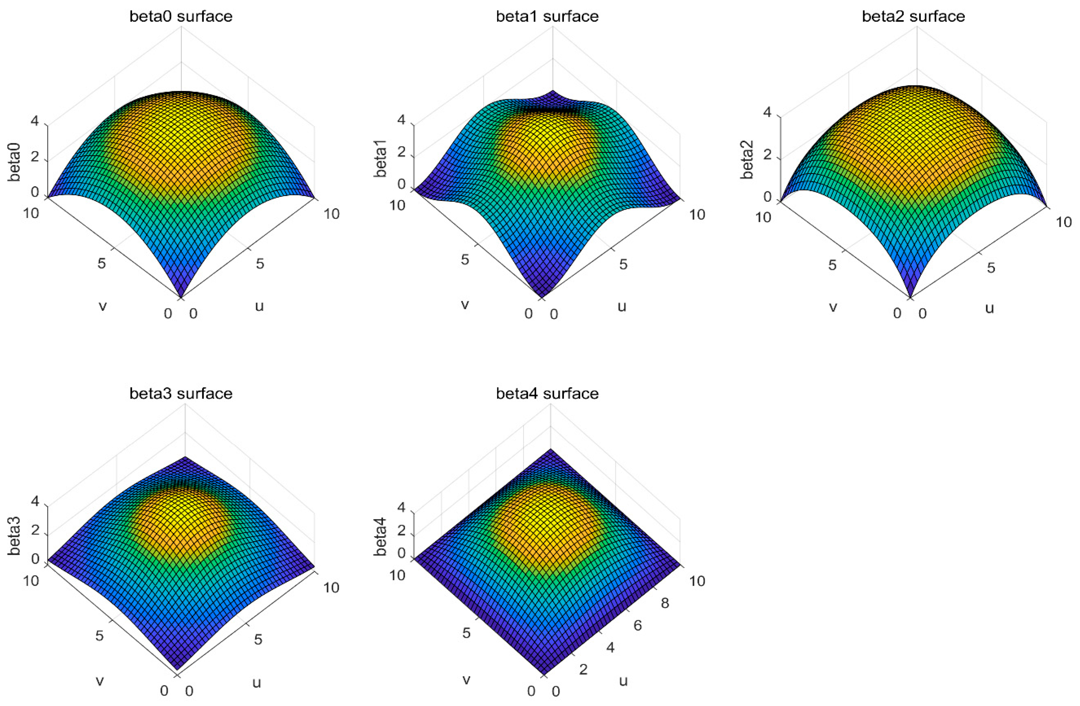
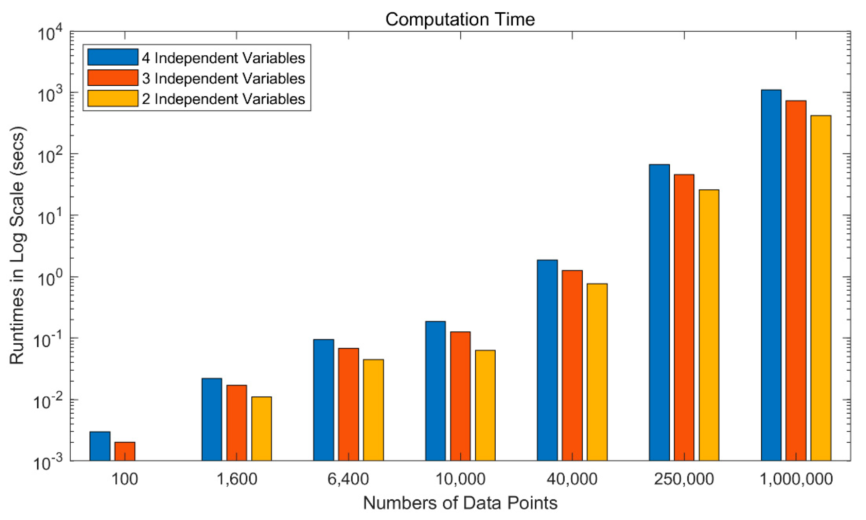
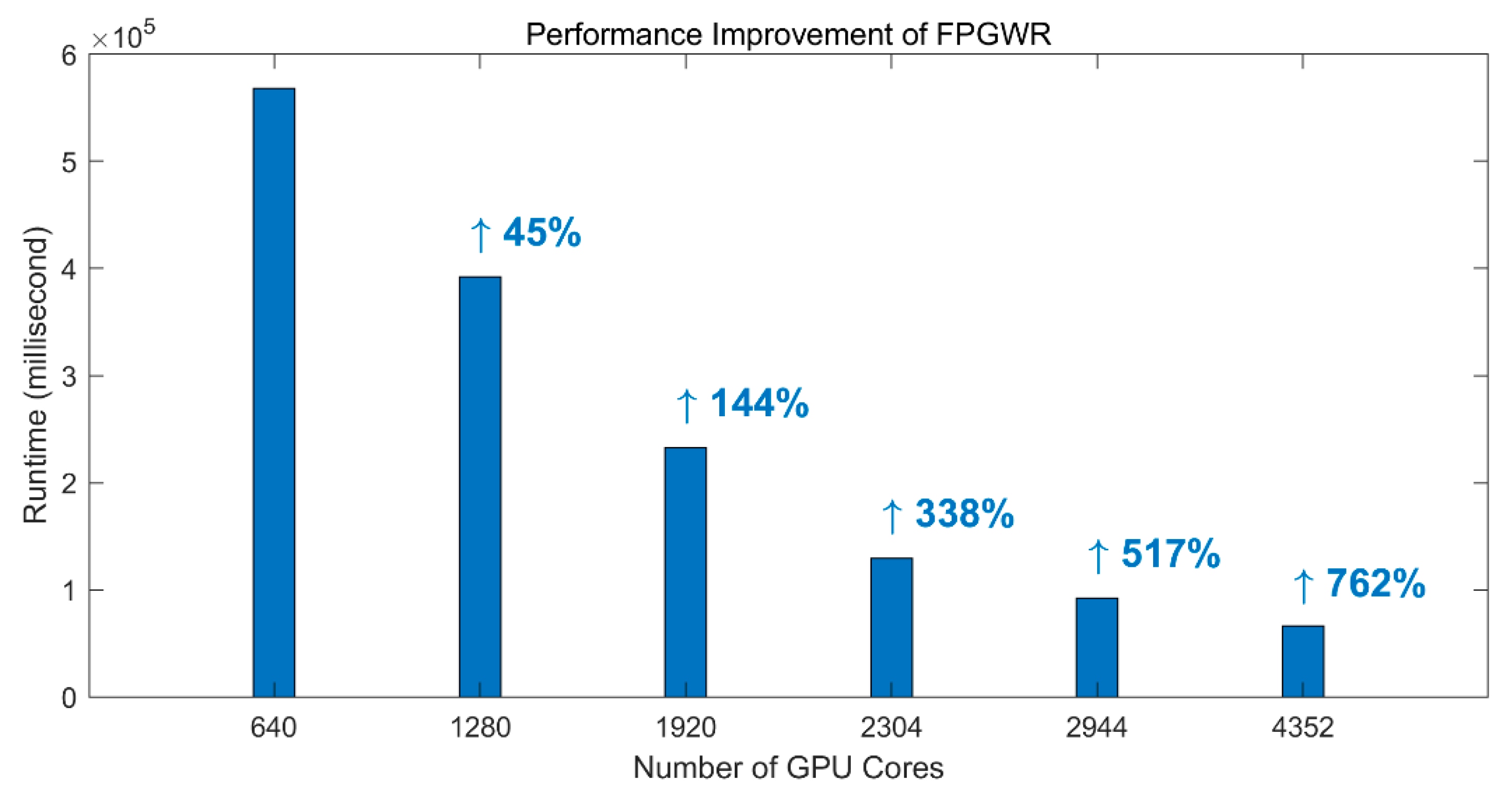
To demonstrate the practicability of FPGWR, simulation and Zillow datasets are used to conduct the experiment. The results show that the regression runtime is exponentially related to the number of observations, and thus, GWR is unable to process the regression task with large volumes of geodata. In comparison, the time taken up by FPGWR exhibits a logarithmic relationship with the number of observations; hence, FPGWR represents a significant advance in handling the massive geodata mining task.
In summary, the dilemma that limits GWR in the data scale could be considerably alleviated by FPGWR, and thus, the application domains of GWR would be potentially expanded to a large extent. Under these circumstances, increasingly large datasets from geographical or nongeographical fields could be converted to the providers of the large-scale geographic analysis services. In the future, we will investigate a key issue: how to adapt FPGWR to non-CUDA architectures, even other non-GPU HPC devices, to enhance the versatility of the extended algorithm.

Author Contributions

Conceptualization, Dongchao Wang, and Yi Yang; Methodology, Dongchao Wang; Resources, Dongchao Wang; Software, Dongchao Wang; Validation, Dongchao Wang; Writing—original draft, Dongchao Wang; Writing—review and editing, Dongchao Wang, Yi Yang, Agen Qiu, Xiaochen Kang, Jiakuan Han, and Zhengyuan Chai. All authors have read and agreed to the published version of the manuscript.

Funding

This research was funded by the National Key Research and Development Project (grant number 2019YFB2102500/2019YFB2102503), the National Natural Science Foundation of China (grant number 71903183, 41801316, 41701461), and the Basic Scientific Research Fund of CASM (grant number AR1910).

Conflicts of Interest

The authors declare no conflict of interest.

References

  1. Toch, E.; Lerner, B.; Ben-Zion, E.; Ben-Gal, I. Analyzing large-scale human mobility data: A survey of machine learning methods and applications. Knowl. Inf. Syst. 2019, 58, 501–523. [Google Scholar] [CrossRef]
  2. Weckström, C.; Kujala, R.; Mladenović, M.N.; Saramäki, J. Assessment of large-scale transitions in public transport networks using open timetable data: Case of Helsinki metro extension. J. Transp. Geogr. 2019, 79, 102470. [Google Scholar] [CrossRef]
  3. Hicks, J.L.; Althoff, T.; Sosic, R.; Kuhar, P.; Bostjancic, B.; King, A.C.; Leskovec, J.; Delp, S.L. Best practices for analyzing large-scale health data from wearables and smartphone apps. NPJ Digit. Med. 2019, 2, 1–12. [Google Scholar] [CrossRef]
  4. Tasar, O.; Tarabalka, Y.; Alliez, P. Incremental learning for semantic segmentation of large-scale remote sensing data. IEEE J. Sel. Top. Appl. Earth Obs. Remote Sens. 2019, 12, 3524–3537. [Google Scholar] [CrossRef] [Green Version]
  5. Li, Z.; Huang, Q.; Jiang, Y.; Hu, F. SOVAS: A scalable online visual analytic system for big climate data analysis. Int. J. Geogr. Inf. Sci. 2020, 34, 1188–1209. [Google Scholar] [CrossRef]
  6. Miller, H.J.; Goodchild, M.F. Data-driven geography. GeoJournal 2015, 80, 449–461. [Google Scholar] [CrossRef]
  7. Xia, J.; Huang, S.; Zhang, S.; Li, X.; Lyu, J.; Xiu, W.; Tu, W. DAPR-tree: A distributed spatial data indexing scheme with data access patterns to support Digital Earth initiatives. Int. J. Digit. Earth 2020, 1–16. [Google Scholar] [CrossRef]
  8. Aji, A.; Wang, F.; Vo, H.; Lee, R.; Liu, Q.; Zhang, X.; Saltz, J. Hadoop-GIS: A high performance spatial data warehousing system over MapReduce. In Proceedings of the VLDB Endowment International Conference on Very Large Data Bases, Trento, Italy, 26–30 August 2013; Volume 6. [Google Scholar]
  9. Wu, Q.Y.; Su, K.Y.; Zou, Z.J. A mapreduce-based method for parallel calculation of bus passengers origin and destination from massive transit data. J. Geo Inf. Sci. 2018, 20, 647–655. [Google Scholar]
  10. Wilkinson, B.; Allen, M. Parallel Programming; Prentice Hall: Upper Saddle River, NJ, USA, 1999. [Google Scholar]
  11. Gong, Z.; Tang, W.; Bennett, D.A.; Thill, J.-C.F. Parallel agent-based simulation of individual-level spatial interactions within a multicore computing environment. Int. J. Geogr. Inf. Sci. 2013, 27, 1152–1170. [Google Scholar] [CrossRef]
  12. Tang, W.; Feng, W.; Jia, M. Massively parallel spatial point pattern analysis: Ripley’s K function accelerated using graphics processing units. Int. J. Geogr. Inf. Sci. 2015, 29, 412–439. [Google Scholar] [CrossRef]
  13. Zhang, G.; Zhu, A.X.; Huang, Q. A GPU-accelerated adaptive kernel density estimation approach for efficient point pattern analysis on spatial big data. Int. J. Geogr. Inf. Sci. 2017, 31, 2068–2097. [Google Scholar] [CrossRef]
  14. Sandric, I.; Ionita, C.; Chitu, Z.; Dardala, M.; Irimia, R.; Furtuna, F.T. Using CUDA to accelerate uncertainty propagation modelling for landslide susceptibility assessment. Environ. Model. Softw. 2019, 115, 176–186. [Google Scholar] [CrossRef]
  15. Stojanovic, N.; Stojanovic, D. Parallelizing multiple flow accumulation algorithm using cuda and openacc. ISPRS Int. J. Geo Inf. 2019, 8, 386. [Google Scholar] [CrossRef] [Green Version]
  16. Pei, T.; Song, C.; Guo, S.; Shu, H.; Liu, Y.; Du, Y.; Ma, T.; Zhou, C. Big geodata mining: Objective, connotations and research issues. J. Geogr. Sci. 2020, 30, 251–266. [Google Scholar] [CrossRef]
  17. Brunsdon, C.; Fotheringham, A.S.; Charlton, M.E. Geographically weighted regression: A method for exploring spatial nonstationarity. Geogr. Anal. 1996, 28, 281–298. [Google Scholar] [CrossRef]
  18. Zhang, P.; Yang, D.; Zhang, Y.; Li, Y.; Liu, Y.; Cen, Y.; Zhang, W.; Geng, W.; Rong, T.; Liu, Y.; et al. Re-examining the drive forces of China’s industrial wastewater pollution based on GWR model at provincial level. J. Clean. Prod. 2020, 262, 121309. [Google Scholar] [CrossRef]
  19. Wu, D. Spatially and Temporally Varying Relationships between Ecological Footprint and Influencing Factors in China’s Provinces Using Geographically Weighted Regression (GWR). J. Clean. Prod. 2020, 261, 121089. [Google Scholar] [CrossRef]
  20. Yuan, Y.; Cave, M.; Xu, H.; Zhang, C. Exploration of spatially varying relationships between Pb and Al in urban soils of London at the regional scale using geographically weighted regression (GWR). J. Hazard. Mater. 2020, 393, 122377. [Google Scholar] [CrossRef]
  21. Hong, I.; Yoo, C. Analyzing Spatial Variance of Airbnb Pricing Determinants Using Multiscale GWR Approach. Sustainability 2020, 12, 4710. [Google Scholar] [CrossRef]
  22. Wu, S.; Wang, Z.; Du, Z.; Huang, B.; Zhang, F.; Liu, R. Geographically and temporally neural network weighted regression for modeling spatiotemporal non-stationary relationships. Int. J. Geogr. Inf. Sci. 2020, 1–27. [Google Scholar] [CrossRef]
  23. Bivand, R.; Yu, D.; Nakaya, T.; Garcia-Lopez, M.A. Package SPGWR; R Software Package; R Foundation for Statistical Computing: Vienna, Austra, 2020. [Google Scholar]
  24. Gollini, I.; Lu, B.; Charlton, M. GWmodel: An R Package for Exploring Spatial Heterogeneity Using Geographically Weighted Models. J. Stat. Softw. 2015, 63, 1–50. [Google Scholar] [CrossRef] [Green Version]
  25. Oshan, T.M.; Li, Z.; Kang, W.; Wolf, L.J.; Fotheringham, A.S. mgwr: A Python implementation of multiscale geographically weighted regression for investigating process spatial heterogeneity and scale. ISPRS Int. J. Geo Inf. 2019, 8, 269. [Google Scholar] [CrossRef] [Green Version]
  26. Li, Z.; Fotheringham, A.S.; Li, W.; Oshan, T. Fast Geographically Weighted Regression (FastGWR): A scalable algorithm to investigate spatial process heterogeneity in millions of observations. Int. J. Geogr. Inf. Sci. 2019, 33, 155–175. [Google Scholar] [CrossRef]
  27. Tran, H.T.; Nguyen, H.T.; Tran, V.T. Large-scale geographically weighted regression on Spark. In Proceedings of the 2016 Eighth International Conference on Knowledge and Systems Engineering (KSE), Hanoi, Vietnam, 6–8 October 2016; pp. 127–132. [Google Scholar]
  28. Foster, S.A.; Gorr, W.L. An adaptive filter for estimating spatially-varying parameters: Application to modeling police hours spent in response to calls for service. Manag. Sci. 1986, 32, 878–889. [Google Scholar]
  29. Akaike, H. A new look at the statistical model identification. IEEE Trans. Autom. Control 1974, 19, 716–723. [Google Scholar]
  30. Brunsdon, C.; Fotheringham, A.S.; Charlton, M. Geographically weighted summary statistics—A framework for localised exploratory data analysis. Comput. Environ. Urban Syst. 2002, 26, 501–524. [Google Scholar] [CrossRef] [Green Version]
  31. Harris, R.; Singleton, A.; Grose, D.; Brundson, C.; Longley, P. Grid-enabling geographically weighted regression: A case study of participation in higher education in England. Trans. GIS 2010, 14, 43–61. [Google Scholar]
  32. NVIDIA Corporation. Compute Unified Device Architecture (CUDA). Available online: https://developer.nvidia.com/cuda-toolkit (accessed on 6 October 2020).
  33. Fotheringham, A.S.; Brunsdon, C.; Charlton, M. Geographically Weighted Regression: The Analysis of Spatially Varying Relationships; John Wiley & Sons: Hoboken, NJ, USA, 2002. [Google Scholar]
  34. Zhang, H.; Mei, C. Local least absolute deviation estimation of spatially varying coefficient models: Robust geographically weighted regression approaches. Int. J. Geogr. Inf. Sci. 2011, 25, 1467–1489. [Google Scholar]
  35. Eager, D.L.; Zahorjan, J.; Lazowska, E.D. Speedup versus efficiency in parallel systems. IEEE Trans. Comput. 1989, 38, 408–423. [Google Scholar]
  36. Yang, L.; Sun, X.; Li, Z. An efficient framework for remote sensing parallel processing: Integrating the artificial bee colony algorithm and multiagent technology. Remote Sens. 2019, 11, 152. [Google Scholar] [CrossRef] [Green Version]
Figure 1. Optimizing the compute unified device architecture (CUDA) kernel function.
Ijgi 09 00653 g001
Figure 2. Flow diagram of FPGWR on CUDA (ac).
Ijgi 09 00653 g002
Figure 3. Coefficient ( β 0 , β 1 , β 2 , β 3 and β 4 ) surface.
Ijgi 09 00653 g003
Figure 4. Runtime comparison (bar) for different numbers of coefficients using different numbers of data points.
Ijgi 09 00653 g004
Figure 5. Performance comparison of FPGWR for an increasing number of GPU cores.
Ijgi 09 00653 g005
Figure 6. Runtime comparison (bar) for different packages using different numbers of data points.
Ijgi 09 00653 g006
Figure 7. Surfaces of coefficient estimates.
Ijgi 09 00653 g007
Figure 8. Different storage modes of weight matrix between classical GWR and FPGWR.
Ijgi 09 00653 g008
Table 1. Construction parameters of example data and access entrance of resource.
l c β m a x x m a x σ Number of Data Points
1010420.5100
1040420.51600
1080420.56400
10100420.510,000
10200420.540,000
10500420.5250,000
101000420.51,000,000
102000420.54,000,000
Note: Resource URL: https://pan.baidu.com/s/1c0Ga8Ngej0SG990sdxHQ_A. Access code: 8dve.
Table 2. Runtime (in seconds) for different numbers of coefficients using different numbers of data points.
Number of Data PointsFour Independent VariablesThree Independent VariablesTwo Independent Variables
1000.0030.0020.001
16000.0220.0170.011
64000.0950.0680.045
10,0000.1860.1260.063
40,0001.8671.2560.766
250,00066.61646.38626.154
1,000,0001094.654738.636421.922
Table 3. Performance comparison for different types of graphics processing unit (GPU).
Type of NVIDIA GPUSP NumberBase Clock Frequency (MHz)Memory Bandwidth (GB/s)Runtime (ms)Speed-Up Factor
GTX 1050640135484568,0861
GTX 106012801506192391,9681.45
GTX 107019201506256232,8012.44
RTX 207023041410448129,6654.38
RTX 20802944151544892,1416.17
RTX 2080 Ti4352135061665,9168.62
Table 4. Runtime (in seconds) for five GWR packages using different numbers of data points.
Number of Data PointsFPGWRFastGWRMGWRGWmodelSpgwr
10000.010.050.320.888.65
20000.020.130.954.1260.26
50000.060.475.4353.151095.80
10,0000.182.4528.34393.308245.93
15,0000.274.4258.971464.12n/a
20,0000.506.76n/an/an/a
50,0002.7264.57n/an/an/a
100,00010.80307.12n/an/an/a
Table 5. Statistical results of local coefficient estimates and regression estimates for five GWR packages.
VariablesFPGWRFastGWRMGWRGWmodelSpgwr
Mean
Standard Deviation
Intercept 23.074823.074823.074823.074823.0748
4.10484.10484.10484.10484.1048
PctPov −0.2625−0.2625−0.2625−0.2625−0.2625
0.09160.09160.09160.09160.0916
PctRural −0.1181−0.1181−0.1181−0.1181−0.1181
0.03700.03700.03700.03700.0370
PctBlack 0.04450.04450.04450.04450.0445
0.05760.05760.05760.05760.0576
PctBach 10.936310.936310.936310.936310.9363
4.34894.34894.34894.34894.3489
Value
Adj . R 2 0.58120.58120.58120.58120.5812
AICc 896.35896.35896.35896.35896.35
Table 6. The comparison of memory usage for FPGWR against classical GWR.
Number of Data PointsFPGWRClassical GWR
1003.9 KB39 KB
100039 KB3.8 MB
10,000390 KB380 MB
100,0003.8 MB38 GB
1,000,00038 MB3.8 TB
10,000,000380 MB364 TB
Note: 32-bit floats were used for all decimals and p = 9 .
Publisher’s Note: MDPI stays neutral with regard to jurisdictional claims in published maps and institutional affiliations.

