A Continuous, Semi-Automated Workflow: From 3D City Models with Geometric Optimization and CFD Simulations to Visualization of Wind in an Urban Environment

Abstract

The concept and implementation of Smart Cities is an important approach to improve decision making as well as quality of life of the growing urban population. An essential part of this is the presentation of data from different sources within a digital city model. Wind flow at building scale has a strong impact on many health and energy issues in a city. For the analysis of urban wind, Computational Fluid Dynamics (CFD) has become an established tool, but requires specialist knowledge to prepare the geometric input during a time-consuming process. Results are available only as predefined selections of pictures or videos. In this article, a continuous, semi-automated workflow is presented, which ❶ speeds-up the preparation of CFD simulation models using a largely automated geometry optimization; and ❷ enables web-based interactive exploration of urban wind simulations to a large and diverse audience, including experts and layman. Results are evaluated based on a case study using a part of a district in Stuttgart in terms of: ➀ time saving of the CFD model preparation workflow (85% faster than the manual method), ➁ response time measurements of different data formats within the Smart City platform (3D Tiles loaded 30% faster than geoJSON using the same data representations) and ➂ protocols (3DPS provided much higher flexibility than static and 3D container API), as well as ➃ subjective user experience analysis of various visualization schemes of urban wind. Time saving for the model optimization may, however, vary depending on the data quality and the extent of the study area.

1. Introduction

As more and more people live in cities, providing a sustainable future for city residents becomes increasingly pertinent. Smart Cities, defined as “the effective integration of physical, digital and human systems to deliver a sustainable, prosperous and inclusive future for its citizens [1]”, is a fundamental approach in this context.

An essential part of the Smart City concept is to display data (e.g., sensor data, simulation results) from different sources in a single Smart City platform, i.e., a web-based and interactively explorable application showing results within the context of a digital city model. Such three dimensional (3D) city models have become (in part even freely) available in many parts of the world. Recently, a worldwide 3D building layer based on open street map data was added to the Cesium digital globe [2]. On a national level, countries such as Germany provide 3D building models [3], and on a municipality level, cities such as Vienna [4], Zürich [5] and Helsinki [6] develop detailed digital twins of the built-up area. The provided 3D city models open the door for a large number of applications for environmental simulations and decision support [7], e.g., heat demand [8], photo voltaic potential estimation [9] and noise propagation [10]. Another important factor which influences various aspects regarding the quality of urban life, many of them related to health or energy issues, is the wind flow near buildings in inner cities. Wind flow has an influence on pedestrian comfort, possibilities of natural ventilation, urban micro climate, pollution dispersion or the power yield of wind turbines [11].

Urban wind flow is strongly influenced by buildings [12]. Recent studies in open terrain as well as in built-up area show that complex terrain and vegetation also have a significant influence on the flow of wind [13,14]. Possibilities to obtain wind data are ❶ in situ or ❷ wind tunnel measurements and ❸ simulations. In-situ wind measurements require complex measurement technology [14,15]: So-called anemometers provide time-series of wind velocity at their installation site. LiDAR measurements provide wind parameters within a vertical plane at a specific date. Within a city district, data are usually available from a small number of measurements taken on the roofs of a few high buildings. These measurements do not give insight into the flow around buildings. Wind tunnel experiments can reveal more details about the wind flow for a specific district, but are limited to single studies due to the required effort (e.g., need for a scale accurate model, access to wind-tunnel and comprehensive measuring technology) [16]. Within recent decades Computational Fluid Dynamics (CFD) has become an established tool to understand flow conditions around buildings and in urban area [11]. The computing power presently available, enables the investigation of more and more complex problems in fairly large neighborhoods. Thus, CFD can answer questions such as heat and pollution transport or urban wind energy exploitation [17,18,19]. Validation of the CFD approach is inherently difficult due to the turbulent nature of wind [20]. When dealing with real cities, specific data are required; however, their provision may be intricate. Nevertheless, the CFD approach has been validated in a sufficient quantity of studies, see [17,18,19], to establish confidence in its significance.

In this paper, a workflow to integrate the results of CFD simulations of urban wind fields in a Smart City platform is proposed. Having the intention to display the computed wind flow within the context of 3D city models, it is logical to use them also as geometric input. There are two main tasks in the overall workflow: The first task is the provision of a workflow for the setup of the simulation model based on 3D city models. This task should be automated as much as possible to speed up the setup. The second task is the presentation of the results of the CFD simulation in an interactively explorable way such as a web-based platform, capable of also showing the 3D city model. Presentations known from CFD post-processing (e.g., scalar fields, vector fields and streamlines) should be made available on such a Smart City platform. The overall workflow will, first, enable simulation specialists to speed-up the setup of the simulation model based on actual and precise 3D city models; and second, enable a wide spectrum of users to rely on the results of offline CFD simulations for better understanding of urban wind and decision making.

The outline of the paper is as follows: Section 2 summarizes the state of the art in CFD wind field simulation using 3D City models and existing approaches to integrate wind data in Smart City platforms. Based on this review of previous work, Section 3 identifies research gaps that will be addressed in this paper. In Section 4 an overview of the workflow consisting of Geo-data Services, CFD Simulation and Visualization Services is presented. In Section 5 the details of the intermediate steps of the workflow are described. Their results are presented and evaluated in Section 6 and discussed in Section 7. Conclusions are drawn in Section 8.

2. State of the Art

Within CFD, the Navier-Stokes Equations, a system of partial differential equations that describe the motion of viscous fluids, are solved numerically by subdividing the air volume into 3D cells to a so-called mesh. The results of CFD simulations are numerical values for pressure, velocity components and other physical parameters for each cell of the mesh. For urban CFD, there are several open source and commercial desktop software packages available [18]. The generation of meshes for CFD is usually done within a CFD software package. Normally, the underlying geometric data have to be in a CAD (Computer Aided Design) data format such as STEP (Standard for the exchange of product model data) or STL (Standard Triangulation Language). Using geo-spatial data models and formats such as CityGML is not straight forward, because it has to be converted to one of the former formats. After conversion from GIS to CAD formats, it has to be ensured that objects have a solid geometry and one which has a level of detail that is appropriate to the problem at hand in order to enable proper meshing. As Blocken points out in [21], a high quality computational mesh is crucial for the success of the simulation in terms of computational time and reliability of the results. As urban CFD studies often concentrate on one specific section of the built-up area (see the review articles [17,18,19] and the studies mentioned therein), so that geometry pre-processing has to be done only once in a complex process, a systematic analysis of data conversion and optimization steps has not been given much attention in the related publications. In 3D printing, STL files and automatic optimization tools are used [22]. However, these optimization tools are not capable of repairing all geometry defects and remove undesired geometry details of 3D building models, albeit important ones for the use in CFD simulations [23]. For example, small protrusions at the changeover of buildings will work for 3D printing applications, but have to be dissolved with many small grid cells in CFD wind field simulations [24] leading to an unnecessary increase of the computing time. So far, there is no general procedure available to meet the geometrical aspects required by CFD. This study will, however, address this issue.

The visualization of the CFD results usually is done within the post-processing tools of the CFD software and results are published in form of static pictures of scalar- and vector-fields as well as streamlines. More technical background on the CFD method can be found e.g., in [11,12].

A first attempt to make CFD results interactively explorable has been made in the Kalasatama Digital Twins Project [25], using ANSYS Discovery [26], an engineering tool that allows interactive design modifications and instant physical simulation in several disciplines including fluid analysis. The focus of this tool is to enable engineers to quickly perform design variation studies. In [25], a CityGML model has been imported into ANSYS Discovery after appropriate pre-processing, which ensures that there are no gaps or defective objects and the buildings are connected to the (flat) terrain. The simulation is performed and the results are presented within ANSYS Discovery. This allows the user to interactively set inflow conditions and display results. However, this tool does not allow the export of simulation results to external visualisation.

This is where the focus of the present study differs to other tools: the goal is to provide CFD results web-based in the context of Smart Cities, using a 3D Geo-data Portal also for visualization of the results. To the authors’ knowledge, there is no such holistic approach for the integration of wind simulation and visualization in a Smart City platform.

In addition to the visualization of the urban area, the resulting wind field simulation has to be integrated into a Smart Cities platform. To our knowledge, few if any studies perform wind visualization on the scale of buildings within the context of a city quarter as demonstrated in this study. Often, wind is visualized on a global scale [27], showing either only parts of the world, e.g., a large continent and contours of the borders or the entire world [28,29] taking into account merely the surface roughness. Furthermore, global wind visualizations indicate that wind measurements are done for large extents while in fact a few measurements are used to interpolate between measurement stations. Interaction within these visualization applications for wind data, range from hardly any (e.g., just applying a filter) to abundant such as changing visualization speed, map-projections, overlays and even visualizing other data than wind (e.g., interpolated precipitation maps or rainfall radar data) [30]. In this study, on the other hand, one major focus was to establish an interactive 3D application, capable of visualizing urban wind fields at relatively large scales (cartographically speaking), with a dense amount of points and high details but very importantly within the context of an existing 3D city model. Additionally, the results of CFD simulations comprise different types of data: scalar fields, e.g., for velocity and pressure, vectors fields, e.g., for the direction of wind velocity and streamlines. For these data new visualization schemes need to be developed. However, data delivery and communication between server and client should use modern application programming interfaces (APIs) and open community standard protocols, e.g., such as those developed and published by the Open Geospatial Consortium (OGC).

Recently, during two OGC pilot projects, interoperability experiments between various 3D GeoPortals and web-based 3D clients were conducted. The two pilots were the 3D internet of things (IoT) Pilot [31] and the OGC 3D container Pilot. To access the 3D content, the 3D Portrayal Service [32] and experimental RESTful APIs were used. In addition, these pilots included bounding volume hierarchies implemented as OGC community standards (i.e., 3D Tiles and I3S) to support streaming and interactive visualization of 3D buildings, trees and point cloud data. The development of widely accepted APIs is essential for the proposed workflow as it has both an impact on the performance of the web-based 3D viewer and on the data management on the server side. In an interdisciplinary workflow such as wind field simulation, the definition of APIs between the workflow steps enables optimization in the different fields of expertise in general. In this particular case, it simplifies the visualization and streaming of the 3D geospatial data set and the simulation results in a web-based environment.

3. Research Opportunities, Contribution and Novelty

The full integration of wind simulation into a Smart City approach would be a consequent step to extend the field of application of Smart Cities, but the task is not completely solved. In this paper, two crucial steps are identified: ❶ The pre-processing of the geometry and ❷ the web-based and interactive data presentation. Geo-data are already used as geometric basis in different simulation applications. In this study, a workflow to simplify or optimize the building geometry with respect to the requirements of a specific application (CFD) is integrated. The workflow is not restricted to a specific CFD simulation and can be applied to different CFD problems such as pedestrian comfort, natural ventilation, urban microclimate or the investigation of small wind turbines which have different requirements to the geometry. Beyond that it can also be used for other applications that need 3D building geometry as input, e.g., noise propagation in cities [10].

The current developments in interactive web-based visualization of 3D geo-spatial data focus on a 3D environment, including terrain, buildings, trees, and point clouds. Time-dependent data such as time series from sensor reading can be included as diagrams and graphs. However, CFD simulation usually results in time-dependent dense scalar and vector fields. Thus, the structure of these data sets is different from the geo-spatial data sets and sensor readings. Research needs to be done to identify and compare different approaches to integrate such data sets into a web-based 3D visualization. One approach is to treat scalar and vector fields as point clouds and use the established methods for web-based point cloud visualization. This might work well for scalars as a scalar value can be mapped to a color value leading to a colorized point cloud. However, wind fields include a wind direction vector and wind speed that is usually displayed by as symbol such as an arrow. Another approach might treat every single cell of the CFD simulation as a sensor and provide the simulation results via a SensorThings API and use the visualization methods available for time-series data. Using existing streaming and visualization approaches might be extended by new developments such as support for streamlines in the 3D web-based client. The web-visualization techniques of time-dependent scalar and vector fields from CFD simulation are not limited to wind fields. Other domains, such as disaster management dealing with flooding and extreme rainfall, deal with similar data sets [33,34]. Among all those potential research opportunities, this paper investigates the visualization techniques of the scalar and vector field from web-based point clouds extended by the use of symbols or 3D polylines instead of points, and new approaches to visualize streamlines in a web-based environment.

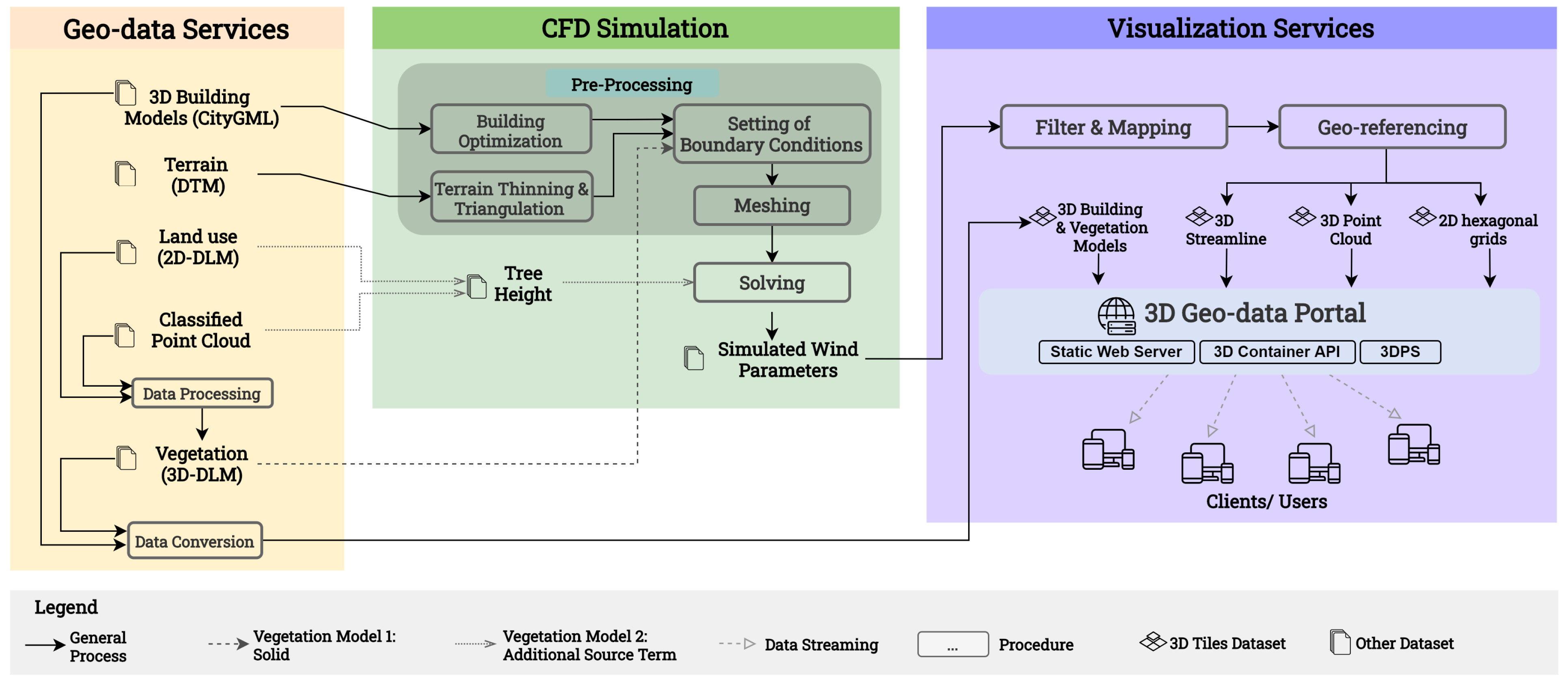
4. Workflow Overview

In this study, a general workflow to interactively explore simulated urban wind fields in a Smart City platform is proposed. This workflow is presented in Figure 1 and consists of the three main parts Geo-data Services, CFD Simulation and Visualization Services.

The Geo-data Services enable access to a multi-purpose 3D city model including 3D buildings (CityGML), a digital terrain model (DTM) as triangulated irregular network (TIN), a 3D digital landscape model (3D-DLM) including vegetation objects, as well as a 2D digital landscape model (DLM) and a classified 3D point cloud. The 3D City model consists of 3D building geometry and other 3D objects while a 3D-DLM is a complete coverage of the environment including roads, land use etc. Both the 3D City model as well as the 3D-DLM can be represented in CityGML. In addition to a model of the built-up area, the Geo-data Services may contain use case specific data about future urban design to support what-if simulations of urban districts as well. The Geo-data Services include a quality management process in the back-end to ensure that only validated 3D city and 3D-DLM models will be provided.

The CFD simulation consists of the application specific preparation of the input data and the simulation itself. As CFD tools usually fail to work with global coordinates, all data are translated to a local coordinate system. The 3D buildings are taken from a valid CityGML, converted and optimized for the CFD simulation using the geometric optimization algorithms that have been developed especially for this purpose [35,36]. The terrain is taken from a DTM. The representation of vegetation objects in this workflow will be investigated using two different approaches. The first approach models vegetation as solid geometric objects taken from the 3D DLM. They are added to the building model before setting the CFD boundary conditions (dashed line in Figure 1). The second approach models vegetation as additional momentum source that is defined directly in the solver of the Navier-Stokes equations. The spatial positions of the sources are taken from the land use classification and the tree height derived from point clouds (dotted line in Figure 1). Having combined all relevant geometric input, the computational domain as well as boundary conditions are defined. In the domain, the computational mesh is generated and the equations are solved on this mesh.

The Visualization Services integrate the 3D building models, the terrain and the simulation results in a web-browser in the 3D Geo-data Portal. For the visualization, the terrain is included from Cesium. In this research, 3D Tiles is used as data delivery format. The simulated wind parameters have to be converted from standard CFD output (CSV files, Comma Separated Values) to 3D Tiles. Only points close to buildings are selected (Filter) and mapped to a suitable color map to sufficiently present the wind parameter details (Mapping). These points have to be translated from the local coordinate system during simulation to the global world coordinate system (Geo-referencing). The three data types, 3D streamlines (e.g., wind flow starting at a specific inlet point), 3D point cloud (e.g., pressure and wind speed at pre-defined positions) and 2D hexagonal grids (e.g., mean pressure value of several points projected on hexagons on the floor and building surface) are provided to the 3D Geo-data Portal. Each client can connect to this 3D Geo-data Portal using only a common web-browser on their end device. This allows the user to interactively explore simulation results without installing any additional software besides a web-browser. It is pointed out that the visualization makes use of the original 3D building model.

With the presented architecture of the overall workflow and its used software, it is not yet possible to control the entire workflow, especially to specify CFD simulations and to automate all geometry optimization steps web-based and directly from the 3D Geo-Data Portal. Because there are still some manual steps necessary, the approach presented in this study is called “semi-automated”.

5. Workflow Details

As the idea and the overview of the general workflow form a basis of understanding, the challenges and solutions of the three main parts of the workflow are considered in this section in detail. Each main part of the workflow has its defined input and output variables. In between lie the detailed workflow challenges as addressed in the sections Geo-data Services Section 5.1, CFD Simulation Section 5.2 and Visualization Services Section 5.3.

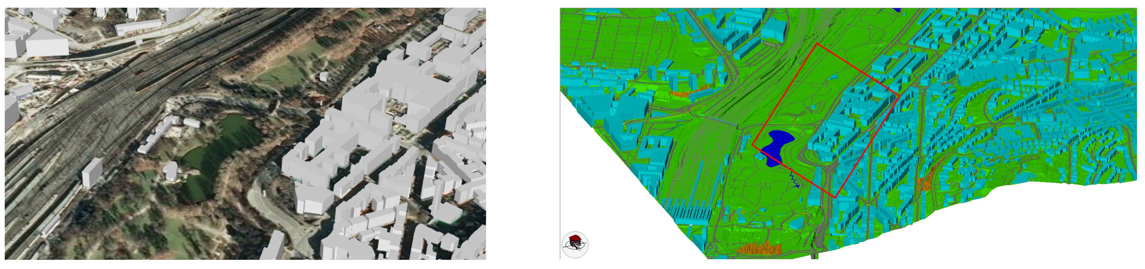
As case study area, a part of the city district Stöckach, known as “Neckartor”, in the city of Stuttgart has been chosen, see Figure 2.

The area that is modeled in detail comprises a busy road with an extensive park on the one side and the selected 75 buildings on the other side, see Figure 2 (left). As the trees and vegetation, which can be seen in the aerial photograph in Figure 2 (right), can have a significant influence on the wind flow, especially since they are present upwind to the domain under investigation, the topography of the terrain and the vegetation has been integrated into the study.

5.1. Geo-Data Services

The entire 3D building model (CityGML) provided by the Stadtmessungsamt Stuttgart consists of about 190,000 buildings in CityGML with LoD 1 (Level of Details). An LoD 2 model is available as well, but was not used in this study. In addition, a digital landscape model of a $2000\mathrm{m}\times 2000\mathrm{m}$ area including the use case area and point cloud data were provided by the Landesamt für Geoinformation und Landentwicklung (LGL). The point cloud includes first- and last pulse-data with a resolution of $8\mathrm{pts}/{\mathrm{m}}^2$. It is classified into point on ground, bridge, building, below ground, and vegetation (including “other non ground points”). The tree cadastre has been provided by the City of Stuttgart.

5.1.1. Implementation

The digital landscape model (DLM) contains linear features such as streets and rivers as well as polygonal features such as residential and industrial areas, forest, etc. The DLM has been tessellated using a FME (Feature Manipulation Engine) workbench [37,38] and extruded to 3D objects based on the point cloud data using the open source software 3dfier [39]. The final DLM was then stored in CityGML [40]. In this process, 3D buildings are modelled as well, but for the proposed workflow they have been replaced by the LoD 1 and LoD 2 building models (CityGML). The resulting 3D-DLM for the city of Stuttgart-Stöckach with 3D buildings and the vegetation is depicted in Figure 2 (right).

Extruded with 3dfier, the geometry of the vegetation objects consists of many small triangles with small angles [41]. It turned out that this model of the vegetation does not match the requirements of the pre-processing of the CFD simulation. Vegetation is thus modeled by a purpose-build FME workbench using both the DLM and some additional data from the tree cadastre to group trees to plant covers with a mean height stored as LoD1 solid geometry in CityGML (for details of the entire vegetation modelling process see [41]).

A lot of research has been done on quality management of 3D city models to ensure the building geometry is consistent and represents the environment within the given tolerance. This research resulted in tools such as CityDoctor [42] and val3dity [43] to validate (i.e., analyse the compliance with the GML-standard) 3D city models. The automated healing of 3D city models, i.e correcting differences according to the standard, is an ongoing research topic.

The CityGML building model as well as the 3D-DLM were validated using the software CityDoctor. The requirements of the CityGML model include a valid solid geometry of every 3D building and plant cover. Typical geometric deficits are duplicated points, non-planar or overlapping polygons, and gaps between neighboring faces. Two points are identified as the same point if their distance is less than 0.1 mm. In contrast to the validation plan recommended in [44], beside a unique identifier of every object, no mandatory attributes are specified. The quality management process was an iterative process with validation of the CityGML model against the requirements and a semi-automated healing process to remove the violations against the specified requirements.

The Geo-data Services consist of the Geo-database management system using the 3D-CityDB with the PostGIS extension [45] (e.g., CityGML, vegetation and land use), a file-based data sharing the specific data itself, as depicted in Figure 1, and the Web Feature Service (WFS) to get access to the data in a web-browser. The data set of the area of interest is specified as a polygonal area and can be accessed from this database using a WFS. Thus, the Geo-data Services provides valid input data for the CFD Simulation and the Visualization Services.

The 3D Geo-data Portal was used to store all prepared 3D datasets to use as an interfaces for clients to access or query the available datasets. At first, this 3D Geo-data Portal was implemented using the static web-server to host all the datasets. To avoid that users had to know the correct end-points and format on the server to access the data, the 3D Geo-data Portal was augmented by the implementation of the data delivery specifications from the OGC: the 3D Container API [46] and the 3DPS [32]. The 3D Container API aims to enable users to browse and query access to the 3D geospatial datasets for streamed data delivery through the nested geospatial volume container resources. The 3DPS is a geospatial 3D content delivery implementation specification standard from OGC specifying the way geospatial 3D contents are described, selected and delivered. Both the 3D container API and the 3DPS were implemented in Node.js with the Express.js framework. Later, these approaches are compared and evaluated (see Section 6) and a suitable specification for different scenarios is recommended (see Section 7).

5.2. CFD Simulation

Within CFD the Navier-Stokes equations are solved numerically on a spatial mesh. The most popular CFD approaches for wind simulations are Large Eddy Simulation (LES) and Reynolds-averaged Navier Stokes simulation (RANS), see [47], where the two approaches are compare in detail: Although LES is able to provide more detailed and more accurate results than RANS, the latter has established itself (not lest because of the lower computing time) and is an adequate choice for many applications such as pedestrian wind comfort, near filed pollutant dispersion and natural ventilation and therefore it is used in this study. The simulations are conducted with ANSYS Fluent as RANS simulation with the k-$\omega$ SST turbulence model [48].

5.2.1. Problem Statement

For wind flow simulations the computational domain is an air filled box with an edge length of several kilometers and height bounded by the buildings and the ground. The domain of interest is only a small part within this box, because large distances to the boundaries are necessary to avoid nonphysical influences on the results. The air volume is subdivided by 3D cells to a so-called mesh. The cells have to have an appropriate size to resolve the physical effects depending on the used CFD approach. They may neither be too small nor too big to avoid nonphysical effects. For the used numerical solvers the computational time depends on grid size, and therefore the grid size also should not be too small to avoid large computational time. Near to the ground and the building surfaces, a so-called boundary layer, consisting of around 5–10 cell layers parallel to the surface, has to be defined with small cell length normal to the surface in order to correctly model boundary effects.

Besides the conversion from CityGML to a CAD data format, there are three important aspects to be considered [35] that mainly apply to the geometry of the buildings:

1.

For meshing, the air filled box should be a “closed” solid and may not contain defects such as gaps in the model, missing or overlapping faces or unclosed geometries such as free faces, edges, and vertices. A few defects can also be repaired by CAD software.

2.

Each geometry edge in the 3D city model is used as basis for cell generation in the 3D mesher for CFD simulations. To resolve the physical effects around a building edge, the cell size has to be even smaller than the smallest edge size in the 3D city model. Furthermore, the smallest edge that will appear in the 3D mesh is a fraction of the smallest edge length in the 3D city model.

3.

The generation of a valid boundary layer can be quite complex or unsolvable for e.g., small gaps between buildings.

Healing of CityGML, as defined in Section 5.1.1, may help to obtain a CAD model after data conversion that largely meets the first aspect, but as pointed out in [23] converting the CityGML to a STL file and then applying a CAD repair tool is unsatisfactory at the moment and still requires (time consuming) manual work. In this paper, the approach of Piepereit at al. [35] is used to modify the geometry for the CFD simulation.

Concerning vegetation, two approaches are used. The first approach uses solids for the vegetation. Within the 3D-DLM the vegetation is modeled as LoD1 solid geometry in CityGML and hence the same requirements apply as for the buildings. Together with the terrain, these plant cover objects and the optimized buildings form the geometric input for the CFD simulation in the first approach (dashed line in Figure 1). Such solid vegetation objects may model the wind shielding effect of vegetation areas, but the effect will probably be too strong. To better model the semipermeable nature of vegetation, a second approach is considered. Within this second approach, the vegetation is modeled as an artificial source term in the Navier-Stokes equations as proposed in [49].

5.2.2. Methodology

As explained in the previous section, building optimization and vegetation modelling are two crucial steps when setting up the model. The CFD simulation is only performed on a selection of buildings due to restricted computing time.

Building Optimization

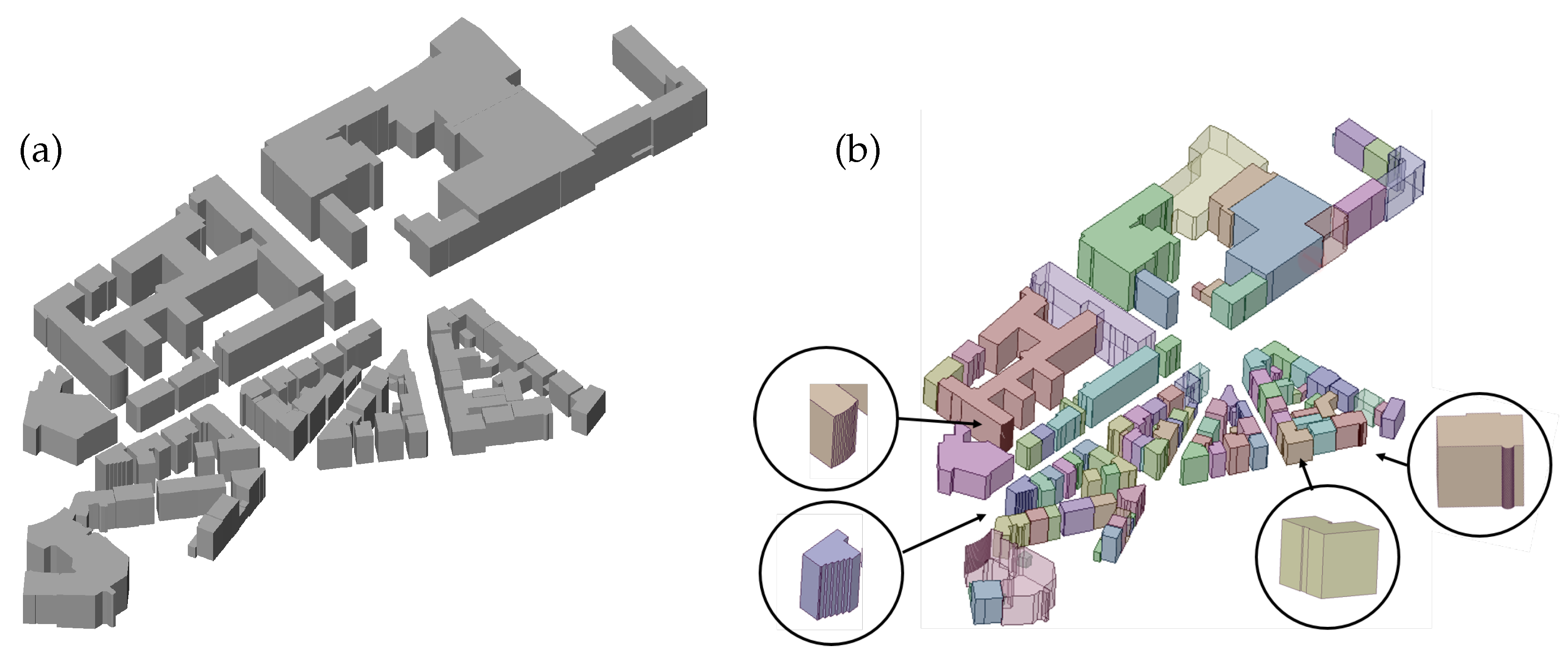
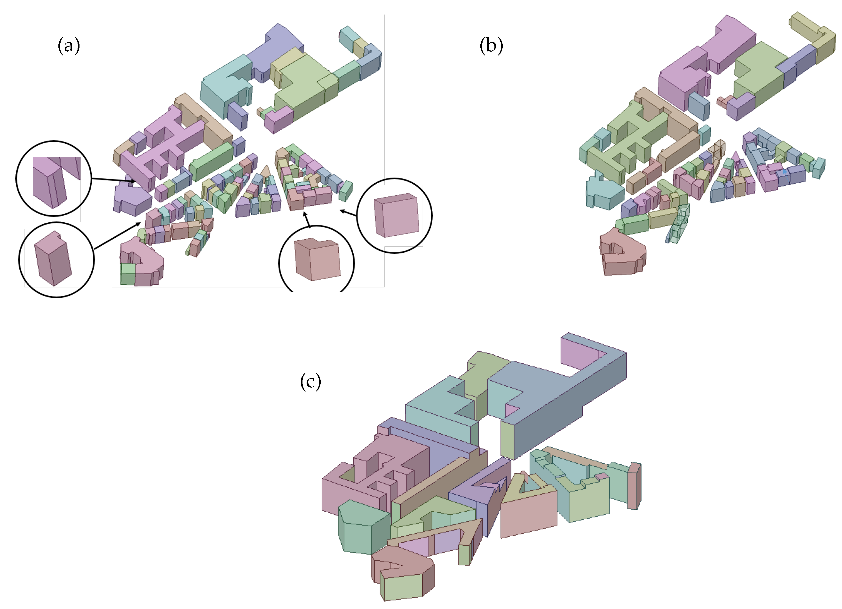
The optimization process starts by using a valid CityGML model of the investigated buildings. Using OpenCASCADE [50], the model can be directly converted to STEP. Figure 3 shows the selected area (a) as CityGML and (b) converted into STEP data format. First, not all buildings can be converted in such a way that they can be further processed by the pre-processing of the CFD tool (the CAD tool ANSYS SpaceClaim in this study) without some manual work. Second, and more importantly with regard to the goal of this work, the building models contain numerous small details which make a mesh generation during the pre-processing for CFD simulations difficult or even impossible.

Therefore, the building model is converted into a CAD BRep data format. After the conversion, edges and faces are merged and a specific sweep plane algorithm is used, as described in [35,36], to simplify the models automatically. During this process surfaces are moved parallel to their normal direction into or out of the building models. Thereby short edges and narrow surfaces are removed iteratively, so that small elements (as they occur in offsets, bulges or corner offsets) are eliminated, which significantly reduces the complexity of the models. To arrive at a reasonable compromise between effort and accuracy in this study, the minimum edge length was set to 2 m. This objective cannot be achieved completely by means of the described automatic processes alone. However, very small edges are removed and the length of the now shortest occurring edge has increased while the number of edges below 2 m is reduced substantially, see

Table 1. Optimization overview. The sweep algorithms increases the smallest edge and substantially reduces the number of small edges. Additional Boolean operations further decrease the number of faces and vertices.

Model	Shortest Edge	# Edges	# Faces	# Vertices	Volume
	[m]	below 2 m			[m${}^3$]
Original	0.014	2172	1715	2874	979,317
Optimized (sweep)	0.098	8	884	1292	971,890
Optimized (sweep and bool)	0.098	8	674	1049	958,240

. This results in a considerable simplification of geometric details, see Figure 4a.

With additional Boolean operations buildings are combined. This also simplifies the model and reduces the number of faces and vertices, see Figure 4b and Table 1. After the automated pre-processing, the building models are converted to STEP and are manually processed further in SpaceClaim. For the mesh generation, some more buildings are combined, gaps between buildings are removed and courtyards are partly closed, see Figure 4c, to enable the boundary layer to be established in the entire simulation domain. Within the whole optimization process, the shape of the geometry is allowed to be changed but the volume of the buildings is kept as close as possible to the original value.

Terrain Model

The terrain can be taken from the existing CityGML TIN elements or from any other elevation data of the area of interest. For the presented use case, a point cloud was thinned and triangulated again with a surface tolerance of 2 m. The resulting STL file of the terrain is imported in SpaceClaim and used as ground surface of the air volume.

Vegetation Models

The implementation of the first vegetation model mentioned in Section 4 is straightforward, as there are only additional solids to be considered in the prepossessing process. The more extensive second vegetation model concerns the height field of the vegetation as well as its location. It is based on the approach of Shaw and Schumann [49] and has been validated using LiDAR measurements for a different site in [15]. It is directly implemented in ANSYS Fluent.

The resistance of the flow passing the vegetation is described by a volume force which is added as a source term to the RANS equations. The additional terms for the x-, y- and z-momentum equations are defined by

$$F_i=\rho c_{d}a\left(z\right)\left|u\right|u_i,$$

(1)

where $\rho$ is the density and $c_d=0.15$ the drag coefficient. The variable $\left|u\right|$ describes the velocity magnitude and $u_i,i=1,\dots ,3$ the velocity component in i-direction. The height depending parameter $a\left(z\right)$ represents the resistance induced by the leaf density of the vegetation. The profile of the leaf area density $a\left(z\right)$ is known from the literature [49]. The Leaf Area Index (LAI) describes the tree density and is the integration of $a\left(z\right)$ over the height h. The profile of the leaf area density is described by Shaw und Schumann [49]. For winter a LAI of 0.5 is taken and for summer a LAI of 3.5, based on the work of Bequet et al. [51]. With different leaf density profiles and LAI values, every type of vegetation can be modelled in the simulation.

The coordinates of the investigated area are exported from OSM and transferred to the model. The local height of the vegetation is obtained and calculated from the classified 3D point cloud provided by the Geo-data Services. The point cloud is divided into ground and vegetation marks and contains $10\mathrm{m}\times 10\mathrm{m}$ tiles for the vegetation zone. The vegetation height is calculated by the difference of the vegetation and ground marks and determined per tile. These vegetation heights are shown in Figure 5.

Complete Model, Boundary Conditions

The computational domain has to be rather big to allow the air flow to develop before it hits the buildings under investigation and to avoid non-physical influences from the boundary conditions. According to best practise guidelines [12], the size of the computational domain has to be chosen depending on the height $H_{\max }$ of the highest building in the considered built-up area. With $H_{\max }=31.3\mathrm{m}$, a domain size of $2270\mathrm{m}\times 2000\mathrm{m}\times 1200\mathrm{m}$ has been chosen for this study. This is even larger than recommended in [12] to reproduce the valley meaningful. The domain of interest is placed in the middle of the computational domain and modelled in detail, see Figure 5.

The built-up area is located in a valley with an altitude difference of 150 m. Thus, the topography is considered in the CFD simulations. Upstream of the built-up area a green area with high trees is located. The green area in the center of the investigated area is modelled with the different approaches which are described above. Buildings and vegetation offsite are modelled by a surface roughness value of $0.75$.

The inflow direction is 210${}^{\circ }$ on a 360${}^{\circ }$ wind rose, which is the main local wind direction. For the velocity inflow boundary condition a potential law is chosen

$$u\left(z\right)={\left(\frac{z}{z_{\mathrm{ref}}}\right)}^{\alpha }{u}_{\mathrm{ref}}$$

(2)

with a reference velocity $u_{\mathrm{ref}}$ = 2.5 m/s at a height of $z_{\mathrm{ref}}=10\mathrm{m}$. The exponent is $\alpha =0.28$ according to the urban areas with high and irregular buildings. The terrain and the buildings are modelled as a solid wall with zero velocity at the walls, for the outlet a pressure-outlet boundary condition is chosen. The other surfaces are modelled by a zero-gradient boundary condition. The model must be rotated for each wind direction, so that that the inflow plane is perpendicular to the inflow direction. In Figure 5 the inflow is from the left.

The size of the grid cells varies from small cells in the vicinity of the building to larger cells in the free regions near the boundaries. Here, the 3D mesh consists of around 1.5 million tetrahedral cells, whose edge length range from 0.7 m in the boundary layers over 6 m in the vegetation zone to 40 m in the free regions.

The RANS simulations were performed on 16 CPUs on the bwUniCluster (Intel Xeon Gold 6230). The computation time was 48 h for the case without vegetation and with the additional volume force model for vegetation. With the solid vegetation model (see Section 4) it takes 53 h as there are to more cells in the mesh to resolve the surface of these additional solids with the boundary layer.

5.2.3. CFD Results

The simulation has been performed with the different vegetation models, which differ in accuracy and model depth.

Four cases have been simulated: without any vegetation, with the vegetation modelled as a solid body and with vegetation modelled as a volume force with summer and winter foliation.

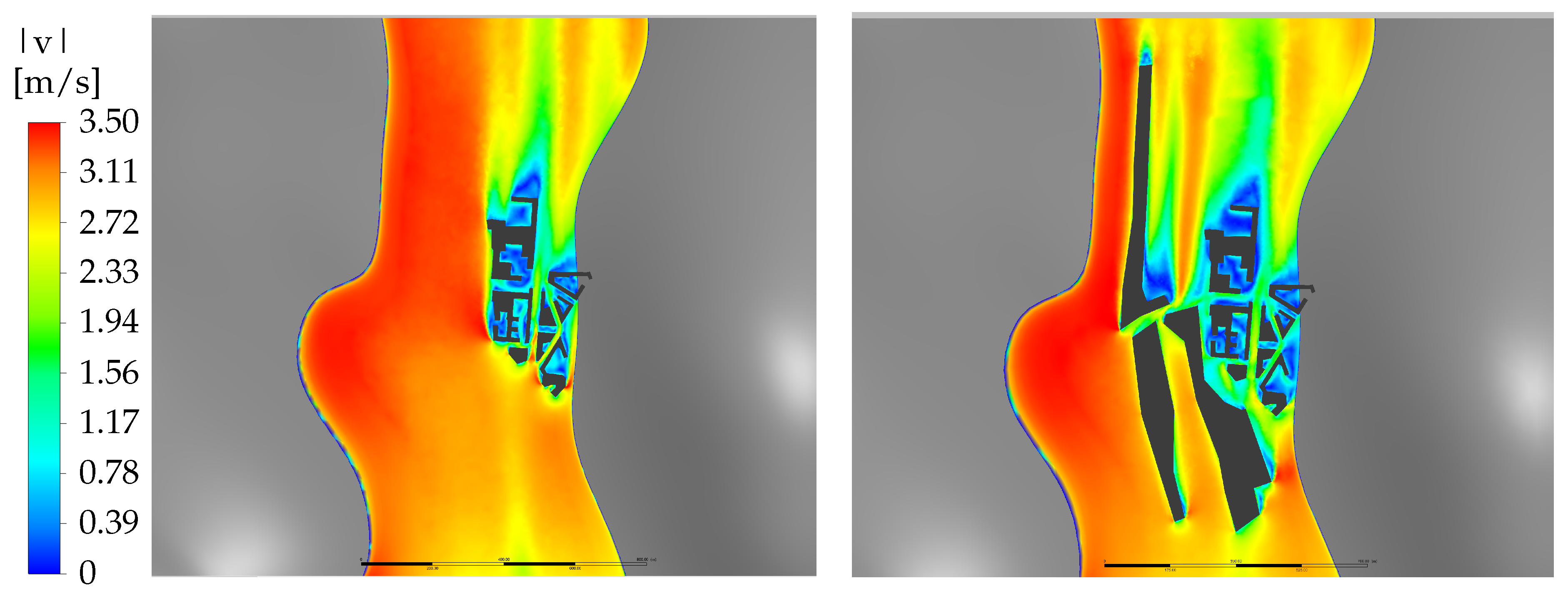
The case without any consideration of vegetation zones, see Figure 6 (left), was used as reference. In the figures the magnitude of the simulated wind speed is shown. The evaluation height is close to the building height, so the grey zones besides the evaluation plane are due to the valley shaped topography. Within the built-up area the flow is considerably decelerated compared to inflow velocity. It should be noted that an evaluation away from the detailed modelled area would be less accurate and may not represent the real flow field.

Figure 6 (right) shows the simulation results with the vegetation modelled as a solid bodies. The results clearly show the local changes of the velocity field in the vicinity of buildings, especially deceleration zones, where the vegetation is in front of the built-up area. Compared to the simulation without vegetation, the wind speed is much lower on the left border of the buildings.

Figure 7 shows results with the vegetation modelled as a volume force in summer (left) and in winter (right). Compared to the first vegetation using solid bodies, in this second model the vegetation zone is meshed. Thus, the flow within the trees is simulated and the vegetation is not explicitly visible in Figure 7. The influence of locally clustered trees can be observed in the velocity field. The flow within the built-up area is significantly lower compared to the solid body vegetation simulation. The comparison between summer and winter shows the noticeably higher velocities in vegetation zones during winter. The lower foliation of the trees leads to lower resistance within the vegetation model and consequently to higher wind speeds. Within the built-up area the change of the velocity diminishes with more distance to the vegetation and the building geometry is starting to dominate the flow.

5.3. Visualization Services

5.3.1. Problem Statement

Visualization of CFD results in post-processing tools of CFD software packages is a common method to quickly interpret and understand the results or at least obtain an intuition about the validity of the simulation. It is imperative that CFD simulation results are condensed into an understandable level of detail to make them available to large number of usersl—who for the most part have no background in CFD data analysis. To enable general users the exploration of CFD results in a common web-browser is another challenge because it involves simplification, abstraction, conversion and delivery of data (formats) through defined protocols.

5.3.2. Methodology and Implementation

The process to prepare the CFD results for interactive visualizations in the web was based on the work presented in Schneider et al. [52] and is summarized in this section. The numerical wind field data obtained from the CFD simulations using ANSYS Fluent were delivered as CSV files. Because CFD is performed on a much larger air volume than the actual object of interest contains in order to avoid artifacts caused by the boundary effects, data points which were higher than twice the building height were removed (filtered). This lead to a greatly reduced number of points and thus to a smaller file size and clearer visualizations later on. After the filtering, data stored in the local coordinate system of ANSYS Fluent were geo-referenced in the EPSG:31467 coordinate system as the reference, i.e., the buildings (in the original CityGML) was stored in this coordinate system. Thereafter, all points were converted to EPSG:4326 also known as WGS84 using the NTv2 (National Transformation version 2) algorithm. The WGS84 is the destination coordinate system which is one of the formats that the Cesium viewer used for the client supports. Cesium was also used to provide the terrain model using a Cesium asset “world Terrain” with an approximate resolution of 30 m [53]. The wind pressure and velocity data were scaled to fit within three 8-bits unsigned integers to encode the color of the information into RGB values for use in the visualization. This part of the color mapping processes is the basis for the color viewed in the visualization of the results.

To allow data delivery through web-services, the post-processed wind data were stored in web-enabled bounding volume hierarchy data formats, including 3D Tiles [54] and geoJSON. The former allowed streaming and hierarchical data fetching in order to deliver and visualize large data sets swiftly to the client and render data efficiently. The latter format was used mainly for investigating and comparing loading times, rendering performance and subjective evaluation of the user experience using different visualization schemes because it provides simple ways to implement stylistic options such as clamping to the ground.

Visualization schemes of the wind data set were implemented as 3D point clouds (pressure and wind components, Figure 8), 2D hexagonal grids overlaid on top of the 3D building models (Figure 9a) and 3D streamlines as point clouds and as Cesium native polylines (Figure 9b,c, respectively). The point cloud data (Figure 8a) was summarized using hexagonal bins using a certain width (5 and 15 m). To perform the hex-binning and create the hex-grid, the Whitebox GAT [55,56] software packages was used. The software is an open access and allows the user to modify the source code of every single algorithm within the package. This option was used by extending the functionality of the binning algorithm to include an averaging of the pressure values within the CFD data set. Thus each cell in the resulting hex-grid represents the average pressure value at a certain height within a specified area.

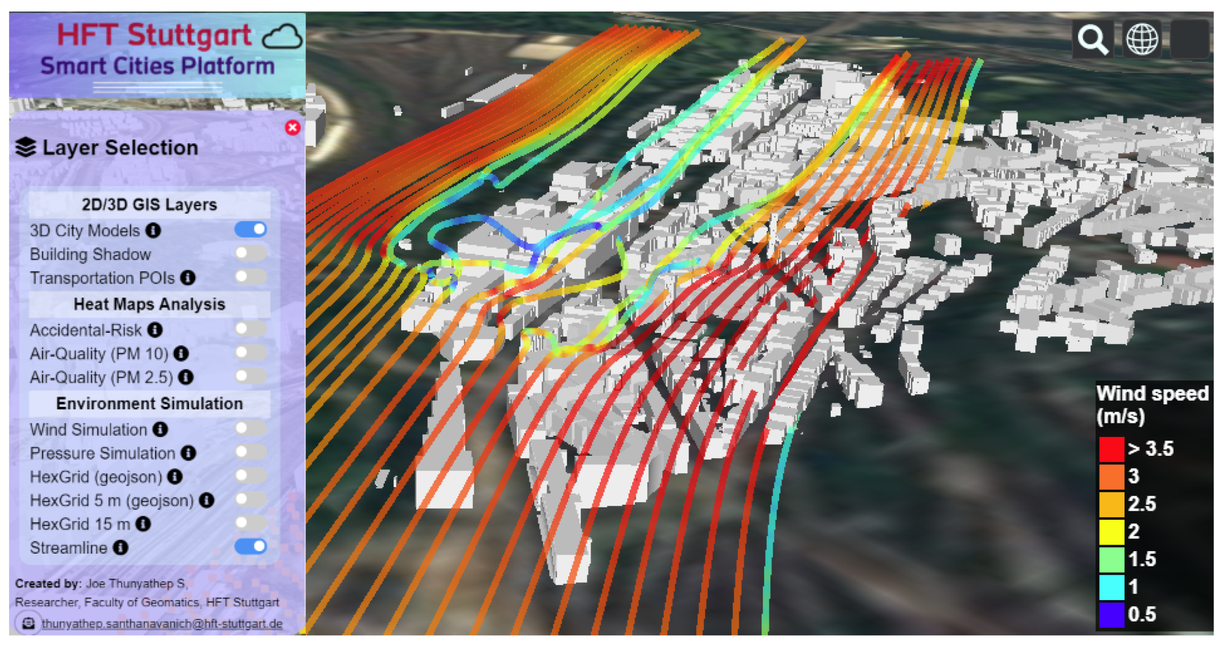
For the visualization of streamlines, Cesium native polylines were employed for which the colorsPerVertex attribute was enabled. This generated a continuous streamline comprised of multiple segments where for each segment a specific colored (according to the mapping of wind speed to RGB) was assigned. Interpolation between vertices lead to a smooth transition between wind speed values, i.e., colors (Figure 9c). The 3DPS API was used to deliver the streamline data (i.e., a list of coordinates and wind speeds as well as corresponding RGB values) to the client. The streamlines can then be generated by the client using simple browser JavaSript within the displayed web site. For visualization of streamlines as point clouds, the same method as described for the point cloud pressure schemes (above) applies because it is the same data format and thus can also be delivered as a point cloud layer using the 3DPS API.

The 3D CityGML building models and 3D-DLM were converted to the 3D-Tiles format using FME. The visualization services use the 3D Geodata-Portal (Section 5.1) as an interface for web-clients to access the data contents.

6. Results and Evaluation

6.1. 3D Geo-Data Portal

The 3D Geo-data Portal was implemented with different approaches, including the static web server, 3D Container API and 3DPS. Several metrics are used for comparing these three approaches, see

Table 2. Comparison of different approaches for the 3D data management in the 3D Geodata-Portal.

	Static Web Server	3D Container API	3DPS
Implementing difficulty	simple	moderate	difficult
Server requirement	low	low/moderate	high
Spatial filter	no	support (2D, 3D)	support (2D)
Spatial query	no	no	support (2D)
Hierarchical geometry structure	no	yes	no
OGC API conformance	no	yes	no

. For the static web server, it is simple to implement but it lacks important server-side operations which provide more flexibility to request data. The 3D container API is more advanced, providing the server operation for spatial filtering in both 2D and 3D and conforming with the OGC API. It also has a hierarchical geometry structure that allows users to access each data layer according to geographic levels; for example, Europe -> Germany -> Stuttgart. Lastly, the 3DPS is the most difficult to implement but provides spatial querying allowing users to query and extract the dataset in the specified spatial boundary.

6.2. CFD Simulation

At the beginning of the project, all components of the model (buildings, terrain, vegetation) had to be converted manually from GIS databases and optimized and combined manually for CFD simulations. The developed semi-automated workflow significantly reduces the manual effort in the main time-consuming steps, see

Table 3. Comparison of manual and semi-automated workflow for the case study with 75 buildings.

	Manual	Semi-Automated
preparation + optimization	1 week	1 day
of buildings for CFD
vegetation	few minutes	1 h
	(inaccurate)	(accurate)
terrain	few minutes	few minutes

.

The most time-consuming part is the preparation and optimization of the buildings. The manual optimization of the selected 75 buildings needed around a week after conversion of the geometry. With the newly developed sweep-plane-algorithm (see Section 5.2.2) the optimization of these buildings takes about a day. By simplifying the geometry of the buildings as described, the quality of the derived computational mesh can be significantly improved.

The vegetation models (see Section 5.2.2) differ in accuracy and model depth and can be applied in around an hour within the proposed workflow. The vegetation model with additional source terms can easily be integrated. It additionally leads to a even more realistic wind field and is suggested for further simulation cases.

The rotation and cutting of CFD domain to make it consistent with the inflow wind direction as well as the definition of e.g., edge parameters and boundary layers for the mesh generation has still to do be done manually.

6.3. Visualization

The implemented visualization pipeline, including data pre-processing, filtering, mapping and conversion requires many supervised and elaborate steps using various software packages (such as GIS software, Matlab and Python scripts). Once data has been transformed into the appropriate formats, JavaScript is used to implement the front-end visualization platform. The resulting Smart City Platform can be seen in Figure 10, where the user has several options to obtain different kind of data representations of the CFD results, as well as request additional data such as 3D building models. These requests, which happen by a simple click are handled using the implementation of the 3D Geo-data Portal (Section 6.1). As the 3D Geo-Portal uses the original building model converted to 3D Tiles, the buildings presented in the 3D Geo-data Portal slightly differ from the optimised buildings used in the CFD simulation, sometimes leading to visual artifacts as intersection of streamlines with buildings.

As different data formats for the web-application have been tested a recommendation can be made as to which format is best suited for the purpose of visualizing large geo-spatial dataset (

Table 4. Average loading times (out of 10 iterations), measured using Google Chrome Developer Tools. Table extended from [52].

Layer (Data Format)	Resource Sizes	Loading Time	Subjective Experience
Point clouds (3D Tiles)	2.77 MB	550 ms	loading is very fast, instant interaction possible, fast rendering
Hex-grid (3D Tiles)	1.45 MB	673 ms	fast loading times and rendering, instant interaction possible
Hex-grid (geoJSON)	3.07 MB	952 ms	low loading, application unresponsive for several seconds, slow rendering
Streamlines (3D Tiles)	1.05 MB	452 ms	same as Hex-grid (3D Tiles)
Streamlines (Cesium)	0.2 MB	152 ms	loading and rendering is fast, slight lag noticeable until full responsiveness

). However, this finding may not just be limited to our CFD results but may extend to similar data based on entirely different physical measurements or simulations. As can be seen from these results, 3D Tiles (or other bounding volume hierarchy formats) are best suited for the purpose of a smooth and fast loading web-application when dealing with spatially spread out and fine granular data.

7. Discussion

The goal of this study is to enable the integration of offline CFD simulation results in a Smart City platform. In general, the proof-of-concept for the proposed workflow was executed successfully. It provides a faster setup for CFD simulations from a geo-informatics data basis and allows CFD results to be easily accessible in interactive web-based applications.

The workflow to setup the CFD simulation (presented in Section 5.2), results in a simplified and well conditioned building geometry. This is a prerequsite for high-quality and appropriate meshing which has a large impact on the outcome of CFD simulation [21]. However, the term appropriate is highly dependent on the research question at hand and scale of the model. A significant time saving of around 85 % for building optimization (Table 3) using the pre-processing algorithms of [35] was observed compared to the fully manual process. Despite this huge improvement, some manual interventions may be needed for complex geometries, before meshing becomes possible. Because of this, further development of the geometry optimization algorithm is of future interest in order to implement additional simplification steps for specific urban wind issues such as closing of gaps between buildings and courtyards. Due to the presented semi-automated workflow, faster model pre-processing and preparation of results for various CFD applications are feasible.

Although simplification/optimization, which modifies the geometry, is in some way or another performed in all CFD studies, up to now the influence of modifications has been systematically studied only by [57]. The impact on the CFD results caused by the modifications proposed in the present study remains to be examined systematically for every specific application.

With respect to the visualization and presentation of results in an explorable web-based application, the 3D Geo-data Portal was used to deliver the 3D city models and 3D wind simulation data sets. The 3D Geo-data Portal supports mobile devices without any further implementation and simplifies the visualization outdoors. The main challenge is the streaming of the 3D data sets from the visualization server to the client. Storing wind or pressure representations in different data formats (e.g., 3D Tiles and geoJSON) exhibits a noticeable difference in response time (i.e., 3D Tiles loads 30% faster than geoJSON), the subjective experience is even more noticeable (Table 4). Although a static web-server implementation would have been the easiest solution, it is also the one with the least flexibility concerning data delivery and accessibility. Thus, the experimental 3D container API specified in an OGC pilot [46] and 3DPS OGC standard were implemented to allow query and data access via the respective APIs (Table 2). The 3D Container API, provides an easy-to-use interface for users to browse through the hierarchical geometric levels for obtaining the data set end-points. This provides benefits to new users to understand the service quickly but it is difficult to add more scenarios or update existing data. 3DPS supports spatial queries for data in specified geometric boundaries. Thus, the 3D Container API is recommended for data delivery service to share data broadly and to integrate in any simple applications, while 3DPS is recommended to be used in more complex applications that provide various scenarios. To the authors’ knowledge, this is the first study that has used 3DPS and the 3D Container APIs to deliver CFD simulation data into a 3D explorable web-application for visualizing urban wind fields at the scale of buildings and below. For the visualization of continuous streamlines the 3DPS API was used to deliver the distinct simulation data format (i.e., coordinates, wind speeds and color values). This way to deliver wind simulation results (i.e., streamlines) to web clients has not been done before and highlights the flexibility of 3DPS, although the API was not specifically designed to deliver such data. In fact, 3DPS does not specify the type of data that should be delivered, thus allowing for great flexibility within a server-client-data relationship.

In the presented case study, the existing buildings are taken into account. The same methodology can be applied to new urban designs, integrating the planning stage of new buildings in the 3D city model. This would allow architects and urban planners to analyse several possible designs with respect to urban wind flow and its implications. However, in the web-service, it is not yet possible to run CFD simulations interactively as it is in the Kalasatama Digital Twins Project [25]; furthermore, it is not possible to change building geometry on-the-fly within the web-application. In the presented solution, alternative building models have to be provided in the Geo-data Services and CFD simulations with new buildings and/or different boundary conditions such as different inflow conditions have to be provided in advance. This is because the pre-processing for the CFD simulation still requires expert knowledge as well as manual work and the CFD simulation itself is time consuming and requires adequate computational resources. This may be considered to be a limitation on one hand, but on the other hand, this procedure helps to ensure the quality of the CFD results, which depends on the quality of the mesh which in turn depends on the geometry features. Furthermore, compared to the approach in [25] it is not required that those users, who finally examine the results such as urban planners, have access to the CFD software. Finally, the architecture proposed in the present paper is open to the integration of any CFD software that allows data export, and beyond that any simulations software that provides similar data.

8. Conclusions

This paper investigated and presented, for the first time, a continuous workflow from 3D city models to the visualization of simulated wind fields in an urban environment. This continuous workflow employs a new pre-processing workflow, using newly developed algorithms to simplify building geometry [35,36], that semi-automatically enables an optimization of building geometry to perform more efficient CFD simulations in terms of ❶ substantial time savings for manual labor, and leading to improved computational efficiency and simulation convergence. Additionally, ❷ data delivery for these specific CFD results from a server to an interactive web-based client was implemented using state of the art OGC standard protocols for the first time. Using these standard protocols, specifically the 3DPS API, a new approach for the streamline delivery from server to client was developed exploiting the fact that the 3DPS protocol is highly flexible due to its intentional lack of specificity for data delivery formats. Finally, the presented workflow concludes with ❸ implementation and analysis of different visualization schemes of urban wind fields with respect response time and user experience ❹ within the context and at the scale (and below) of 3D building models. Ultimately, ❺ the presented collective of novel interdisciplinary solutions for a variety of specific problems at the interface between CFD and geoinformatics (see Section 5) has not been presented before, to the knowledge of the authors. ❻ While this workflow is applied within the Smart City context in this study, it furthermore may serve as (an almost) step-by-step guide for other domains, dealing with the same or at least similar issues, e.g., flood simulation.

Notwithstanding, more research is needed with respect to the parameter-based geometry optimization algorithm for the CFD setup, as a manual pre-processing step is still required afterwards, thus limiting the number of buildings that can be examined.