A Three-Dimensional Visualization Framework for Underground Geohazard Recognition on Urban Road-Facing GPR Data


Abstract
:1. Introduction
- (1)
- We presented a framework that integrates the detection processes into one workflow, including data acquisition, preprocessing, modeling, visualization and interactive geohazard recognition and analysis. The data acquisition is based on the self-developed GPR equipment. Data formats and the loosely coupled formats make the framework load data in a flexible way. The details are described in Section 3.1.
- (2)
- In this framework, a series of proposed novel algorithms provided the theoretical support for the recognition processes, including the data selection methods of the Kriging algorithm, the improved GPU-PSO-Kriging algorithm and the layer-constrained triangulated irregular network (TIN) algorithm. These can not only make the GPR data preprocessing faster and more accurate, but can also construct geohazard bodies of arbitrary shapes either in part or as a whole. A detailed description of this framework is formulated in Section 3.2, Section 3.3, Section 3.4 and the visualization results are described in Section 4.
- (3)
- In this work, we did not only provide a theoretical analysis and experimental verification for the framework with related algorithms, but also developed a platform system to test the effectiveness of the proposed framework and its algorithms in a practical dimension.
2. Existing Works
2.1. GPR Data Acquisition
2.2. GPR Data Preprocessing
2.3. 3D Geological Modeling
3. The Principle of 3DVF4UDR
3.1. Overall Description of 3DVF4UDR
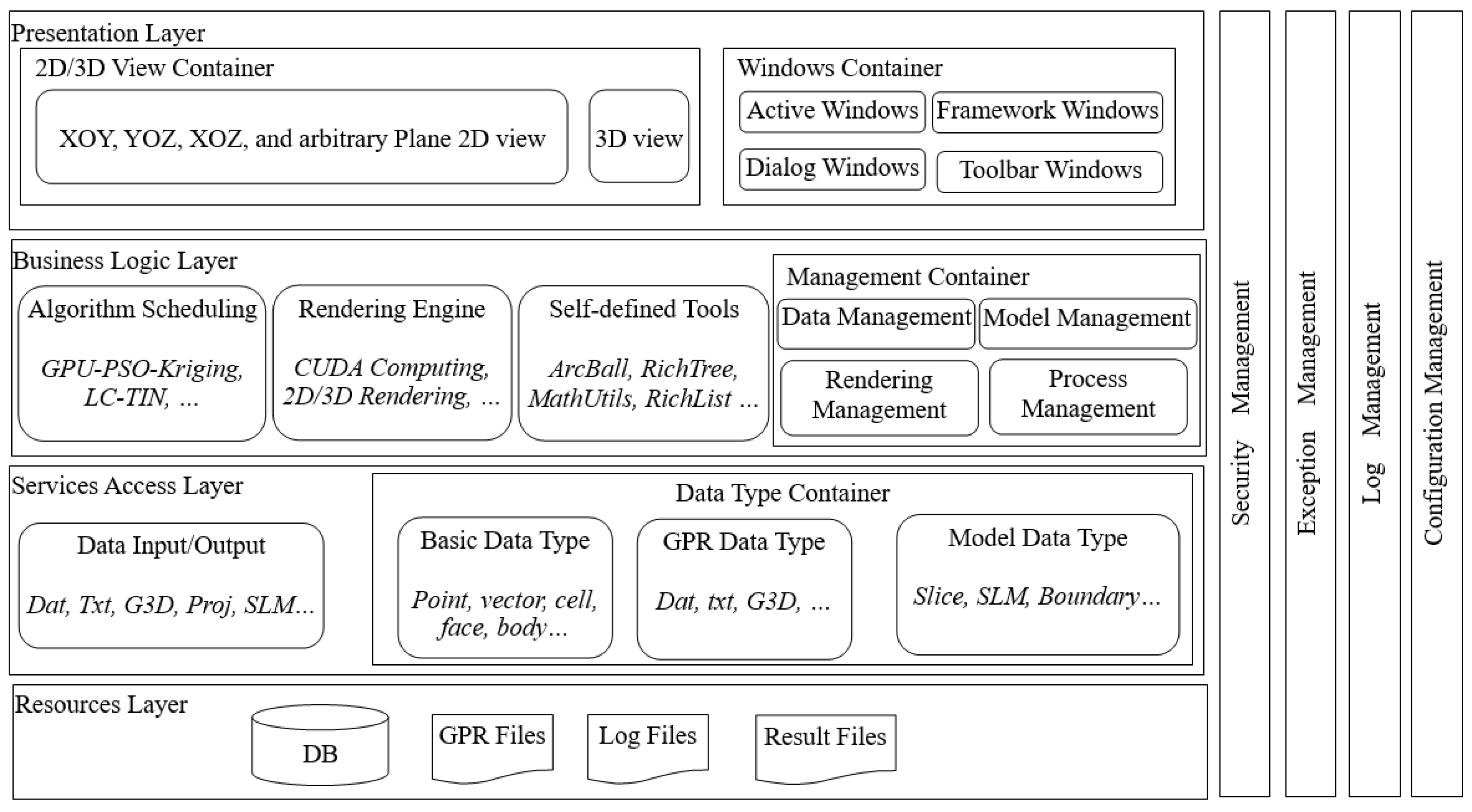
3.1.1. The Architecture
3.1.2. Workflow Description
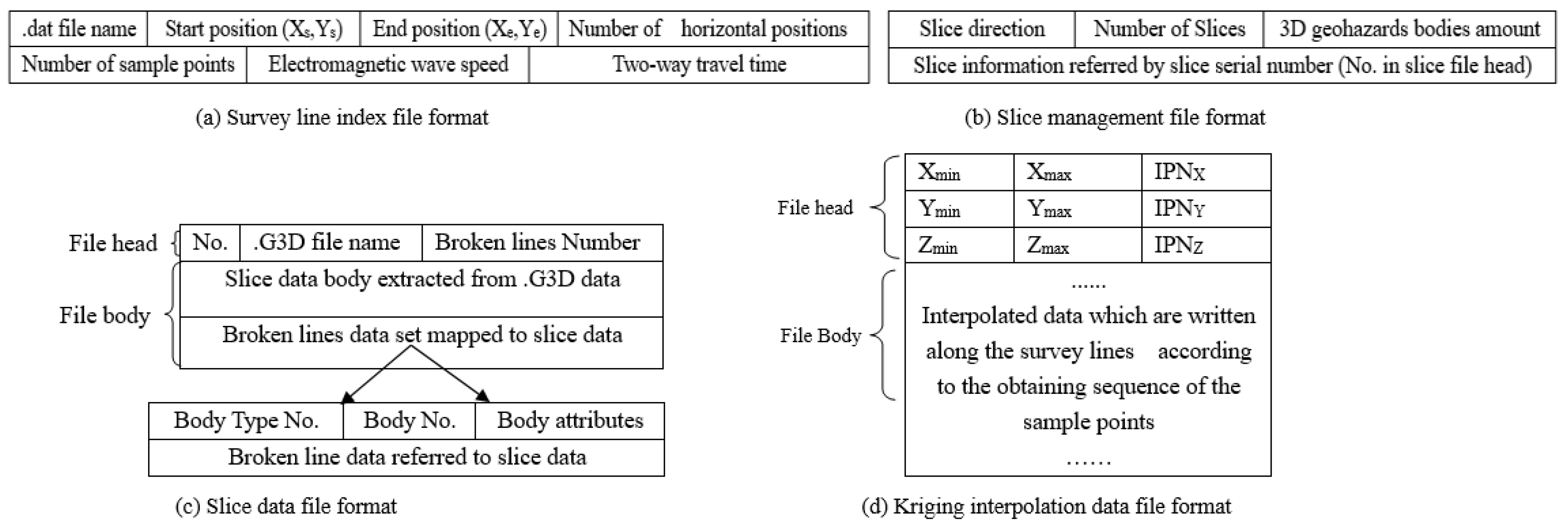
3.1.3. File Format Descriptions
3.2. Data Preprocessing
3.2.1. Sampling Point Selection Algorithms
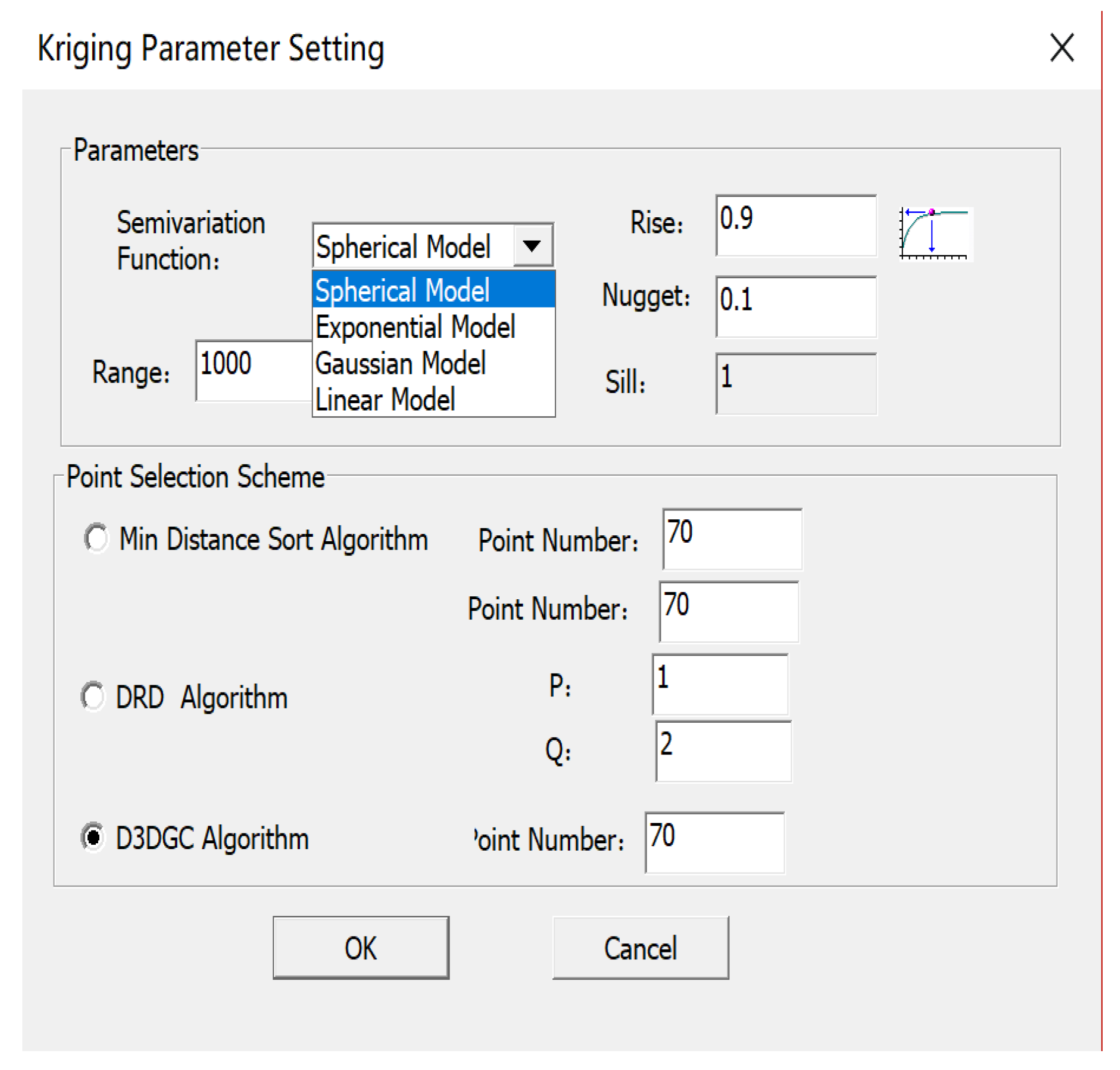
3.2.2. GPU-PSO-Kriging Algorithm
| Algorithm 1 The Steps of the GPU-PSO-Kriging Algorithm |
| Input: , c1, c2,, Output: c, , a Steps
|
3.3. Data Modeling
| Algorithm 2 The Steps of the LC-TIN Algorithm |
| Input: Output: Ω Steps
|
3.4. Data Analysis
| Algorithms 3 The Steps for Computing a Geohazard Body |
Steps
|
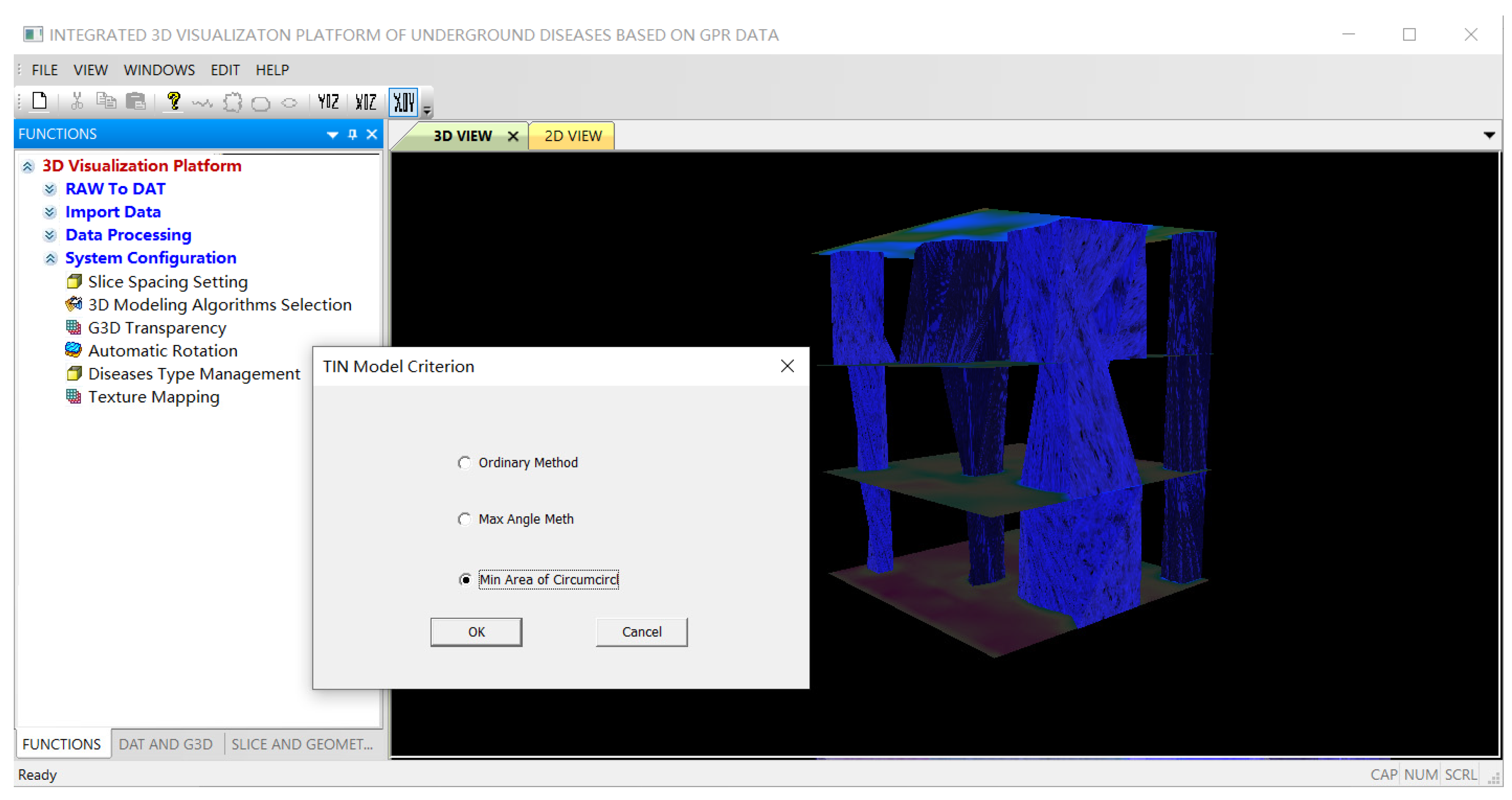
4. The Application of 3DVF4UDR
4.1. Experimental Environment and Data
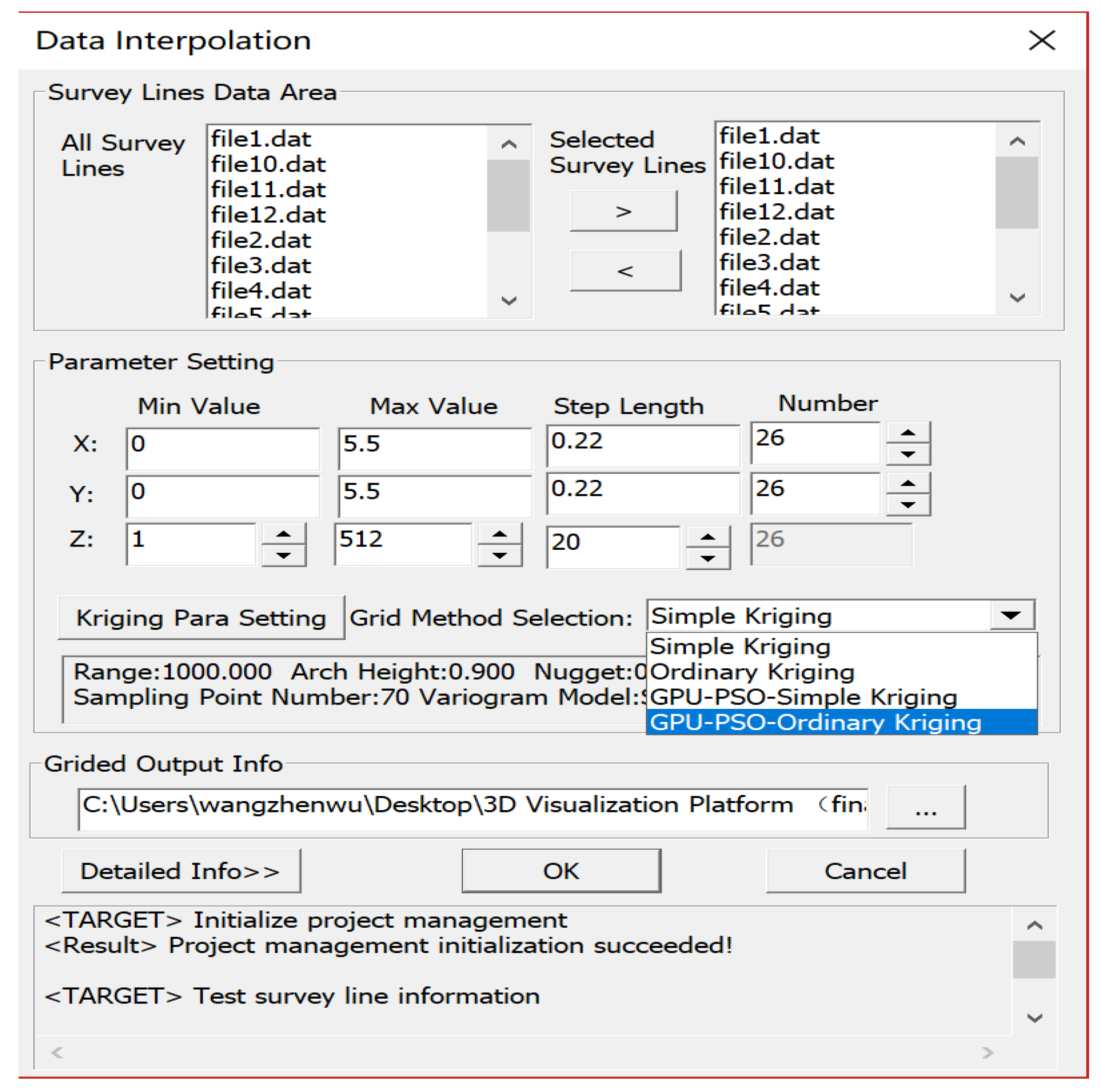
4.2. Data Preprocessing
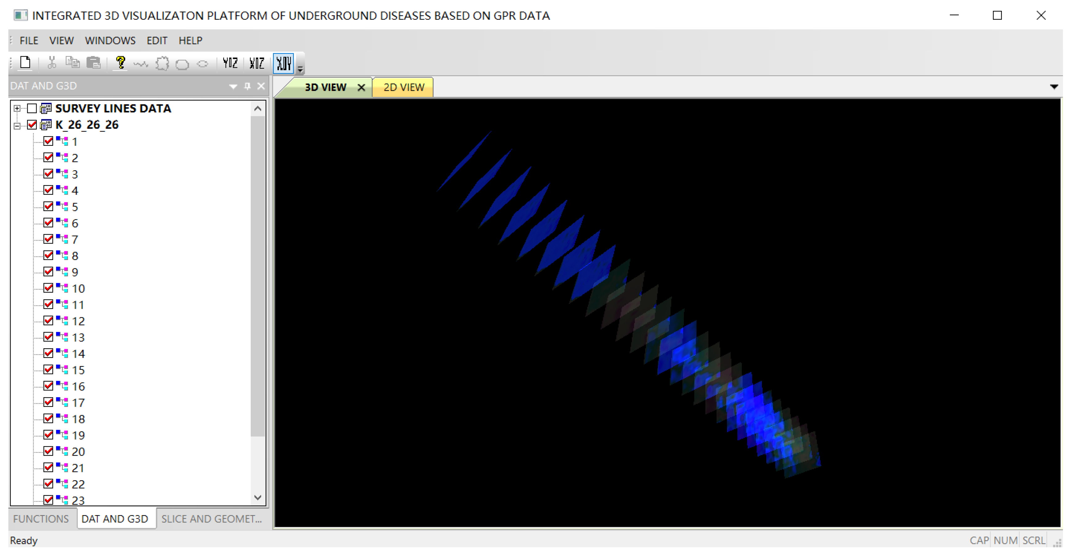
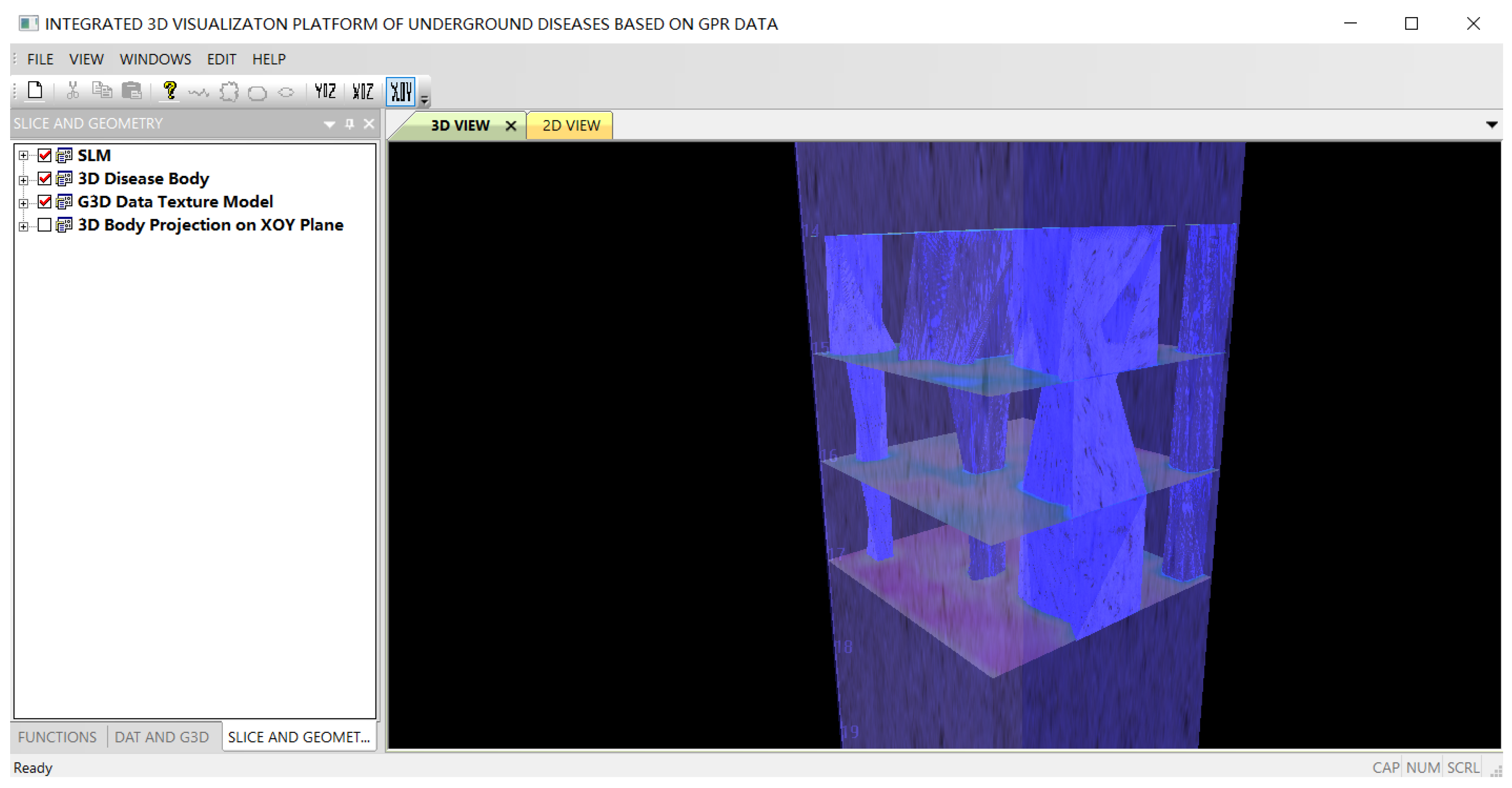
4.3. Data Modeling
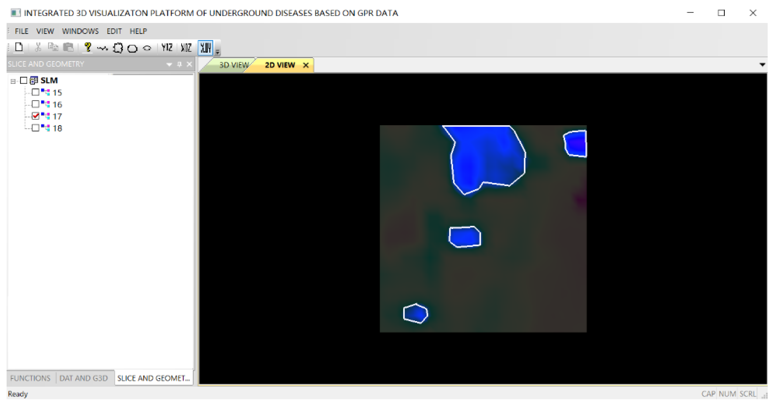
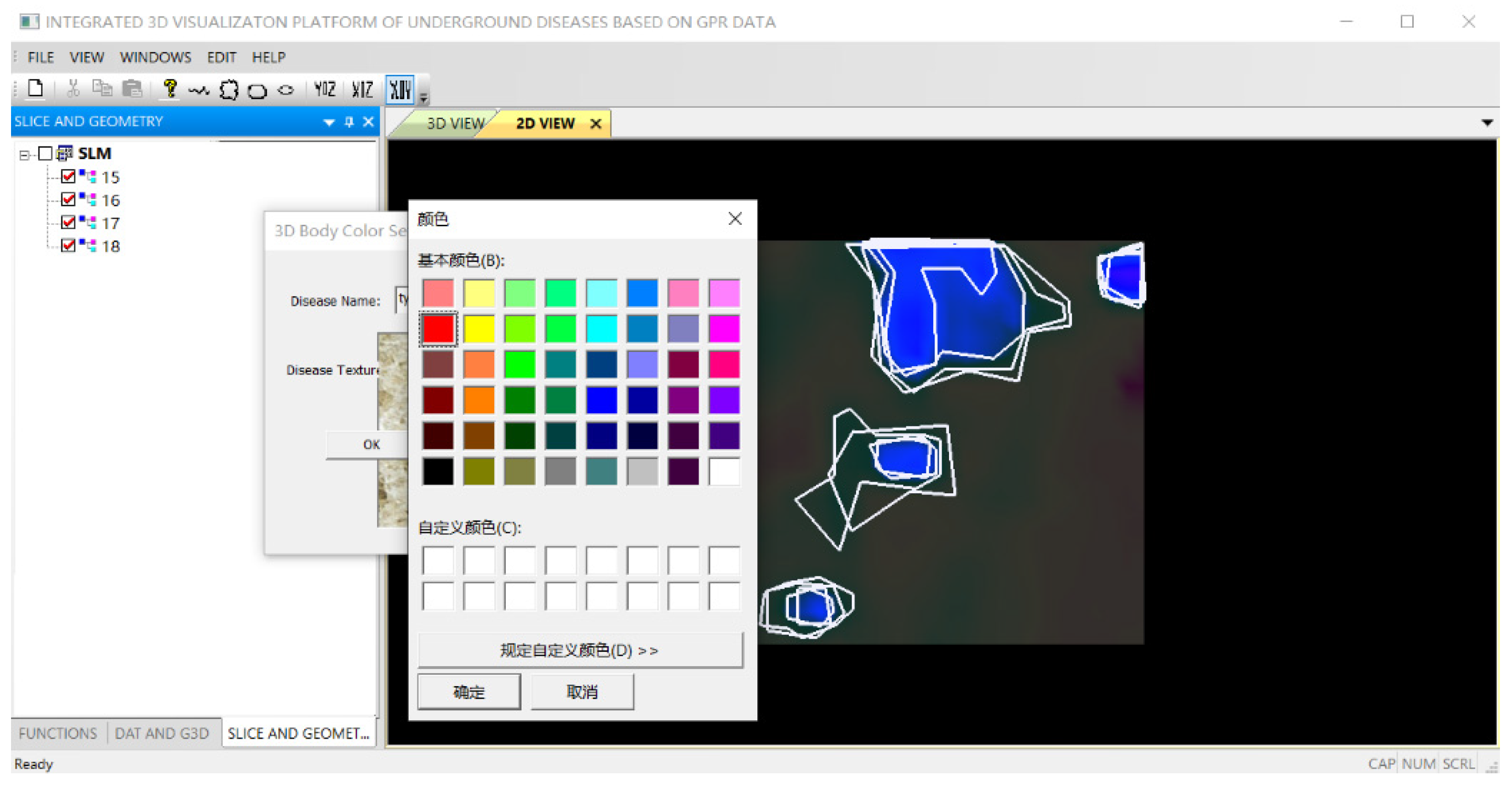
4.4. Data Analysis
5. Conclusions and Future Work
Author Contributions
Funding
Conflicts of Interest
References
- Hadimlioglu, I.A.; King, S.A.; Starek, M.J. FloodSim: Flood Simulation and Visualization Framework Using Position-Based Fluids. ISPRS Int. J. Geo. Inf. 2020, 9, 163. [Google Scholar] [CrossRef] [Green Version]
- Wielebski, Ł.; Medyńska-Gulij, B.; Łukasz, H.; Dickmann, F. Time, Spatial, and Descriptive Features of Pedestrian Tracks on Set of Visualizations. ISPRS Int. J. Geo. Inf. 2020, 9, 348. [Google Scholar] [CrossRef]
- Dalyot, S.; Doytsher, Y. Multi-Temporal Time-Dependent Terrain Visualization through Localized Spatial Correspondence Parameterization. ISPRS Int. J. Geo. Inf. 2013, 2, 456–479. [Google Scholar] [CrossRef] [Green Version]
- Lathrop, R.; Auermuller, L.; Trimble, J.; Bognar, J. The Application of WebGIS Tools for Visualizing Coastal Flooding Vulnerability and Planning for Resiliency: The New Jersey Experience. ISPRS Int. J. Geo. Inf. 2014, 3, 408–429. [Google Scholar] [CrossRef]
- Wang, W.; Hu, C.; Chen, N.; Xiao, C.; Jia, S. Spatio-Temporal Risk Assessment Process Modeling for Urban Hazard Events in Sensor Web Environment. ISPRS Int. J. Geo. Inf. 2016, 5, 203. [Google Scholar] [CrossRef] [Green Version]
- Hu, Y.H.; Bai, Y.C.; Xu, H.J. Analysis of Reasons for Urban Road Collapse and Prevention and Control Countermeasures in Recent Decade of China. Highway 2016, 61, 130–135. [Google Scholar]
- Seong, J.-H.; Jung, M.-H. Determination of priorities for management to reduce collapse accident of open excavation and road sink in urban areas. J. Korean Tunn. Undergr. Space Assoc. 2017, 19, 489–501. [Google Scholar] [CrossRef]
- Cong, W.; Mao, P.; Zhuang, L. Application of 3D GIS in urban underground space planning. Chin. J. Geotech. Eng. 2009, 31, 789–792. [Google Scholar]
- Evans, R.; Frost, M.; Stonecliffe-Jones, M.; Dixon, N. Ground-penetrating radar investigations for urban roads. Proc. Inst. Civ. Eng. Munic. Eng. 2006, 159, 105–111. [Google Scholar] [CrossRef] [Green Version]
- Haarder, E.; Looms, M.C.; Jensen, K.H.; Nielsen, L. Visualizing Unsaturated Flow Phenomena Using High-Resolution Reflection Ground Penetrating Radar. Vadose Zone J. 2011, 10, 84–97. [Google Scholar] [CrossRef]
- Kadioglu, S.; Kadıoğlu, S. Definition of buried archaeological remains with a new 3D visualization technique of a ground-penetrating radar data set in Temple Augustus in Ankara, Turkey. Near Surf. Geophys. 2010, 8, 397–406. [Google Scholar] [CrossRef]
- Kadioglu, S.; Kadioğlu, Y.K. Visualization of buried anti-tank landmines and soil pollution: Analyses using ground penetrating radar method with attributes and petrographical methods. Near Surf. Geophys. 2016, 14, 183–195. [Google Scholar] [CrossRef]
- Khwanmuang, W.; Udphuay, S. Ground-penetrating radar attribute analysis for visualization of subsurface archaeological structures. Geophysicists 2012, 31, 946–949. [Google Scholar] [CrossRef]
- Li, Q.; Yan, Y.; Yang, B.; Hua, X. Research on 3d visualization of underground pipeline. Editor. Board Geomat. Inf. Sci. Wuhan Univ. 2003, 28, 277–282. [Google Scholar]
- Li, X.; Zhu, H. Modeling and Visualization of Underground Structures. J. Comput. Civ. Eng. 2009, 23, 348–354. [Google Scholar] [CrossRef]
- Munroe, J.S.; Doolittle, J.A.; Kanevskiy, M.Z.; Nelson, F.E.; Hinkel, K.M.; Jones, B.M.; Kimble, J.M. Application of ground-penetrating radar imagery for three-dimensional visualization of near-surface structures in ice-rich permafrost, Barrow, Alaska. Permafr. Periglac. Process. 2007, 18, 309–321. [Google Scholar] [CrossRef]
- Tarussov, A.; Vandry, M.; De La Haza, A. Condition assessment of concrete structures using a new analysis method: Ground-penetrating radar computer-assisted visual interpretation. Constr. Build. Mater. 2013, 38, 1246–1254. [Google Scholar] [CrossRef]
- Varela-González, M.; Solla, M.; Martínez-Sánchez, J.; Arias, P. A semi-automatic processing and visualization tool for ground-penetrating radar pavement thickness data. Autom. Constr. 2014, 45, 42–49. [Google Scholar] [CrossRef]
- Wang, C.; Chen, J.; Zhu, H.; Li, X. Subterranean pipeline real-time design in three dimensional system. J. Tongji Univ. 2008, 36, 1332–1336. [Google Scholar]
- Wen, F.; Wen, L.; Juan, Y.; Yang, P.; Yu, T. 3D visualization of urban underground pipelines by using SuperMap. In Proceedings of the 5th International Conference on Energy Materials and Environment Engineering, Kuala Lumpur, Malaysia, 12–14 April 2019; pp. 1–9. [Google Scholar]
- Hao, M.; Wang, D.; Deng, C.; He, Z.; Zhang, J.; Xue, D.; Ling, X. 3D geological modeling and visualization of above-ground and underground integration taking the Unicorn Island in Tianfu new area as an example. Earth Sci. Inform. 2019, 12, 465–474. [Google Scholar] [CrossRef]
- Chen, Q.; Liu, G.; Ma, X.; Yao, Z.; Tian, Y.; Wang, H. A virtual globe-based integration and visualization framework for aboveground and underground 3D spatial objects. Earth Sci. Inform. 2018, 11, 591–603. [Google Scholar] [CrossRef]
- Dinh, K.; Gucunski, N.; Zayed, T. Automated visualization of concrete bridge deck condition from GPR data. NDT E Int. 2019, 102, 120–128. [Google Scholar] [CrossRef]
- Pereira, M.; Burns, D.; Orfeo, D.; Zhang, Y.; Jiao, L.; Huston, D.; Xia, T. 3-D Multistatic Ground Penetrating Radar Imaging for Augmented Reality Visualization. IEEE Trans. Geosci. Remote. Sens. 2020, 58, 5666–5675. [Google Scholar] [CrossRef]
- Xu, X.; Peng, S.; Xia, Y.; Ji, W. The development of a multi-channel GPR system for roadbed damage detection. Microelectron. J. 2014, 45, 1542–1555. [Google Scholar] [CrossRef]
- Liu, Z.; He, X.; Zhang, S. Multi-distance measures weighted Kriging method for deformation stability analysis of steep slopes. J. Hydraul. Eng. 2009, 40, 709–716. [Google Scholar]
- Li, X.; Zhang, Z. A combined indicator-ordinary Kriging method for estimating thicknesses of discontinuous geological strata. Rock Soil Mech. 2014, 35, 2881–2887. [Google Scholar]
- Niu, W.; Zhu, D.; Chen, Q. Bayesian Collocated CoKriging. J. Comput. Aided Des. Comput. Graph. 2002, 14, 343–347. [Google Scholar]
- Yang, D. Spatial prediction using kriging ensemble. Sol. Energy 2018, 171, 977–982. [Google Scholar] [CrossRef]
- Gribov, A.; Krivoruchko, K. Empirical Bayesian kriging implementation and usage. Sci. Total. Environ. 2020, 722, 137–290. [Google Scholar] [CrossRef]
- Fang, J.; Gao, Y.; Sun, G.; Xu, C.; Zhang, Y.; Li, Q. Optimization of Spot-Welded Joints Combined Artificial Bee Colony Algorithm with Sequential Kriging Optimization. Adv. Mech. Eng. 2015, 6, 573–694. [Google Scholar] [CrossRef]
- He, W.; Xu, Y.; Zhou, Y.; Li, Q. A novel improvement of Kriging surrogate model. Aircr. Eng. Aerosp. Technol. 2019, 91, 994–1001. [Google Scholar] [CrossRef]
- Zhang, G.; Wang, G.; Li, X.; Ren, Y. Global optimization of reliability design for large ball mill gear transmission based on the Kriging model and genetic algorithm. Mech. Mach. Theory 2013, 69, 321–336. [Google Scholar] [CrossRef]
- Wang, W.; Zhang, R.; Liu, W. Kriging Interpolation Method Optimized by Support Vector Machine and Its Application in Oceanic Data. Trans. Atmos. Sci. 2011, 34, 567–573. [Google Scholar]
- Yan, H.; Li, X.; Wang, S. Reconstruction of three-dimensional temperature field based on least-square method and Kriging interpolation. J. Shenyang Univ. Technol. 2014, 36, 303–307. [Google Scholar]
- Bouhlel, M.A.; Martins, J.R.R.A. Gradient-enhanced kriging for high-dimensional problems. Eng. Comput. 2018, 35, 157–173. [Google Scholar] [CrossRef] [Green Version]
- Wang, Z.; Bu, Y.; Ma, J. Sampling data selection algorithm for Kriging method based on ground penetrating radar data. J. Harbin Eng. Univ. 2017, 38, 784–790. [Google Scholar]
- Wu, C.L.; Hen, Z.W.; Weng, Z.P.; Liu, J.Q. Property, classification and key technologies of three-dimensional geological data visualization. Geol. Bull. China 2011, 30, 642–649. [Google Scholar]
- Wu, Q.; Xu, H. Research of three-dimensional geological modeling and visualization method. Sci. China Ser. D Earth Sci. 2014, 34, 54–60. [Google Scholar]
- Bi, S.B.; Zhang, G.J.; Hou, R.T.; Liang, J.T. Comparing Research on 3 D Modeling Technology & Its Implement Methods. J. Wuhan Univ. Technol. 2010, 32, 26–30. [Google Scholar]
- Zhu, L. Construction Method and Actualizing Techniques of 3D Visual Model for Geological Faults. J. Softw. 2008, 19, 2004–2017. [Google Scholar] [CrossRef]
- Liu, H.; Wu, C. Developing a Scene-Based Triangulated Irregular Network (TIN) Technique for Individual Tree Crown Reconstruction with LiDAR Data. Forests 2019, 11, 28. [Google Scholar] [CrossRef] [Green Version]
- Chen, B.; Fu, Z.; Ouyang, H.; Sun, Y.; Hu, J.; Yan, X.; Zeng, S. High Accuracy Regular Grid Digital Elevation Model Modeling Based on 3D Triangulated Irregular Network Using Total Station Measured Points. Sens. Lett. 2014, 12, 499–508. [Google Scholar] [CrossRef]
- Quan, Y.; Song, J.; Guo, X.; Miao, Q.; Yang, Y. Filtering LiDAR data based on adjacent triangle of triangulated irregular network. Multimed. Tools Appl. 2016, 76, 11051–11063. [Google Scholar] [CrossRef]
- Longtin, M.J. Efficient representation of dense elevation grids via triangulated irregular networks. In Proceedings of the Fall Simulation Interoperability Workshop, Orlando, FL, USA, 8–12 September 2014; pp. 162–170. [Google Scholar]
- Mao, X.; Zhao, Y.; Tang, Y.; Peng, Z.; Chen, J.; Deng, H. Three-dimensional morphological analysis method for geological interfaces based on tin and its application. J. Cent. South Univ. 2013, 44, 1493–1499. [Google Scholar]
- Wang, L.H.; Gao, X.Z.; Liang, B.B.; Yu, L.; Zhu, X.F. Optimized method of building underwater terrain navigation database based on triangular irregular network. J. Chin. Inert. Technol. 2015, 23, 345–349. [Google Scholar]
- Xuan, H.; Miao, Q.; Liu, R.; Guo, X. A Novel Algorithm Based on Triangulated Irregular Network for Edge Detection from LiDAR Data. Acta Opt. Sin. 2014, 34, 1228002. [Google Scholar] [CrossRef]
- Wang, Z.; Ma, J. Layer-Constrained Triangulated Irregular Network Algorithm Based on Ground Penetrating Radar Data and Its Application. J. Beijing Inst. Technol. 2018, 27, 146–154. [Google Scholar]
- Liu, Y.S.; Yin, X.Y.; He, W.S. Effects of the factors for spatial correlation analysis on Kriging estimation in reservoir modeling. J. Univ. Pet. China Nat. Sci. Ed. 2004, 28, 24–27. [Google Scholar]
- Deng, M.-G.; Li, W.-C.; Li, B.; Li, L.-H.; Jiang, S.-D.; Xiong, G.-X.; Zhang, X.-S.; Yu, H.-J. Application of Log Kriging on Estimated Reserves of the 10-9 Ore Body of Lutangba in the Gejiu Tin Deposits. J. China Univ. Min. Technol. 2007, 17, 286–289. [Google Scholar] [CrossRef]
- Reyment, R.A.; Davis, J.C. Statistics and Data Analysis in Geology; Wiley: New York, NY, USA, 1988; pp. 1–550. [Google Scholar]
- Kennedy, J.; Eberhart, R.C. Particle swarm optimization. In Proceedings of the IEEE International Conference on Neural Network, Perth, Australia, 27 November–1 December 1995; pp. 1942–1948. [Google Scholar]


| Notations | Descriptions |
|---|---|
| Geological data point , is the 3D coordinate values and is the attribute value, for example the reflection value of an electromagnetic wave. | |
| Geological data slice, ,. is the pth () slice. | |
| Pickup line: is the bc pickup line on . is the number of the bth geohazard body. is the corresponding cth line of the bth body, and is the number of pickup lines for the bth body. The amount in is . | |
| Pickup line set: the of the bth geohazard body is and indicates the whole set of pickup line sets. | |
| Adjacent pickup line pair: is the in ,, and . | |
| Base line of : is the ith on that is the base line of , , . is the number of . non-base line is . | |
| Base edge: is the line formed by two adjacent points and on ,. | |
| Pickup triangle: , . cannot be on the same . | |
| Pickup triangle set: the set generated by is . | |
| Pickup 3D body: the 3D body constructed by is named as , and . |
| No | Start Point (x,y) | End Point (x,y) | Number of Horizontal Positions | Number of Sample Points | Two-Way Travel Time |
|---|---|---|---|---|---|
| 1 | (0,0) | (0,5.5) | 392 | 512 | 50 ns |
| 2 | (0.5,0) | (0.5,5.5) | 381 | 512 | 50 ns |
| 3 | (1,0) | (1,5.5) | 381 | 512 | 50 ns |
| 4 | (1.5,0) | (1.5,5.5) | 382 | 512 | 50 ns |
| 5 | (2,0) | (2,5.5) | 384 | 512 | 50 ns |
| 6 | (2.5,0) | (2.5,5.5) | 398 | 512 | 50 ns |
| 7 | (3,0) | (3,5.5) | 377 | 512 | 50 ns |
| 8 | (3.5,0) | (3.5,5.5) | 409 | 512 | 50 ns |
| 9 | (4,0) | (4,5.5) | 396 | 512 | 50 ns |
| 10 | (4.5,0) | (4.5,5.5) | 394 | 512 | 50 ns |
| 11 | (5,0) | (5,5.5) | 382 | 512 | 50 ns |
| 12 | (5.5,0) | (5.5,5.5) | 383 | 512 | 50 ns |
Publisher’s Note: MDPI stays neutral with regard to jurisdictional claims in published maps and institutional affiliations. |
© 2020 by the authors. Licensee MDPI, Basel, Switzerland. This article is an open access article distributed under the terms and conditions of the Creative Commons Attribution (CC BY) license (http://creativecommons.org/licenses/by/4.0/).
Share and Cite
Wang, Z.; Wan, B.; Han, M. A Three-Dimensional Visualization Framework for Underground Geohazard Recognition on Urban Road-Facing GPR Data. ISPRS Int. J. Geo-Inf. 2020, 9, 668. https://0-doi-org.brum.beds.ac.uk/10.3390/ijgi9110668
Wang Z, Wan B, Han M. A Three-Dimensional Visualization Framework for Underground Geohazard Recognition on Urban Road-Facing GPR Data. ISPRS International Journal of Geo-Information. 2020; 9(11):668. https://0-doi-org.brum.beds.ac.uk/10.3390/ijgi9110668
Chicago/Turabian StyleWang, Zhenwu, Benting Wan, and Mengjie Han. 2020. "A Three-Dimensional Visualization Framework for Underground Geohazard Recognition on Urban Road-Facing GPR Data" ISPRS International Journal of Geo-Information 9, no. 11: 668. https://0-doi-org.brum.beds.ac.uk/10.3390/ijgi9110668