Continuous k Nearest Neighbor Queries over Large-Scale Spatial–Textual Data Streams


College of Information and Computer, Taiyuan University of Technology, Taiyuan 030024, China
*
Author to whom correspondence should be addressed.
ISPRS Int. J. Geo-Inf. 2020, 9(11), 694; https://0-doi-org.brum.beds.ac.uk/10.3390/ijgi9110694
Submission received: 19 October 2020
/
Revised: 11 November 2020
/
Accepted: 18 November 2020
/
Published: 20 November 2020
(This article belongs to the Special Issue Spatial Optimization and GIS)
Abstract
:Continuous k nearest neighbor queries over spatial–textual data streams (abbreviated as CkQST) are the core operations of numerous location-based publish/subscribe systems. Such a system is usually subscribed with millions of CkQST and evaluated simultaneously whenever new objects arrive and old objects expire. To efficiently evaluate CkQST, we extend a quadtree with an ordered, inverted index as the spatial–textual index for subscribed queries to match the incoming objects, and exploit it with three key techniques. (1) A memory-based cost model is proposed to find the optimal quadtree nodes covering the spatial search range of CkQST, which minimize the cost for searching and updating the index. (2) An adaptive block-based ordered, inverted index is proposed to organize the keywords of CkQST, which adaptively arranges queries in spatial nodes and allows the objects containing common keywords to be processed in a batch with a shared scan, and hence a significant performance gain. (3) A cost-based k-skyband technique is proposed to judiciously determine an optimal search range for CkQST according to the workload of objects, to reduce the re-evaluation cost due to the expiration of objects. The experiments on real-world and synthetic datasets demonstrate that our proposed techniques can efficiently evaluate CkQST.
1. Introduction
The continuous k nearest neighbor queries over spatial–textual data streams (abbreviated as CkQST) retrieve to and continuously monitor at most k nearest neighbor (abbreviated as kNN) objects at the user-specified location containing all the user-specified keywords, which have been widely used in a variety of location-based applications, such as location-aware targeting of advertisements, analysis of micro-blogs, and mobile navigation-services.
In an e-coupon recommendation system or a Weibo publish/subscribe system, users register his/her interests (e.g., favorite food or clothing brand for the former, and news or persons for the latter) as a query. A stream of spatial–textual objects (e.g., e-coupons or Weibos) generated are fed to the relevant users. Continuous queries over spatial–textual data streams studied by existing work [1,2,3,4,5,6,7,8,9,10,11,12] are primarily in terms of Boolean matching or approximate matching, which return an unpredictable number of objects or approximate results. The number of qualified objects containing all keywords specified by a user can be far larger than , because the objects (e.g., tweets, news) usually contain much more keywords than queries do. This motivates us to study CkQST, which return at most k nearest neighbor objects containing all the query keywords.
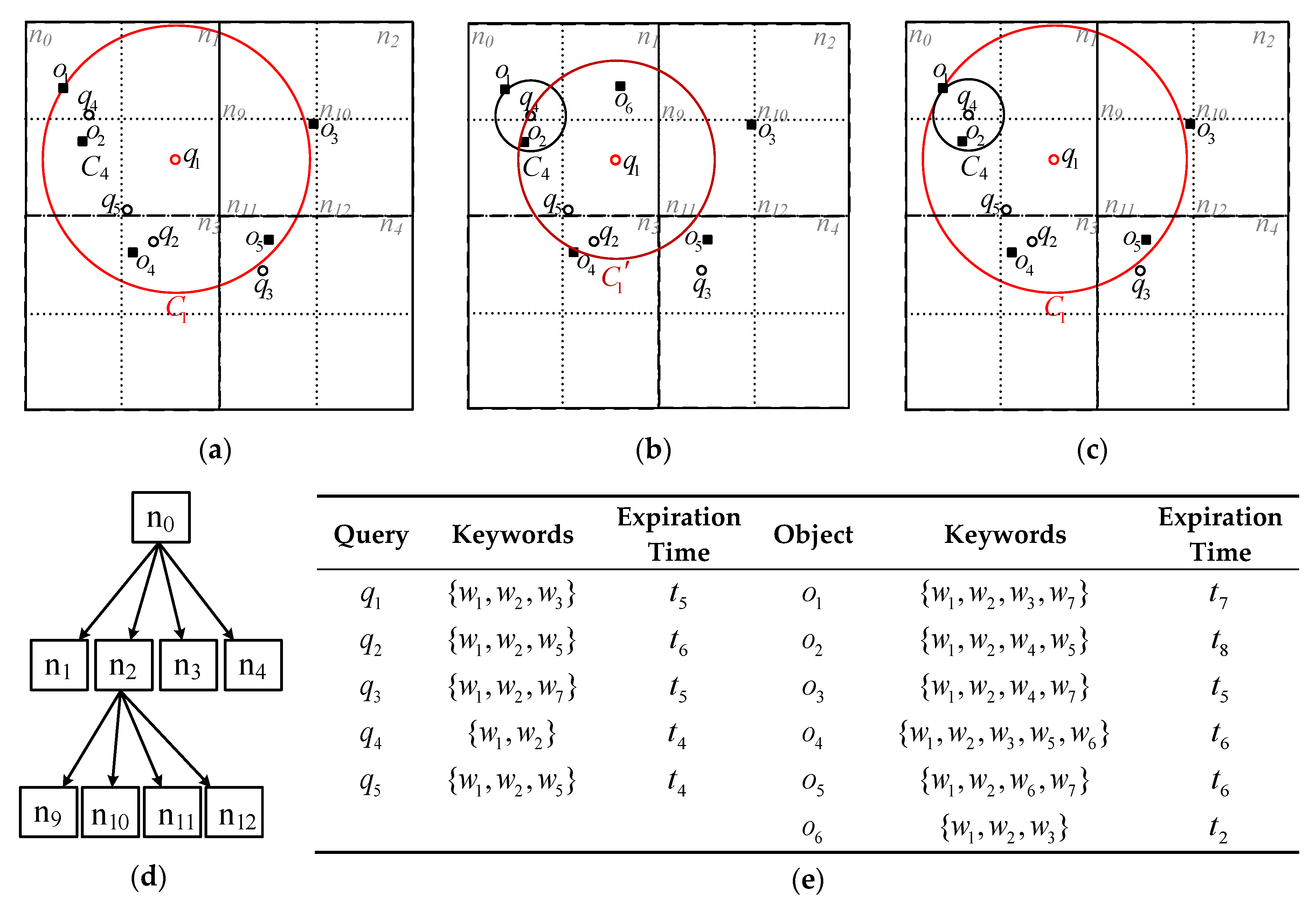
Example 1. Figure 1 depicts a running example used throughout this paper. At timestamp , there are five subscribed 2-NN (i.e., ) queries with a small circle representing their geo-location, and five objects with a small square representing their geo-location in Figure 1a, while corresponding keywords and expiration times are shown in Figure 1e. The spatial region is organized by a three-layer quadtree, where the spatial nodes are numbered successively, and the root node is . Taking the evaluation of as an example, is returned. For , the spatial search range, thereafter “search range”, is defined as a minimal circle centered at the geo-location of and covering , i.e., . At timestamp , an object arrives, as shown in Figure 1b, with keywords and expiration time . contains all the keywords of and , but only is hit by . The result and search range of are updated to and the circle , respectively, while the result and search range of are not affected. At timestamp , expires. For , the number of qualified objects in is less than 2, so the result should be re-evaluated. The result and search range of are updated to and the circle , respectively. Therefore, for CkQST, the spatial search range covering kNN objects changes dynamically with the arrival and expiration of qualified objects.
Challenges. The solution framework for evaluating generic continuous queries over spatial–textual data streams consists of selecting an appropriate spatial index and a textual index to form a hybrid spatial–textual index, and exploiting it with appropriate spatial and/or textual filtering strategies to process the incoming objects according to the features of queries [1,2,3,4,5,6,7,8,9,10,11,12]. There are three key challenges in constructing such an index for CkQST.
First, regarding the spatial filtering, evaluating CkQST is essentially identifying queries whose search range is hit by the incoming objects. It is very important to efficiently organize the search ranges of CkQST; therefore, how to map the search range of CkQST to the spatial nodes is the focus. The search range of CkQST covering kNN objects changes frequently with the arrival and expiration of qualified objects, which requires the index to have both strong filtering ability and low update cost. For most spatial indexes, having strong filtering ability and low update cost are contradictory. There are two approaches to mapping the search range of queries to spatial nodes to improve the filtering ability and reduce the update cost of the index. (1) Queries are mapped to the leaf nodes in the spatial index, which minimizes the spatial region of the nodes covering the search range of queries to reduce the number of objects to be verified [2,5,7,8,9,10,13,14,15]. (2) Queries are mapped to the spatial nodes according to the spatial distribution [10,11,12], the keyword distribution [6], or the corresponding cost model [1,3,4]. These approaches are appropriate in the scenarios where the search range of the queries rarely changes, but inappropriate to CkQST, where frequent update of the search range of the queries results in high costs.
Second, regarding the textual filtering, evaluating CkQST is essentially identifying queries whose keywords are fully contained in a given object. An inverted index is usually used to organize continuous queries [1,2,6,10]. A large number of queries make the posting lists very long, and the fast-arriving objects are verified against the corresponding posting lists in multiple rounds in a short time, which becomes the bottleneck of textual filtering. There are three ways to improve textual filtering capabilities. (1) Insert queries into the shortest posting list according to the frequency of query keywords to reduce the number of queries in posting lists, such as in the ranked-key inverted index [1,6]. The posting lists may still be long. (2) Increase the depth of textual partition, such as the ordered keyword trie [3,4,6]. It takes much time to construct the index, and nodes must be reconstructed if queries are updated, which is not appropriate for the scenarios like CkQST where the queries are frequently updated. (3) Organize queries in posting lists in the ascending order according to the ranking score [10]. However, there is no corresponding concept in CkQST. None of the above approaches can efficiently support CkQST textual filtering.
Third, the kNN re-evaluation is frequently triggered by object expiration. When an object expires, several CkQST have to be re-evaluated from scratch, which is expensive. Several techniques have been proposed to solve the similar problems in approximate top-k query (e.g., [10,13,16,17]). They all favor maintaining more than results to reduce the chances for re-evaluation. However, they either maintain all the skyline objects in the entire region [13,16], or maintain a k-skyband containing skyline objects whose scores were larger than a threshold [10,17], which are not designed for the CkQST returning exact results.
In view of the challenges, we extend a quadtree with an ordered, inverted index to organize CkQST. Three key techniques are proposed to exploit the spatial–textual index and address the above three challenges. The contributions of this paper follow.
(1) To support the frequent change of search ranges of CkQST, a memory-based cost model is proposed to map the search ranges of CkQST to the quadtree nodes, which minimizes the verification cost and index update cost.
(2) To reduce the number of queries verified and process objects in batches, an adaptive block-based ordered, inverted index is proposed to organize the query keywords at quadtree nodes, which allow multiple objects containing common texts to be verified concurrently. For this index, an insertion strategy is proposed to adaptively insert queries in views of the skewed distributions of CkQST and objects.
(3) To reduce the re-evaluation cost, a cost-based k-skyband technique is proposed to judiciously determine the search range for CkQST according to the workload of objects, which minimize the verification cost, update cost, and the re-evaluation cost.
The experiments on real-world and synthetic datasets demonstrate that the proposed techniques can efficiently evaluate CkQST. Compared with the state-of-the-art techniques, when the number of CkQST reaches 20 M, the average index updating time caused by incoming objects decreases by 61%, and the average incoming object processing time decreases by 36%. Compared with the re-evaluation from scratch, the average processing time for expired objects decreases by 99.99%. The rest of this paper is organized as follows. Section 2 formally defines CkQST and presents a framework for evaluating CkQST. Section 3 presents three key techniques for evaluating CkQST. Section 4 reports the experimental studies. Finally, Section 5 concludes this paper.
2. The Framework for Evaluating CkQST
In this section, we formally define CkQST in Section 2.1 and present a framework to evaluate CkQST in Section 2.2.
2.1. Problem Definition
A spatial–textual object is defined as , where is the geo-location, is a set of keywords (terms) from a vocabulary set , and is a timestamp indicating the expiration time of . All the spatial–textual objects over the data streams are denoted as . A CkQST is defined as , where , , and follow the similar meaning to , is the number of returned objects, i.e., at most (abbreviated as ) results are maintained for . The result list of , denoted as , contains a set of objects, each of which covers all the keywords in . is organized by a linked list, in which objects are arranged in the ascending order according to the distances to . Formally, , where is the Euclidean distance between and . Let be the distance between and its nearest neighbor result. The search range for , denoted as , is defined as a circle centered at with radius .
Spatial–textual objects are usually advertisements published by merchants or the latest breaking news, and CkQST are users’ search requests. Hereafter spatial–textual object and CkQST are abbreviated as object and query, respectively, if there is no ambiguity. To simplify the calculation, the terms in the vocabulary set are mapped to integers between 1 and according to the alphabetical order, where is the number of terms in . We assume that the terms in , and the terms contained in queries and objects are sorted in increasing order. Specifically, for , we use to denote the keyword of , to denote a subset of , i.e., , to denote , to denote , and to denote the number of keywords in . Objects follow the similar notations. Table 1 summarizes the notations used throughout this paper.
Problem Statement. Given a set of CkQST and spatial–textual data streams , for each CkQST, find the kNN objects containing all the query keywords over whenever objects arrive or expire.
2.2. The Framework for Evaluating CkQST
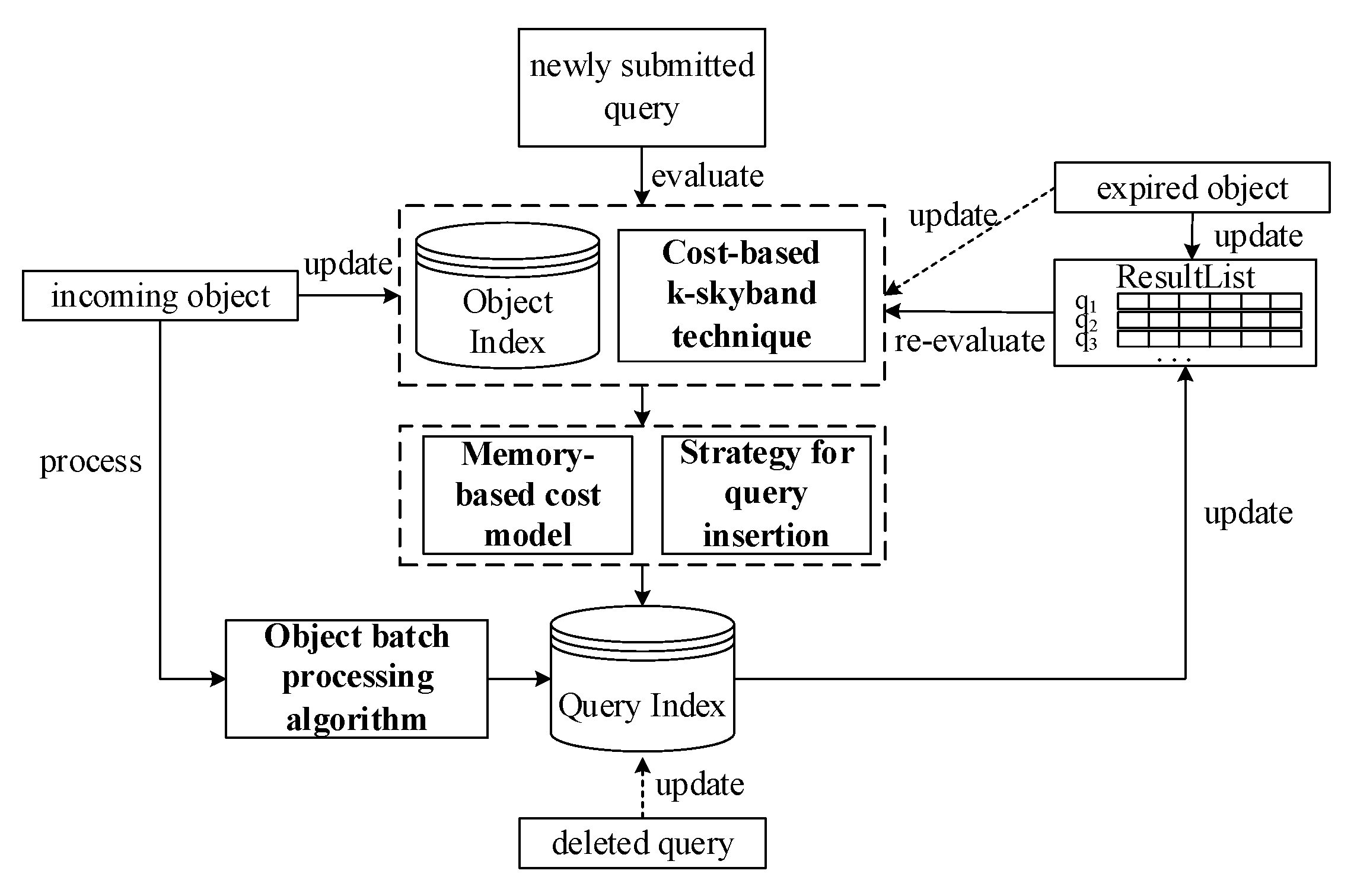
The framework for evaluating CkQST shown in Figure 2 consists of two indexes and four key techniques. The object index organizes the objects and can be implemented with any existing spatial–textual index, and we adopt the inverted linear quadtree (IL-quadtree) [18] as an example. The query index organizes queries, which is essentially a quadtree integrated with an ordered, inverted index described in Section 3.
The arrival and expiration of objects. When multiple objects arrive in a batch, they are inserted into the object index, and processed by the object-batch processing algorithm with the help of the query index to find all the affected queries and update the corresponding queries’ results and search ranges. When objects expire, the result list of affected queries is checked. Those queries that cannot be refilled through their result list are re-evaluated from scratch against the object index. To save computational cost, the expired objects are removed lazily from the object index until they are accessed again.
The arrival and deletion of queries. When a new query is submitted, it is initially evaluated using the object index with several strategies. A cost-based k-skyband technique is used to find an optimal search range for the query to reduce the cost for updating the index by sacrificing a little bit of filtering performance. A memory-based cost model is used to get the corresponding mapped spatial nodes. An adaptive insertion strategy is used to get the posting list and the corresponding block to be inserted. These strategies can further improve the filtering performance of the index and reduce the cost for updating the index. When a query is deleted or its search range shrinks, a flag is set in the corresponding nodes, where a query table is maintained, and it is not removed from the query index until accessed again, which is called delayed deletion and is necessary in an update-friendly system. A query insertion request might cancel the marked items, which avoid the deletion of objects changing frequently. If a query is deleted, its result list is also removed.
3. The Query Index
According to the above discussions, the query index is essentially a quadtree extended with an ordered, inverted index. Three techniques are proposed to enhance the filtering ability and reduce the update cost of the index. Section 3.1 introduces the motivations. Section 3.2 describes the ordered, inverted index, followed by a detailed adaptive query inserting algorithm in Section 3.3. Section 3.4 proposes the memory-based cost model to quantitatively analyze how to find optimal associated nodes for CkQST. The algorithm for processing objects in batches is presented to improve the throughput in Section 3.5. The re-evaluation technique is introduced in Section 3.6.
3.1. Motivations
Organizing the search range of CkQST. The first issue of using a quadtree to organize the search range of CkQST is how to map the search range to the quadtree nodes. Given that , can be mapped to any set of quadtree nodes , only if the union of the spatial region corresponding to these nodes in covers , which is also called that is associated with . Associating a query with the quadtree nodes is challenging because it affects two computation costs: (1) Verification cost, i.e., the cost of verifying the query with the objects falling in the associated nodes. (2) Update cost, i.e., the cost of inserting or deleting the query in or from the associated nodes. If the search range is organized by nodes with large regions, the index update cost is small, and the verification cost is large; otherwise, if multiple nodes with small regions are used, the situation is reversed. Therefore, a cost model is required to trade off the verification cost and update cost, and find the optimal associated nodes for CkQST.
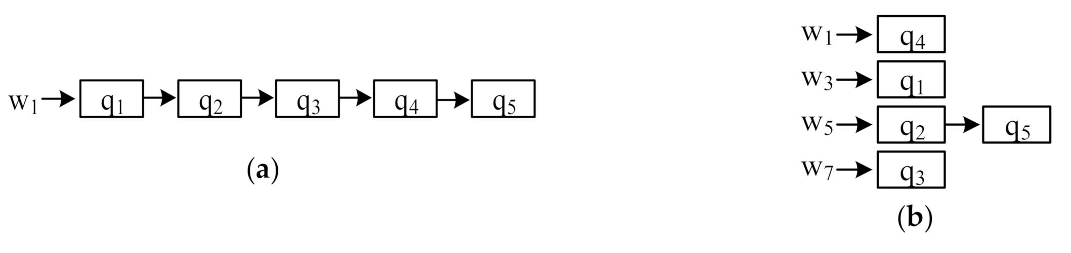
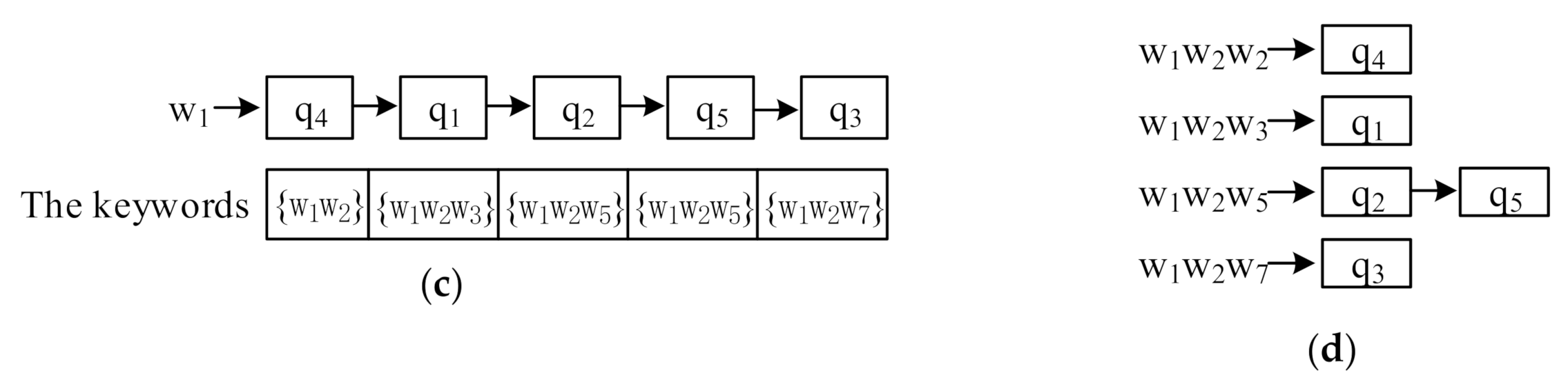
Organizing the keywords of CkQST. When new objects arrive, the cost of verifying these objects with queries in spatial nodes is expensive. How to reduce the verification cost is the key to improve the filtering ability of the index. We discuss three aspects of constructing an inverted index. (1) For an inverted index, queries in posting lists are usually unordered. For the five queries in Figure 1, we attached them to the posting list of a single keyword. Figure 3a is the inverted index in which queries are attached to the posting list corresponding to the first query keyword, and Figure 3b is the ranked-key inverted index in which queries are attached to the posting list corresponding to the least frequent keyword. If the incoming objects contain the corresponding term, all queries in posting lists are verified [1,2], which is inefficient. In this work, we use an ordered, inverted index to solve the above problem. Figure 3c is the ordered, inverted index if queries are attached to the posting list corresponding to the first keyword, i.e., queries in posting lists are organized in the ascending order according to the keywords. When with keywords arrives, the posting list corresponding to is verified. When is verified with , its keywords are smaller than , so we can terminate the verification early and speed up processing objects.
(2) Compared with the ordered, inverted index constructed by single keyword, the ordered, inverted index constructed by multiple keywords has more advantages. The length is shorter and the verification probability is smaller. As Figure 3d shows, is verified with the first two posting lists and contains all the keywords of the queries in these posting lists. However, the number of posting lists might grow sharply. If the number of terms contained in vocabulary set is 1 M, and the number of query keywords are not more than 5, total 106×5 posting lists are required, which is difficult to implement by hash table due to the need for large continuous memory. Like other works in [1,2,3,4,5,6,7,8,9,10,11,12], this paper uses the Map class in Microsoft Visual Studio [19] to build the ordered, inverted index. Lemma 1 describes the verification efficiency with the number of keywords for constructing the ordered, inverted index. Section 4.2 verifies this lemma through experiments. Based on the discussions, we select two keywords to construct the ordered, inverted index.
(3) Usually, there are many queries in posting lists, but only a small number match the incoming objects. Therefore, quickly locating the queries to be verified in posting lists is another way to improve the efficiency of evaluating CkQST. The queries in posting list are partitioned into multiple blocks such that objects are verified with the queries in a few blocks rather than the whole posting list. The only problem is how to partition these queries in posting lists. It is inefficient to have too many or too few queries in a block. An adaptive insertion strategy is proposed in Section 3.3.
3.2. Ordered, Inverted Index
The formal definition of an ordered, inverted index constructed using two keywords follows. Queries are attached to the posting list of their first two keywords, and arranged in ascending order according to their keywords.
Definition 1 (Ordered Posting List/Ordered, Inverted Index).
Given a set of queries to be inserted into a quadtree node, if , and , the posting list determined by the two terms at the node is denoted as , in which these queries are successively inserted. is called an ordered posting list. Specifically, if these queries only contain one keyword, the corresponding posting list is denoted as. All the ordered posting lists constitute the ordered, inverted index.
Hereafter the ordered posting list is abbreviated as posting list, if there is no ambiguity. To quickly locate the queries to be verified, posting lists are divided into multiple blocks.
Definition 2 (Block).
Given any ordered posting list ,, is the block of . For any query in,, where , . denotes all the keywords satisfying . Specially, if only contains one or two keywords, it is inserted into the block of the corresponding posting list.
Lemma 1.
If the number of keywords for constructing an ordered, inverted index is
, there are at mostposting lists at a node. For any object containing more than two keywords, the verification cost can be estimated by Equation (1). Where is the number of blocks in a posting list, is the number of queries in , contains queries whose keywords are contained in , and the number of keywords is less than . The proof is shown in Appendix A.
For , the verification probability, denoted as , is maintained, i.e., the probability of verifying these queries subjected to in . For , the verifying probability, denoted as , is maintained, i.e., the probability that the block is verified, which can be estimated by Equation (2).
The following theorems claim that the incoming object is verified with few queries in posting lists. For any incoming object, the blocks being verified can be located according to block keyword interval (see Theorem 1). The object verification with a block or a posting list can be terminated if the keywords are smaller than that of some query being verified. (see Theorem 2).
Theorem 1.
Givenand a posting listbeing verified with, forin, ifin, contains all keywords of, only if, .
Proof.
Suppose that contains all the keywords of , but there is no term in satisfying . Based on Definition 2, , does not contain the third keyword of , so does not contain all the keywords of . It is contradicted by the hypothesis, so the theorem is proved. □
Theorem 2.
Givenand a posting listbeing verified with, forin, we have the following conclusions. (1) If, is not the result of queries in the blocks starting from, andcan be terminated verifying. Specifically, for in , if , can be terminated verifying. (2) If , is not the result of queries in .
Proof.
(1) If , i.e., for any in , does not contain its third keyword, is not the result of . So does the block , since . Similarly, for any in , , is not the result of queries after .
(2) If , is not the result of the queries in . □
3.3. Adaptive Query Insertion Algorithm
Given any posting list at a node, we consider two extreme situations: (1) the posting list only contains a block which contains all queries; (2) the posting list contains many blocks, each of which only contain one query. The former has poor filtering ability and the latter has high update cost. Neither is what we expect. In the real world, people are concerned with different interests and often pay high attention to the breaking news or topical issues, so the keywords of the queries and objects vary over time. For each query, we adaptively insert it into the posting lists according to the historical queries and objects. We expect that the increase of the verification cost and update cost of the posting list is minimal after the query being inserted.
Given a posting list , the update cost is denoted as , and the verification cost is denoted as , which can be estimated by Equation (3), where represents the verification cost of the block in .
Theorem 3.
Letbe the query to be inserted into, , hasblocks, is the increase of verification cost ofafterbeing inserted. We have the following conclusions.
Case 1: If satisfies , is inserted into . .
Case 2: If satisfies , but satisfies , is inserted into the tail of . The updated block is denoted as . .
Case 3: Similar to case 2, if satisfies , but satisfies , is inserted into the head of the . .
Case 4: If satisfies , a new block is constructed in , and is inserted into ..
Proof.
(1) Case 1: If is inserted into , the verifying probability does not change since , but the number of queries in increases by 1.
(2) Case 2:
(3) Similar to case 2.
(4) Case 4: For any in , ,
Theorem 3 shows all the cases where the verification costs increase if a query is inserted into the posting list. The increase of update costs corresponding to the above four cases are , , , and respectively. To compare the verification costs and update costs, we introduce a normalization parameter to represent the ratio of the update operation to the verification operation, i.e., if a query is inserted into a node, there will be objects being verified with it. A query is adaptively inserted into the posting list according to the following theorem. □
Theorem 4.
Let be the query to be inserted into, . Ifin satisfies , is inserted into. Otherwise, the minimumof the cases 2–4 is taken.
| Algorithm 1: |
| 1 if then |
| 2 construct new block b in insert q into b; return; |
| 3 ; |
| 4 if then q is inserted into br; return; |
| 5 if and then |
| 6 q is inserted into br−1; return; |
| 7 if then compute on ; |
| 8 if r == 1 then compute ; |
| 9 if r > 1 then compute ; |
| 10 if case 2 then q is inserted into the tail of br−1; |
| 11 if case 3 then q is inserted into the head of br; |
| 12 if case 4 inserted into a new block. |
Given , if contains no more than two keywords, it is directly inserted into the of the corresponding posting list. Algorithm 1 shows how a query containing more than two keywords is adaptively inserted into a posting list. If does not exist, a new block is constructed, and is inserted into (lines 1–2). Otherwise, a block in is found for to minimize (lines 3–12). First, we find the block, denoted as , whose is the smallest—no smaller than (line 3). If , is inserted into (line 4). If (), is inserted into block (lines 5–6). Otherwise, we compute according to cases 2–4 in Theorem 3 and select the minimum case (lines 7–12). It is worth noting that when compared with the first block of the list, there are only cases 3–4, and if is larger than of all the blocks, there are only cases 2 and 4.
Computation complexity. In the worst case, the computation cost of Algorithm 1 is shown as Lemma 1. That is, in posting lists constructed by two keywords, the complexity of inserting a query at a node is . The algorithm can adaptively adjust and .
3.4. The Memory-Based Cost Model
A memory-based cost model associates queries with the optimal quadtree nodes. Given the search range of CkQST, the model traversals the quadtree from the root node, compares the sum of the verification cost and index update cost if the query is associated with the current node and its child nodes, and selects the smaller one. The verification cost is the product of the number of verified objects and the expectation of the verification cost, and the update cost is the expectation of the update cost if the query is inserted into the corresponding block of the posting list.
Definition 3 (Minimum Bounding Node).
Given
and search range , if ,, and for any child node of ,, is the minimum bounding node of , where , are the region where and locate respectively. The minimum bounding node of is the node, which covers its search range, but any of its child nodes cannot completely cover the search range.
Verification cost. Given and its minimum bounding node , , if is associated with , the verification cost within unit time interval, denoted as , can be estimated by Equation (4). We assume that the query and object contain more than two keywords, and the average verification cost is unit time.
Specifically, if the query or the object contains one or two keywords, the verification cost is estimated by Equation (5). This case is simple, so we omit the details.
where is the number of objects falling in within the unit time interval. is the probability that is verified if it is inserted into in , i.e., the probability that the objects contain the terms , and , and can be estimated by Equation (6).
where is the number of keywords contained in . is the verification cost if is inserted into in , and can be estimated with the expectation of verification cost of the queries in , i.e., Equation (7).
where is the number of queries subjected to in . Similarly, if the query is associated with a set of non-overlapping nodes, denoted as , the verification cost is denoted as and can be estimated by Equation (8).
For , we find the optimal associated nodes starting from its minimum bounding node, and check whether the query is associated with the current node or associated with its child nodes. The difference of two verification costs is estimated by Equation (9).
where keeps the intermediate result, contains the child nodes of that intersect with the search range of the query. It is worth noting that if , we terminate the iteration.
Update cost. When inserting or deleting queries in nodes, it will incur an index update cost. We delay deleting queries until these queries are accessed again, so the deletion cost is ignored. If a query is associated with its minimum bounding node , and is inserted into a block of posting list in , the insertion cost consists of two parts, the time to find the corresponding block and the time to find the insertion position. The update cost, denoted as , can be estimated by Equation (10).
If is associated with a set of non-overlapping nodes, denoted as , the update cost is denoted as and can be estimated by Equation (11).
Similarly to , the difference of two update costs between the query being associated with the node and associated with the child nodes is estimated by Equation (12).
Given and search range , we start from the minimum bounding node, and computes and between the query being associated with the node and associated with the child nodes. If , the child nodes are the optimal. Otherwise the node is optimal. The computation cost consists of two parts, finding the minimum bounding node of , and finding an optimal association in the descendant nodes of minimum bounding node. The computation cost of the first part is , and the second part is , i.e., in the worst case, the node will be partitioned until the leaf node, where is the height of the quadtree.
3.5. Processing Objects in Batches
For these objects being verified with the same posting list, an object processing algorithm, which is a group matching technique that follows the filtering and verification strategy, is proposed to process objects in batches.
A data structure is defined to group the objects being verified with the same posting list, where is the block id, is a term, is a set of objects being verified with block and containing . For the convenience of the description, is a set of terms satisfying , is a set of objects which are verified with the queries in block and contain .
Algorithm 2 describes how to process a set of objects represented by , which are verified with the queries in the posting list . If is , the queries in is verified with the objects in (lines 1–5). Otherwise, for any term in , according to Theorem 2, if , we check the next term (line 7); if , we check the next block (line 8); otherwise, for each query in , if , we check the next term (line 10); if , we check the next query (line 11); otherwise, we verify whether the object is the results of . If yes, is added to (lines 12–13). Moreover, the result list and search range of are updated.
Computation complexity. Algorithm 2 describes how to process objects in batches in an ordered posting list. In the worst case, objects are processed individually. As Lemma 1 shows, in posting lists constructed by two keywords, for an object, the time complexity of finding the qualified queries at a node is .
| Algorithm 2: . |
 |
3.6. Cost-Based k-Skyband Technique
To reduce the re-evaluation cost, a cost-based k-skyband technique is proposed to judiciously determine an optimal search range for CkQST such that the overall cost defined in the cost model can be minimized. Specifically, for , three parameters are defined: an extended search range is denoted as , where ; a k-skyband, i.e., an extended result list, denoted as , where ; the number of objects containing all query keywords within in the initial timestamp is denoted as , where .
Definition 4 (Loose Matching).
Given and , loosely matches only if and . All the objects that loosely match aredenoted as .
Definition 5 (Dominance).
Given and two objects ,, which loosely match , dominates only if and or and .
Definition 6 (k-skyband/Extended Result list).
Given , for any incoming object , we insert it into the k-skyband only if: (1) loosely matches ; (2) is dominated by less than other objects. For, ifan object loosely matches , and there are objects in dominating,would not be a result at any timestamp. Therefore, we would not insert these objects into the result list.
Theorem 5.
Given and an extended search range, we always have the following conclusions. (1); (2); (3)iff.
Proof.
(1) At any timestamp, for , we have and , i.e., loosely matches , and less than objects dominate . So . (2) According to Definition 4, for , loosely matches , so , . (3) Since , if , we have . On the other hand, if , , i.e., and , which means loosely matches , but is dominated by more than other objects, which is contradicted by . The theorem is proved. □
According to Theorem 5, the extended result list is the super set of the exact result list, from which we can extract the kNN objects, and the number of objects in extended result list is less than only if the number of objects in is less than .
Given , an extended search range , and the corresponding extended result list , three costs are defined in the cost-based k-skyband technique: the verification cost of within , the update cost of , and the re-evaluation cost.
Verification cost. The verification cost of within , within the unit time interval, denoted as , is estimated by Equation (13), i.e., the verification cost if is inserted into all the leaf nodes that intersect with .
Update cost. Similarly to , the extended result list is organized by a linked list. For , a dominance counter is defined to count the number of objects dominating . If an incoming object is inserted into , the dominance counters of all the objects in with and , or and will increase by 1, and the objects with dominance counter equal to will be evicted, which can be processed in time. When an object in expires, it is deleted from until it is accessed again. The cost is negligible. The update cost of within unit time interval, denoted as , is estimated by Equation (14). Where is the number of object updates within unit time interval, is the probability that the objects loosely match within the search range , and is estimated by , is the probability that a qualified object arrival, can be estimated by .
Re-evaluation cost. The re-evaluation cost within the unit time interval is denoted as . Where is the re-evaluation period, i.e., the shortest time required between two consecutive independent evaluations, and is the frequency of re-evaluation. is the re-evaluation cost, and is approximated to the verification cost in , i.e., .
The overall cost in the cost-based k-skyband technique, denoted as , is shown in Equation (15). When is minimal, the search range is optimal.
In the following, we discuss how to get . is the re-evaluation period, i.e., the shortest time that is reduced to since the last re-evaluation. For , the update process of number of objects in can be modeled as a simple random walk, which is a stochastic sequence , with being the original status, defined by , where is the object update, which is an independent and identically distributed random variable. In , if an object is inserted, ; if an object expires or is dominated, ; otherwise . It’s difficult to estimate due to the eviction of objects by the dominance relationship in . For example, an object is inserted, but the number of objects decreases due to the eviction of objects with dominance counters reaching . According to Theorem 5, the number of objects in is less than only if the number of objects in is less than , and the objects in don’t dominate each other. Therefore we estimate the shortest time that is reduced to , denoted as , where . The object update in at any timestamp can be estimated as Equation (16).
The number of object updates required to reduce the number of objects from to in , denoted as , is estimated by Equation (17). is estimated by .
For , the variables in Equation (15) are and . To minimize Equation (15), we employ the incremental estimation algorithm to compute the optimal and the corresponding .
To accommodate our extended search range with the objects processing algorithm and index construction and maintenance algorithm, we replace with and replace with .
4. Experiments
In this section, we conduct a set of comprehensive experiments to evaluate the efficiency and scalability of the key techniques. Section 4.1 introduces the experimental environment. Section 4.2 evaluates the effect of three tuning parameters and the re-evaluation technique. Section 4.3 evaluates the efficiency and scalability of our index techniques.
4.1. Experimental Settings
All experiments are implemented in VC++, and run on a Win10 machine with an Intel I7-8700K 3.7 GHz CPU and 32 GB memory. In accordance with previous works (e.g., [2,3,4,5,6,7,8,9,10,11,12]), we load the query indexes into main memory to support real-time response.
Datasets. Three datasets are collected for experimental evaluations. The statistics are shown in Table 2. TWEETS contains twitters collected from Twitter [8]. TWEETS is the default dataset. GN is obtained from the US Board on Geographic Names, in which each record contains a geo-location and some terms (http://geonames.usgs.gov/). GOWALLA is a synthetic dataset, in which each record contains a geo-location collected from the Gowalla (https://snap.stanford.edu/data/loc-gowalla.html), and less than 50 terms randomly assigned from 20 Newsgroups (http://people.csail.mit.edu/jrennie/20Newsgroups). Based on the datasets, we generate queries and objects.
Query Workload. For each sample dataset, we take the geo-location as the geo-location of the query and randomly select terms of the sample data as the query keywords, where . The number of returned kNN results is set to a default value. At any timestamp, the expired queries are randomly selected.
Object Workload. For each sample dataset, we take all terms as the object keywords, and take the geo-locations deviating from the original geo-location by 0.01% to 1% of the maximum distance in the region. At any timestamp, the expired objects are randomly selected.
Set of Queries and Objects. For each dataset, unless otherwise specified, we select 5 M objects and queries to construct the query index and object index initially, and generate three test sets, each of which contains 2 M objects and 2 M queries. The evaluation criteria take the average performance of three test sets.
Baseline. We compare our index techniques with IQ-tree [1], Ap-tree [3] and FAST [6]. By default, for Ap-tree, the fanout, partition threshold, and KL-Divergence threshold are set to 200, 40, and 0.001. We use the number of verifications to replace the number of I/O in the cost model of IQ-tree. In the following sections, we use AOIQ-tree to represent the index integrated the quadtree with the ordered, inverted index, and three key techniques. We compare the cost-based k-skyband technique with the Kmax [16] when they are integrated in the AOIQ-tree.
Evaluation criteria. We report four criteria: (1) the index construction time (i.e., ICT), i.e., the time of inserting queries into index after finding their search range; (2) the average incoming object processing time (i.e., AOPT), i.e., the time of finding the affected queries and modifying their corresponding parameters when an object arrives; (3) the average index updating time caused by objects (i.e., AIUT), i.e., the time of updating query index after processing objects; (4) index size, i.e., the memory used for constructing the query index. By default, the number of keywords for constructing ordered, inverted index , the number of kNN results returned for CkQST , the height of the quadtree , the ratio of the update operation to the verification operation , and the number of object updates within unit time interval are set to 2, 20, 10, 0.001, and 20,000.
4.2. Experimental Tuning
In this section, a series of experiments are conducted to evaluate the effect of parameters in techniques on the AOIQ-tree.
Effect of . Figure 4 shows the evaluation criteria of the AOIQ-tree when takes 1, 2, 3, 4, and 5. According to Lemma 1, if is small, the number of queries in posting lists is large, so it takes a long time to verify queries in posting lists; contrarily, if is large, it takes a long time to find the posting lists to be verified. Therefore, the optimal is neither too small nor too large. As shown in Figure 4, when takes 2, the performance of the index is the best. The larger is, the larger the index size. When , the verification cost and update cost in a single posting list decrease, so the cost model maps queries to nodes with large regions, so ICT, AIUT and index size decrease, while AOPT increases.
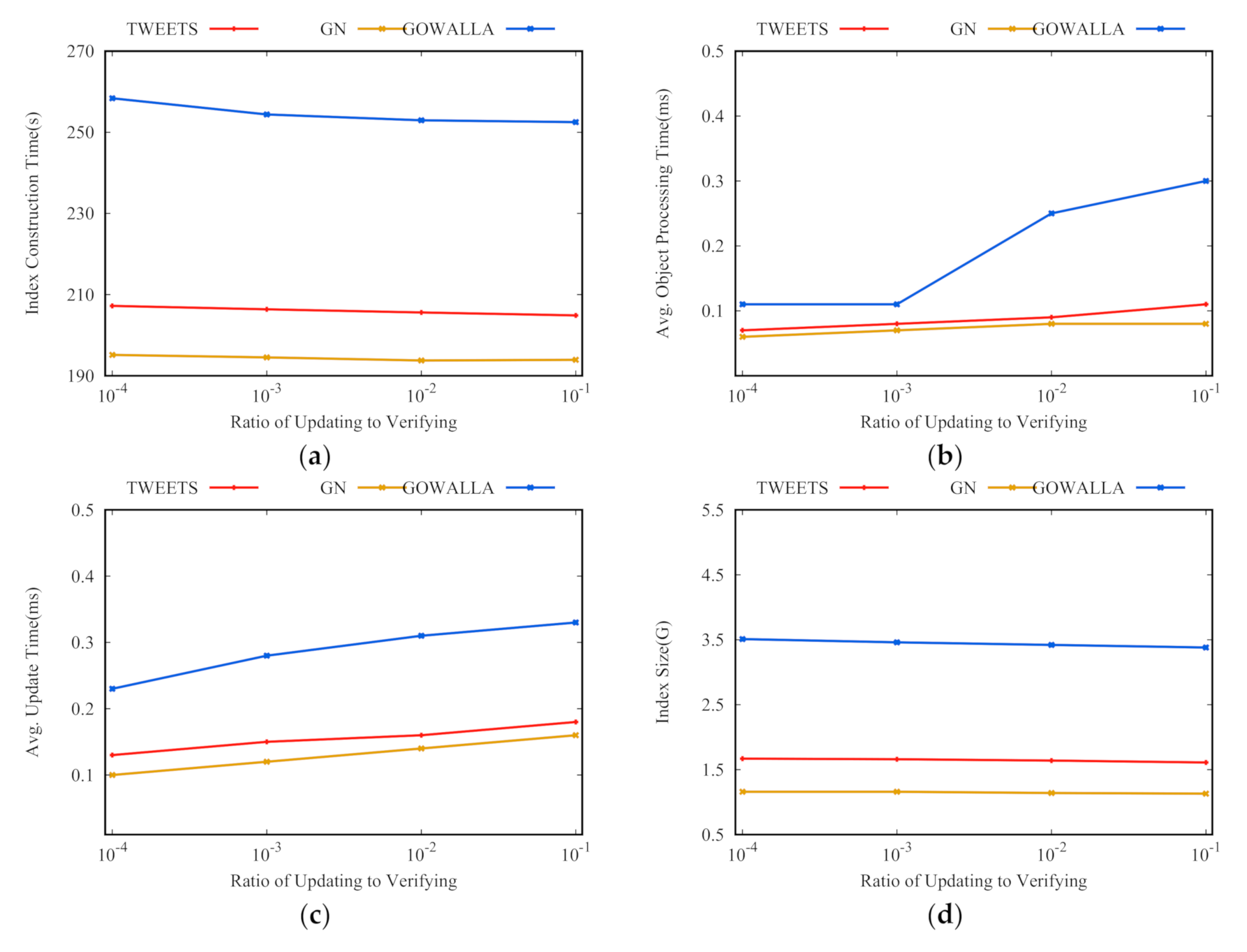
Effect of . Figure 5 shows the evaluation criteria of the AOIQ-tree when takes 0.0001, 0.001, 0.01, and 0.1. When takes 0.0001, the verification cost plays a major role in finding the associated nodes, therefore, queries are associated with many small nodes, so ICT is long, AOPT and AIUT are short, and index size is large. When increases, the index update cost is more important, so queries are associated with fewer larger nodes, so ICT and index size decrease, while AOPT and AIUT increase.
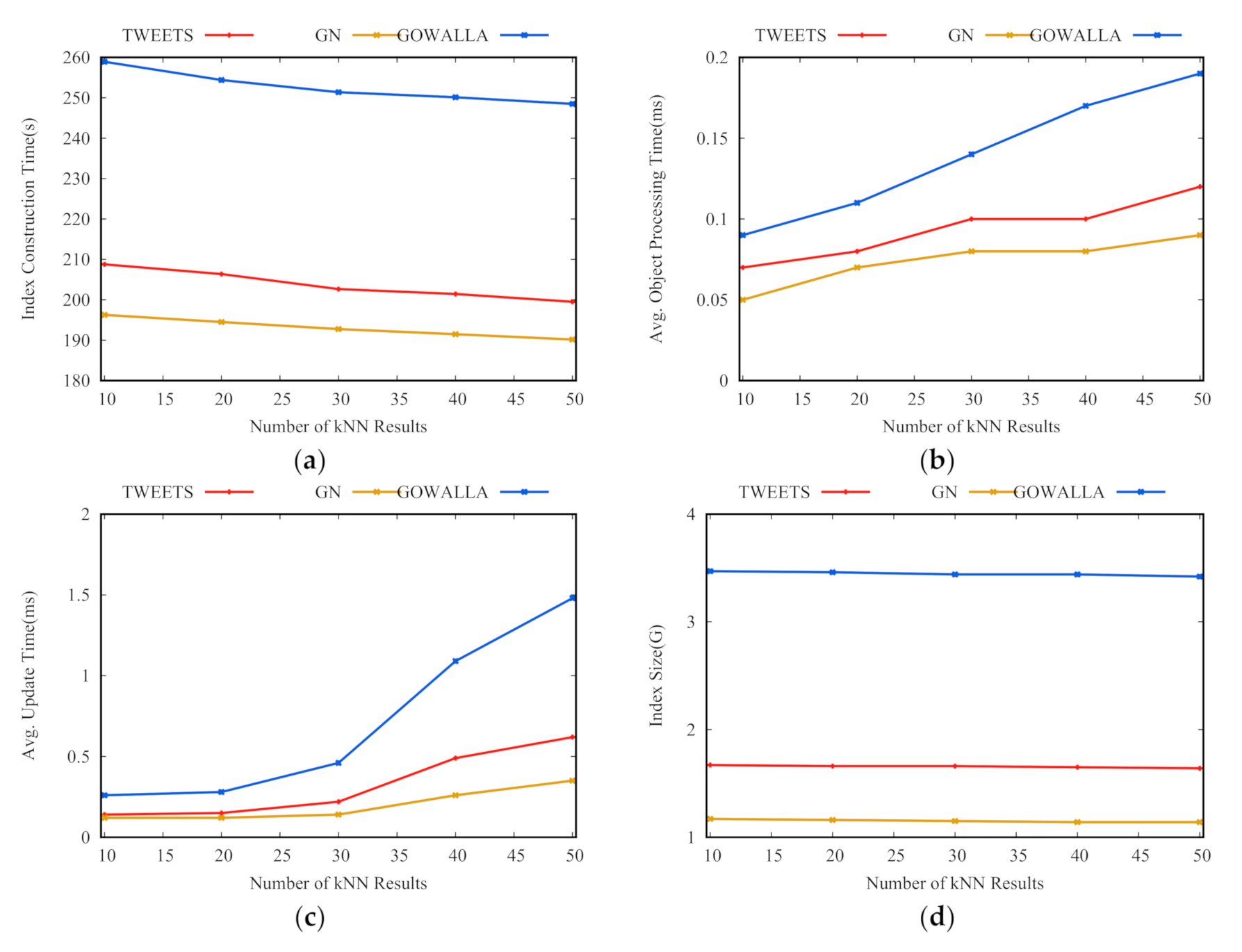
Effect of . Figure 6 shows the evaluation criteria of the AOIQ-tree when takes 10, 20, 30, 40, and 50. As is small, the number of returned objects for queries is few, the search range of queries is small, and queries are associated with many small nodes, so the ICT is long, AOPT and AIUT are short, and index size is large. On the contrary, when is large, the search range of the queries becomes larger, and queries are associated with few larger nodes, the ICT and index size decrease, and the AOPT and AIUT increase.
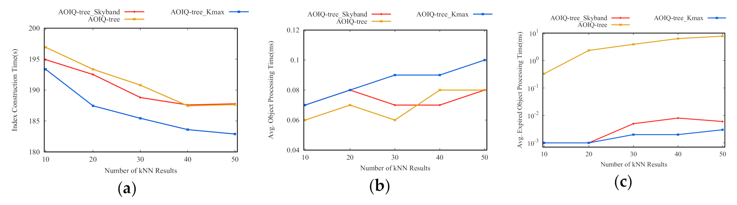
Effect of re-evaluation techniques. We evaluate the re-evaluation performance in three cases, denoted as AOIQ-tree, AOIQ-tree_Kmax, and AOIQ-tree_Skyband. AOIQ-tree only keeps objects in the result list, AOIQ-tree_Kmax keeps objects in the result list, and the number of objects in the result list for AOIQ-tree_Skyband is calculated according to the cost-based k-skyband technique. Figure 7 shows the ICT, AOPT, and EOPT in three cases with varied , where EOPT is the average processing time for expired objects, i.e., the average time of modifying the parameters of the affected queries or re-evaluating the queries if the number of objects in their result list is less than when an object expires. The number of objects maintained in AOIQ-tree_Kmax is more than AOIQ-tree_Skyband, which is more than AOIQ-tree. The ICT of AOIQ-tree_Kmax is shortest, and that of AOIQ-tree is longest. The AOPT of AOIQ-tree and AOIQ-tree_Skyband are shorter than that of AOIQ-tree_Kmax. The EOPT of AOIQ-tree_Kmax and AOIQ-tree_Skyband are shorter than that of AOIQ-tree. This phenomenon is related to the numbers of objects maintained in their result list. Compared with AOIQ-tree, the EOPT of the other two techniques are much less, and if takes 10, 20, the average update time is close to 0.
4.3. Performance Evaluation
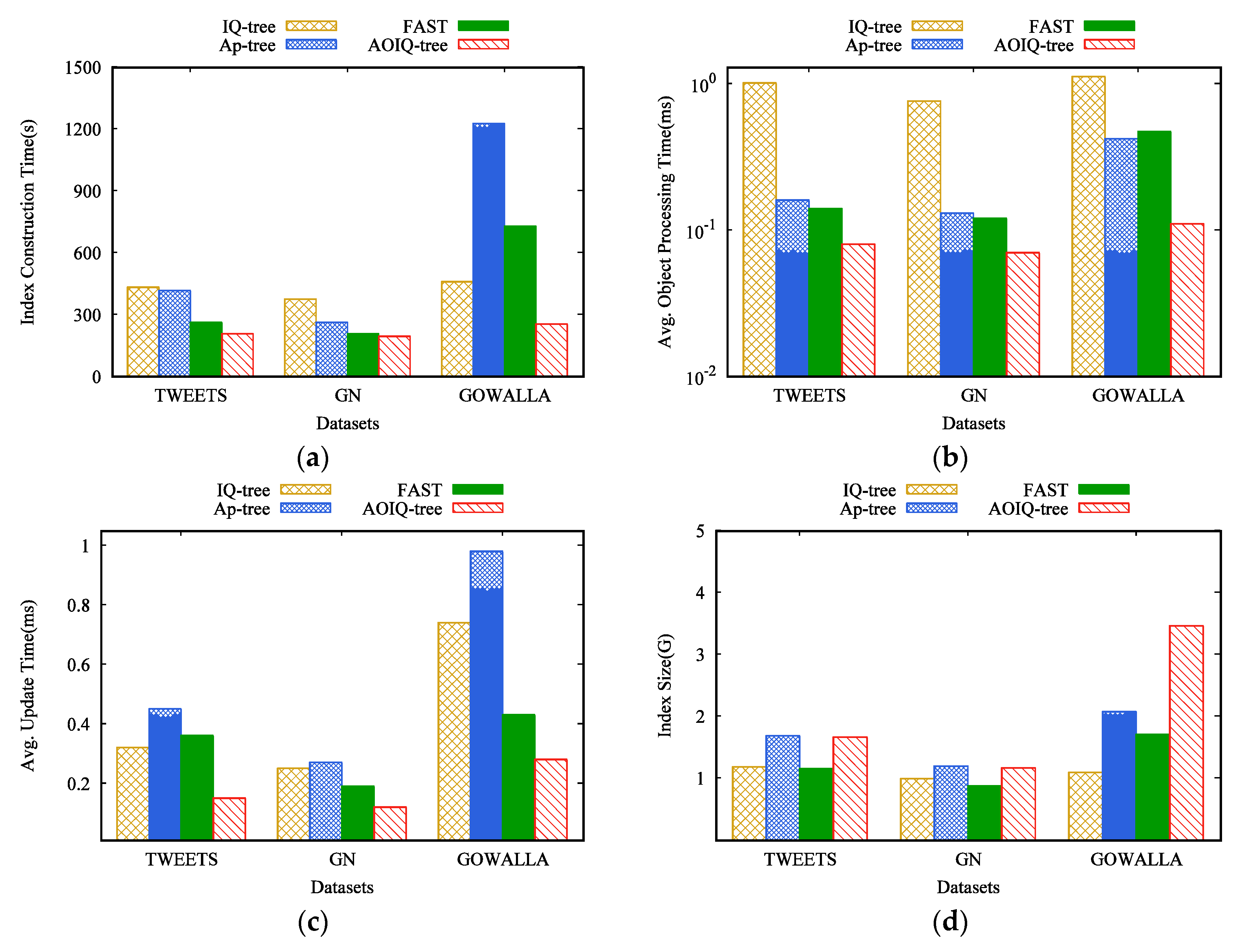
Evaluation on different datasets. We evaluate the efficiency of the key techniques against three datasets in Figure 8. The number of queries is 5 M. As shown in Figure 8, besides the index size, AOIQ-tree is always the best one. IQ-tree has a good spatial filtering performance, but its textual filtering ability is weak; AP-tree comprehensively considers the spatial and textual distribution of queries, but the index construction and update cost are expensive; FAST has a good textual filtering performance, but its spatial filtering ability is weak. The memory-based cost model in AOIQ-tree can minimize the verification cost and update cost, which makes the number of queries in spatial nodes neither too many nor too few; the ordered, inverted index in AOIQ-tree is constructed by two keywords, which makes the verification cost close to the ordered keyword trie, and the update cost close to the ranked-key inverted index. AOIQ-tree takes up the most memory, which is determined by the structure of its posting lists. The evaluation criteria of GN are the smallest, and Gowalla are the largest, which is because the data in Gowalla contain far more keywords than the other two datasets. For Gowalla, the AOPT of AP-tree is shorter than that of FAST. This is because a large number of queries in Gowalla only contain frequent keywords, compared with FAST, AP-tree comprehensively considers the spatial and textual distribution of queries, i.e., index filtering is more powerful, so AOPT is shorter.
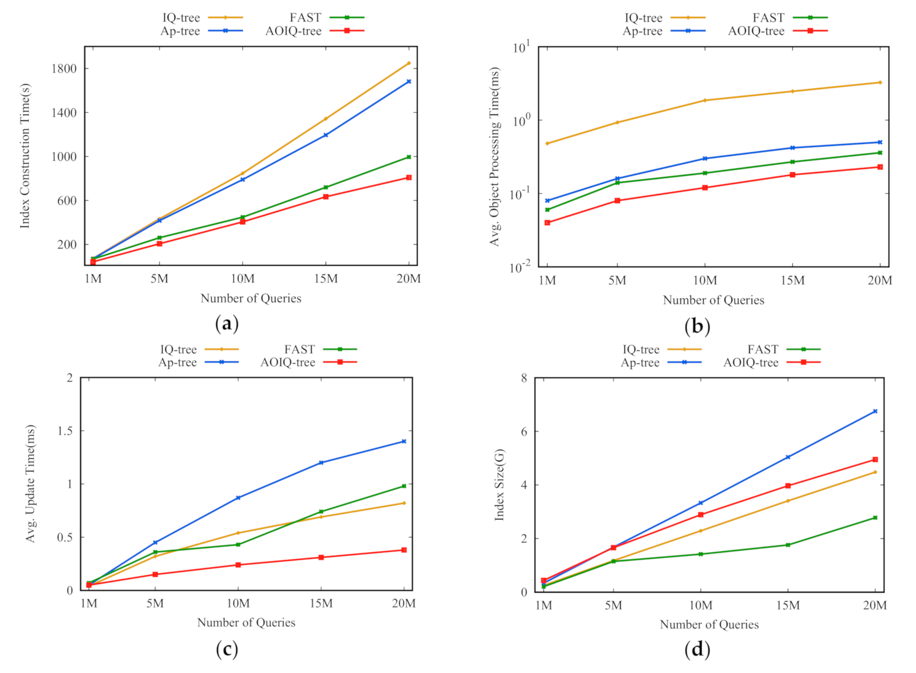
Effect of number of queries. To evaluate the scalability of the key techniques on the number of queries and objects, we increase the number of queries and objects from 1 M to 20 M to construct the object index and query index. As Figure 9 shows, the ICT, AOPT, and AIUT of all indexes increase as the number of queries increases, and AOIQ-tree is much more scalable. For instance, it only takes 0.23 ms on average to process the incoming objects when the number of queries reaches 20 M, which is 54% faster than Ap-tree and 36% faster than FAST. This shows that our techniques have good scalability. The AIUT of AOIQ-tree is the shortest, and Ap-tree is the longest. That’s because AOIQ-tree associates queries with optimal nodes to adapt to the objects on data streams, and some of the Ap-tree nodes are re-constructed if many queries updates in these nodes. Compared with AP-tree, only some queries update in FAST nodes, so AOIQ-tree’s AIUT is shorter.
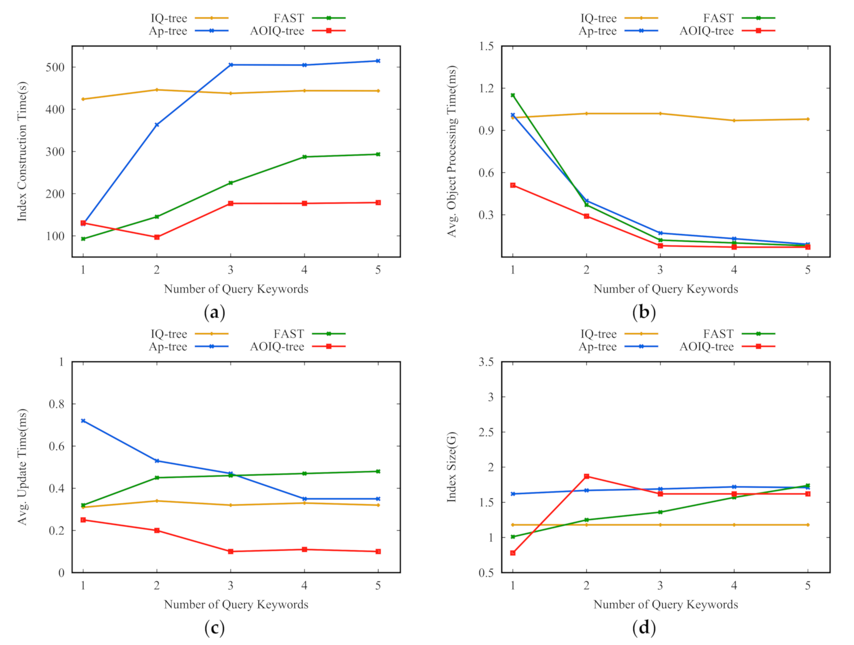
Effect of number of query keywords . To evaluate the scalability of key techniques on , we increase from 1 to 5. As shown in Figure 10, the evaluation criteria of IQ-tree are insensitive to the number of keywords since it focuses on the spatial distribution of the queries. Ap-tree, FAST, and our index consider the keyword distribution of the queries, so the evaluation criteria vary with . As increases, the ICT and index size increase, and the AOPT decreases. That is because Ap-tree continuously calculates how to partition queries into nodes according to query keywords, and increases the number of textual nodes and height of the tree. For FAST, as increases, more keywords being attached to posting lists become frequent, and queries are more likely to be inserted into the multiple higher-level nodes. For AOIQ-tree, the time of sorting the queries increases when the ordered, inverted index is constructed.
5. Conclusions and Future Research Perspectives
The challenging for evaluating CkQST is how to strike the balance between the filtering ability and the update cost of the spatial–textual index. To address the challenging, we use quadtree and inverted index to organize millions of CkQST with three techniques. A memory-based cost model maps the search range of CkQST to the quadtree nodes to balance the spatial filtering ability of the indexes and the cost for updating the indexes. The balance can be further tuned by the cost-based k-skyband technique, which judiciously determines the search range for CkQST according to the workload of objects. An adaptive block-based ordered, inverted index enhances the textual filtering ability. The experimental results on the real-world and synthetic datasets show that the proposed techniques are effective and scalable, and can significantly improve the evaluation efficiency of CkQST. The future work for evaluating the continuous query over spatial–textual data streams includes solving the challenges of continuous queries in mobile and other relevant scenarios, and exploring efficient evaluation techniques using hardware technologies such as Graphics Processing Unit and distributed clusters and trade-off strategy for precision and evaluation efficiency.
Author Contributions
Rong Yang proposed the methods, implemented the algorithms for the experiments, and wrote the manuscript; Baoning Niu provided suggestions for the methods and experiments, reviewed and modified the manuscript. All authors have read and agreed to the published version of the manuscript.
Funding
This research was funded by the National Natural Science Foundation of China (Grant No. 62072326), National Key Research and Development Plan of Shanxi Provence (Grant No. 201903D421007).
Acknowledgments
The authors would like to thank three anonymous reviewers for their valuable suggestions and comments.
Conflicts of Interest
The authors declare that they have no conflict of interest.
Appendix A
In the proof of Lemma 1, without loss of generality, we suppose that all the terms in are contained in different blocks and divide the object processing at quadtree nodes into three steps: finding the posting lists to be verified, finding the blocks to be verified in all posting lists, and finding the queries to be verified in all blocks.
Proof of Lemma 1.
If , let . The object is verified with the queries in the posting list determined by , the verification cost is , where contains these queries whose query keyword are . If , let , the object is verified with the queries in the posting list determined by , , and , the verification cost is , where contains these queries whose query keywords are , , or . Specifically, if , the object is verified with the posting lists determined by and . For the posting list determined by , the object is verified with two blocks. One block contains queries whose keywords are , and the other contains queries whose keywords may contain . The verification cost is . If , the posting lists that the object is verified with can be divided into three categories. First, the posting lists are determined by less than terms. The verification cost is ; second, the posting lists are determined by terms and one of the term is . The verification cost is . Third, the posting lists are determined by terms and the terms do not contain . The verification cost is , where contains these queries that contain less than or equal to keywords and these keywords are contained in . The Lemma is proved. □
References
- Chen, L.S.; Cong, G.; Cao, X. An efficient query indexing mechanism for filtering geo-textual data. In Proceedings of the 32nd ACM SIGMOD International Conference on Management of Data (SIGMOD’13), New York, NY, USA, 22–27 June 2013; ACM Press: New York, NY, USA, 2013; pp. 749–760. [Google Scholar]
- Li, G.L.; Wang, Y.; Wang, T.; Feng, J.H. Location-aware publish/subscribe. In Proceedings of the 19th ACM SIGKDD International Conference on Knowledge Discovery & Data Mining (SIGKDD’13), Chicago, IL, USA, 11–14 August 2013; pp. 802–810. [Google Scholar]
- Wang, X.; Zhang, Y.; Zhang, W.J.; Lin, X.M.; Wang, W. AP-Tree: Efficiently support location-aware publish/subscribe. VLDB J. 2015, 24, 823–848. [Google Scholar] [CrossRef]
- Deng, Z.; Wang, M.; Wang, L.Z.; Huang, X.H.; Han, W.; Chu, J.D.; Zomaya, A.Y. An efficient indexing approach for continuous spatial approximate keyword queries over geo-textual streaming data. Int. J. Geo-Inf. 2019, 8, 57. [Google Scholar] [CrossRef] [Green Version]
- Guo, L.; Zhang, D.X.; Li, G.L.; Tan, K.-L.; Bao, Z.F. Location-aware pub/sub system: When continuous moving queries meet dynamic event streams. In Proceedings of the 34th ACM SIGMOD International Conference on Management of Data (SIGMOD’15), Melbourne, Australia, 31 May–4 June 2015; ACM Press: New York, NY, USA, 2015; pp. 843–857. [Google Scholar]
- Mahmood, A.R.; Aly, A.M.; Aref, W.G. FAST: Frequency-Aware Indexing for Spatio-Textual Data Streams. In Proceedings of the 34th IEEE International Conference on Data Engineering (ICDE’18), Paris, France, 16–19 April 2018; IEEE Press: Piscataway, NJ, USA, 2018; pp. 305–316. [Google Scholar]
- Hu, H.; Liu, Y.; Li, G.; Feng, J.; Tan, K.L. A location-aware publish/subscribe framework for parameterized spatio-textual subscriptions. In Proceedings of the 31st IEEE International Conference on Data Engineering (ICDE’15), Seoul, Korea, 13–17 April 2015; IEEE Press: Piscataway, NJ, USA, 2015; pp. 711–722. [Google Scholar]
- Chen, L.; Cong, G.; Cao, X.; Tan, K.L. Temporal spatial-keyword top-k publish/subscribe. In Proceedings of the 31st IEEE International Conference on Data Engineering (ICDE’15), Seoul, Korea, 13–17 April 2015; IEEE Press: Piscataway, NJ, USA, 2015; pp. 255–266. [Google Scholar]
- Chen, L.S.; Shang, S. Approximate spatio-temporal top-k publish/subscribe. World Wide Web 2019, 22, 2153–2175. [Google Scholar] [CrossRef] [Green Version]
- Wang, X.; Zhang, W.J.; Zhang, Y.; Lin, X.M.; Huang, Z.F. Top-k spatial-keyword publish/subscribe over sliding window. VLDB J. 2017, 26, 301–326. [Google Scholar] [CrossRef] [Green Version]
- Chen, Z.D.; Cong, G.; Zhang, Z.J.; Fu, T.Z.J.; Chen, L.S. Distributed Publish/Subscribe Query Processing on the Spatio-Textual Data Stream. In Proceedings of the 33rd IEEE International Conference on Data Engineering (ICDE’17), San Diego, CA, USA, 19–22 April 2017; IEEE Press: Piscataway, NJ, USA, 2017; pp. 1095–1106. [Google Scholar]
- Mahmood, A.; Daghistani, A.; Aly, A.M.; Tang, M.J. Adaptive processing of spatial-keyword data over a distributed streaming cluster. In Proceedings of the 21st ACM International Conference on Advances in Geographic Information Systems (SIGSPATIAL’18), Seattle, WA, USA, 6–9 November 2018; ACM Press: New York, NY, USA, 2018; pp. 219–228. [Google Scholar]
- Böhm, C.; Ooi, B.C.; Plant, C.; Yan, Y. Efficiently processing continuous k-NN queries on data streams. In Proceedings of the 23rd IEEE International Conference on Data Engineering (ICDE’07), Istanbul, Turkey, 15–20 April 2007; IEEE Press: Piscataway, NJ, USA, 2007; pp. 156–165. [Google Scholar]
- Xiong, X.P.; Mokbel, M.F.; Aref, W.G. SEA-CNN: Scalable processing of continuous k-nn Queries in spatio-temporal databases. In Proceedings of the 21st IEEE International Conference on Data Engineering (ICDE’05), Tokyo, Japan, 5–8 April 2005; IEEE Press: Piscataway, NJ, USA, 2005; pp. 643–654. [Google Scholar]
- Yu, X.H.; Pu, K.Q.; Koudas, N. Monitoring k-nearest neighbor queries over moving objects. In Proceedings of the 21st IEEE International Conference on Data Engineering (ICDE’05), Tokyo, Japan, 5–8 April 2005; IEEE Press: Piscataway, NJ, USA, 2005; pp. 631–642. [Google Scholar]
- Yi, K.; Yu, H.; Yang, J.; Xia, G.; Chen, Y. Efficient maintenance of materialized top-k views. In Proceedings of the 19th IEEE International Conference on Data Engineering (ICDE’03), Bangalore, India, 5–8 March 2003; IEEE Press: Piscataway, NJ, USA, 2003; pp. 189–200. [Google Scholar]
- Mouratidis, K.; Bakiras, S.; Papadias, D. Continuous monitoring of top-k queries over sliding windows. In Proceedings of the 25th ACM SIGMOD International Conference on Management of Data (SIGMOD’06), Portland, OR, USA, 27–29 June 2006; ACM Press: New York, NY, USA, 2006; pp. 635–646. [Google Scholar]
- Zhang, C.Y.; Zhang, Y.; Zhang, W.J.; Lin, X.M. Inverted linear Quadtree: Efficient top k spatial keyword search. IEEE Trans. Knowl. Data Eng. 2016, 28, 1706–1721. [Google Scholar] [CrossRef]
- Microsoft Ignite. Available online: https://docs.microsoft.com/zh-cn/cpp/standard-library/map-class?view=vs-2019 (accessed on 10 September 2020).
Figure 1.
Running example. (a) Spatial description of queries and objects at timestamp ; (b) spatial description of queries and objects at ; (c) spatial description of queries and objects at ; (d) quadtree; (e) textual and time description of queries and objects.
Figure 1.
Running example. (a) Spatial description of queries and objects at timestamp ; (b) spatial description of queries and objects at ; (c) spatial description of queries and objects at ; (d) quadtree; (e) textual and time description of queries and objects.

Figure 2.
A framework for evaluating the continuous k nearest neighbor queries over spatial–textual data streams (CkQST).
Figure 2.
A framework for evaluating the continuous k nearest neighbor queries over spatial–textual data streams (CkQST).

Figure 3.
Inverted index. (a) Inverted index; (b) ranked-key inverted index; (c) ordered, inverted index; (d) ordered, inverted index constructed by three keywords. As contains less than three keywords, we expand its keywords by duplicating the last keyword to construct the ordered index.
Figure 3.
Inverted index. (a) Inverted index; (b) ranked-key inverted index; (c) ordered, inverted index; (d) ordered, inverted index constructed by three keywords. As contains less than three keywords, we expand its keywords by duplicating the last keyword to construct the ordered index.


Figure 4.
Effect of the number of keywords on constructing the ordered, inverted index: (a) index construction time; (b) average object processing time; (c) average update time; (d) index size.
Figure 4.
Effect of the number of keywords on constructing the ordered, inverted index: (a) index construction time; (b) average object processing time; (c) average update time; (d) index size.

Figure 5.
Effect of the ratio of the update operation to the verification operation: (a) index construction time; (b) average object processing time; (c) average update time; (d) index size.
Figure 5.
Effect of the ratio of the update operation to the verification operation: (a) index construction time; (b) average object processing time; (c) average update time; (d) index size.

Figure 6.
Effect of the number of kNN results returned for CkQST: (a) index construction time; (b) average object processing time; (c) average update time; (d) index size.
Figure 6.
Effect of the number of kNN results returned for CkQST: (a) index construction time; (b) average object processing time; (c) average update time; (d) index size.

Figure 7.
Effect of the number of kNN results returned for CkQST: (a) index construction time; (b) average object processing time; (c) average expired object processing time.
Figure 7.
Effect of the number of kNN results returned for CkQST: (a) index construction time; (b) average object processing time; (c) average expired object processing time.

Figure 8.
Evaluation of different datasets: (a) index construction time; (b) average object processing time; (c) average update time; (d) index size.
Figure 8.
Evaluation of different datasets: (a) index construction time; (b) average object processing time; (c) average update time; (d) index size.

Figure 9.
Effect of number of queries: (a) index construction time; (b) average object processing time; (c) average update time; (d) index size.
Figure 9.
Effect of number of queries: (a) index construction time; (b) average object processing time; (c) average update time; (d) index size.

Figure 10.
Effect of number of query keywords: (a) index construction time; (b) average object processing time; (c) average update time; (d) index size.
Figure 10.
Effect of number of query keywords: (a) index construction time; (b) average object processing time; (c) average update time; (d) index size.


Table 1.
Summary of notations.
| Notation | Description |
|---|---|
| A CkQST (the geo-location, keywords, expiration time and the number of returned objects of ) | |
| An object (the geo-location, keywords, and expiration time of ) | |
| , | The result list and extended result list of |
| , | The search range and extended search range of |
| , , | The subset of |
| , | The number of keywords in and |
| , | A vocabulary set and the number of terms in |
| , | The quadtree node |
| The posting list of the ordered, inverted index | |
| , | The block of a posting list |
| , | The minimum and maximum for any query in |
| The terms contained in | |
| The number of queries in | |
| The number of blocks in a posting list | |
| , | The verification cost and update cost of |
| , | The verification cost and update cost within unit time interval if is associated with |
| The probability that the block is verified | |
| The probability that is verified if it is inserted into | |
| The probability that these queries subjected to are verified in |
Table 2.
Datasets statistics.
| Datasets | TWEETS | GN | GOWALLA |
|---|---|---|---|
| Size of dataset | 20 M | 2.29 M | 644.3 K |
| Vocabulary size | 1.80 M | 202.4 K | 61.2 K |
| Average number of keywords in objects | 9 | 4 | 26 |
Publisher’s Note: MDPI stays neutral with regard to jurisdictional claims in published maps and institutional affiliations. |
© 2020 by the authors. Licensee MDPI, Basel, Switzerland. This article is an open access article distributed under the terms and conditions of the Creative Commons Attribution (CC BY) license (http://creativecommons.org/licenses/by/4.0/).
Share and Cite
MDPI and ACS Style
Yang, R.; Niu, B. Continuous k Nearest Neighbor Queries over Large-Scale Spatial–Textual Data Streams. ISPRS Int. J. Geo-Inf. 2020, 9, 694. https://0-doi-org.brum.beds.ac.uk/10.3390/ijgi9110694
AMA Style
Yang R, Niu B. Continuous k Nearest Neighbor Queries over Large-Scale Spatial–Textual Data Streams. ISPRS International Journal of Geo-Information. 2020; 9(11):694. https://0-doi-org.brum.beds.ac.uk/10.3390/ijgi9110694
Chicago/Turabian StyleYang, Rong, and Baoning Niu. 2020. "Continuous k Nearest Neighbor Queries over Large-Scale Spatial–Textual Data Streams" ISPRS International Journal of Geo-Information 9, no. 11: 694. https://0-doi-org.brum.beds.ac.uk/10.3390/ijgi9110694
Note that from the first issue of 2016, this journal uses article numbers instead of page numbers. See further details here.