Assessment of Changes in Land Use/Land Cover and Land Surface Temperatures and Their Impact on Surface Urban Heat Island Phenomena in the Kathmandu Valley (1988–2018)


Abstract
:1. Introduction
2. Materials and Methods
2.1. Study Area
2.2. Data
2.3. Retrieval of LULC
2.4. Land Surface Temperature (LST) Retrieval
2.4.1. Land Surface Emissivity
2.4.2. LST
2.4.3. LST Calculation (before Year 2000)
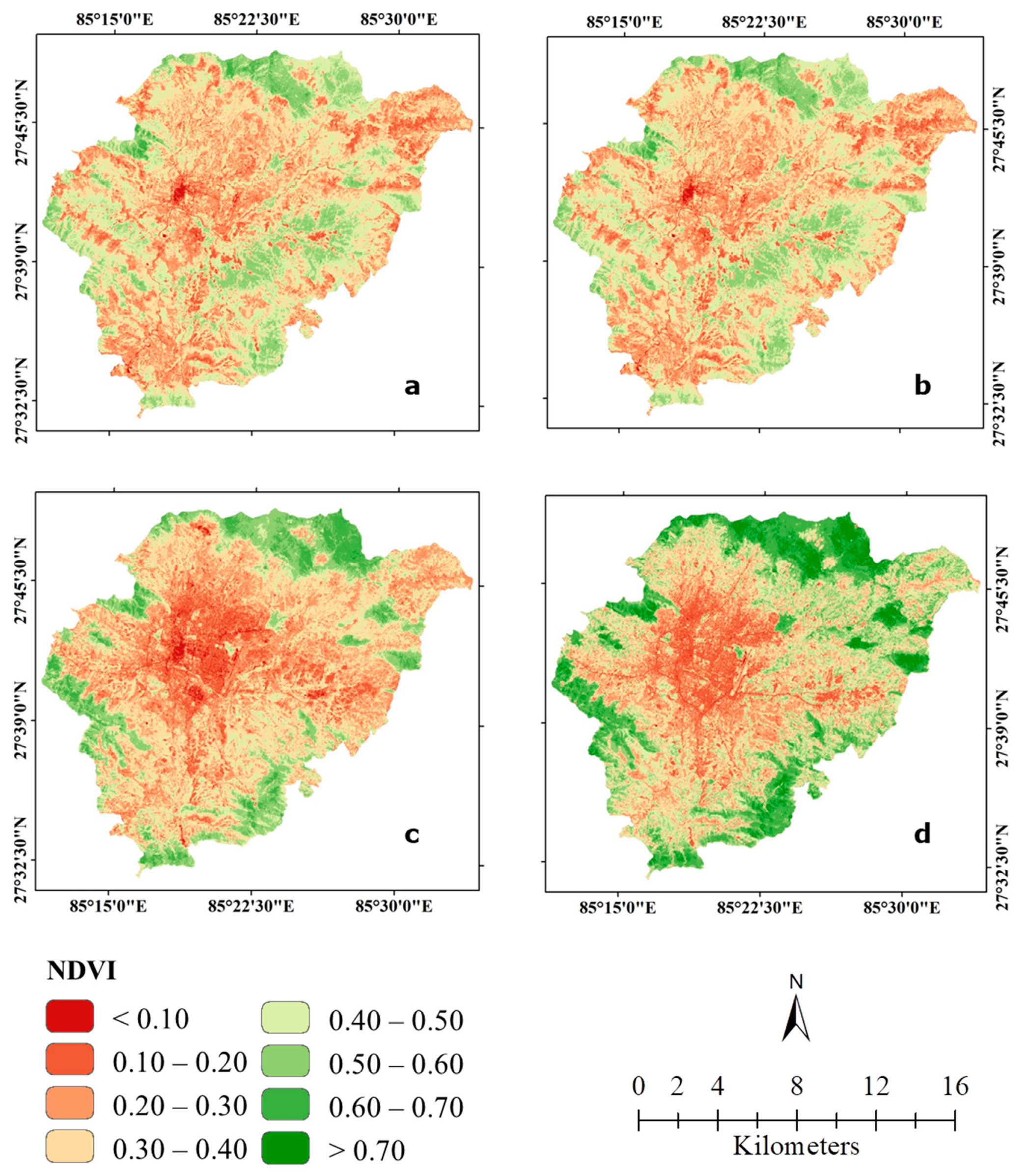
2.5. NDVI
2.6. NDBI
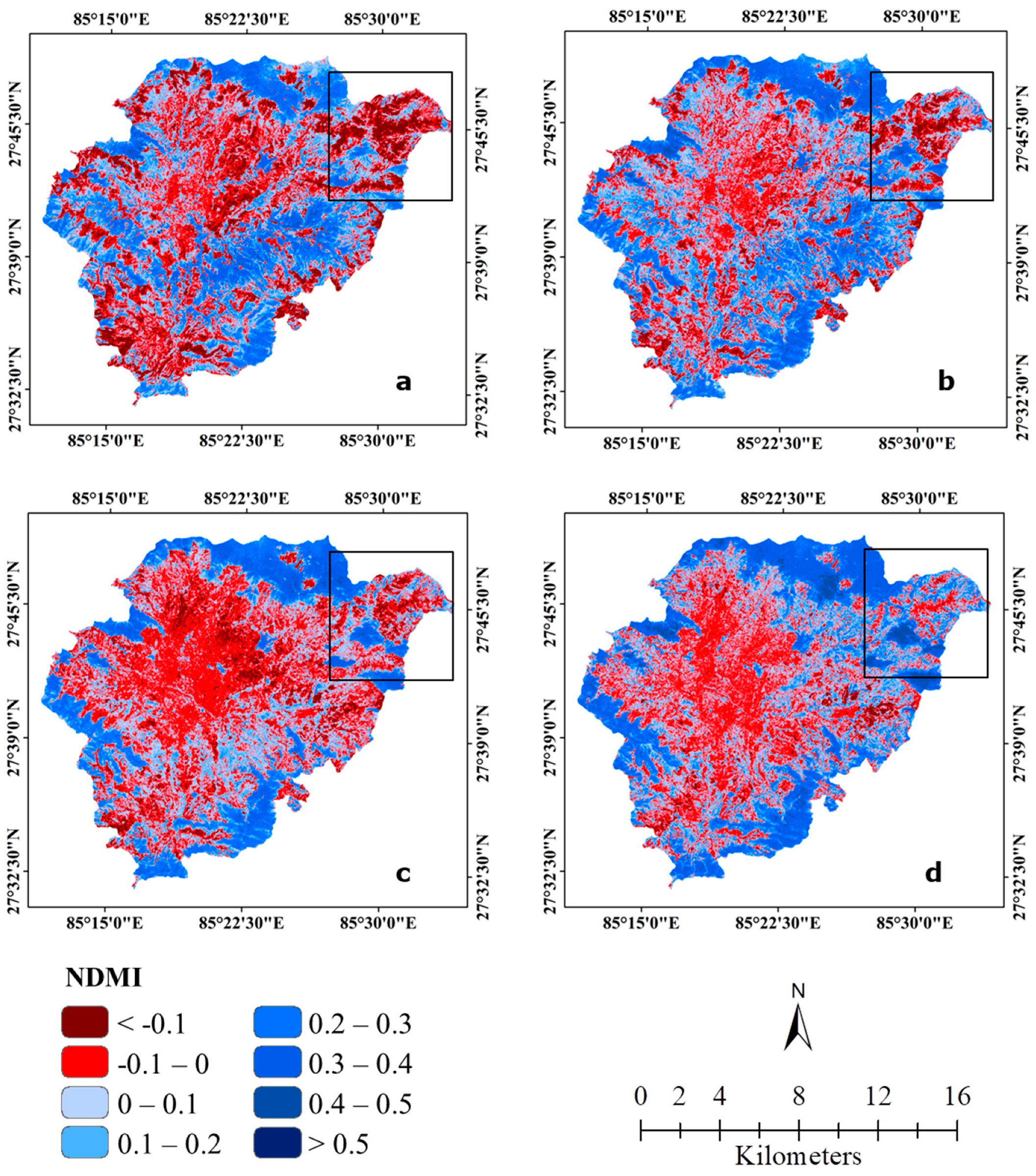
2.7. NDMI
2.8. Analysis of Urban–Rural Gradient
2.9. Statistical Analysis (Pearson’s Correlation Coefficient)
3. Results
3.1. Accuracy Assessment of LULC Classification
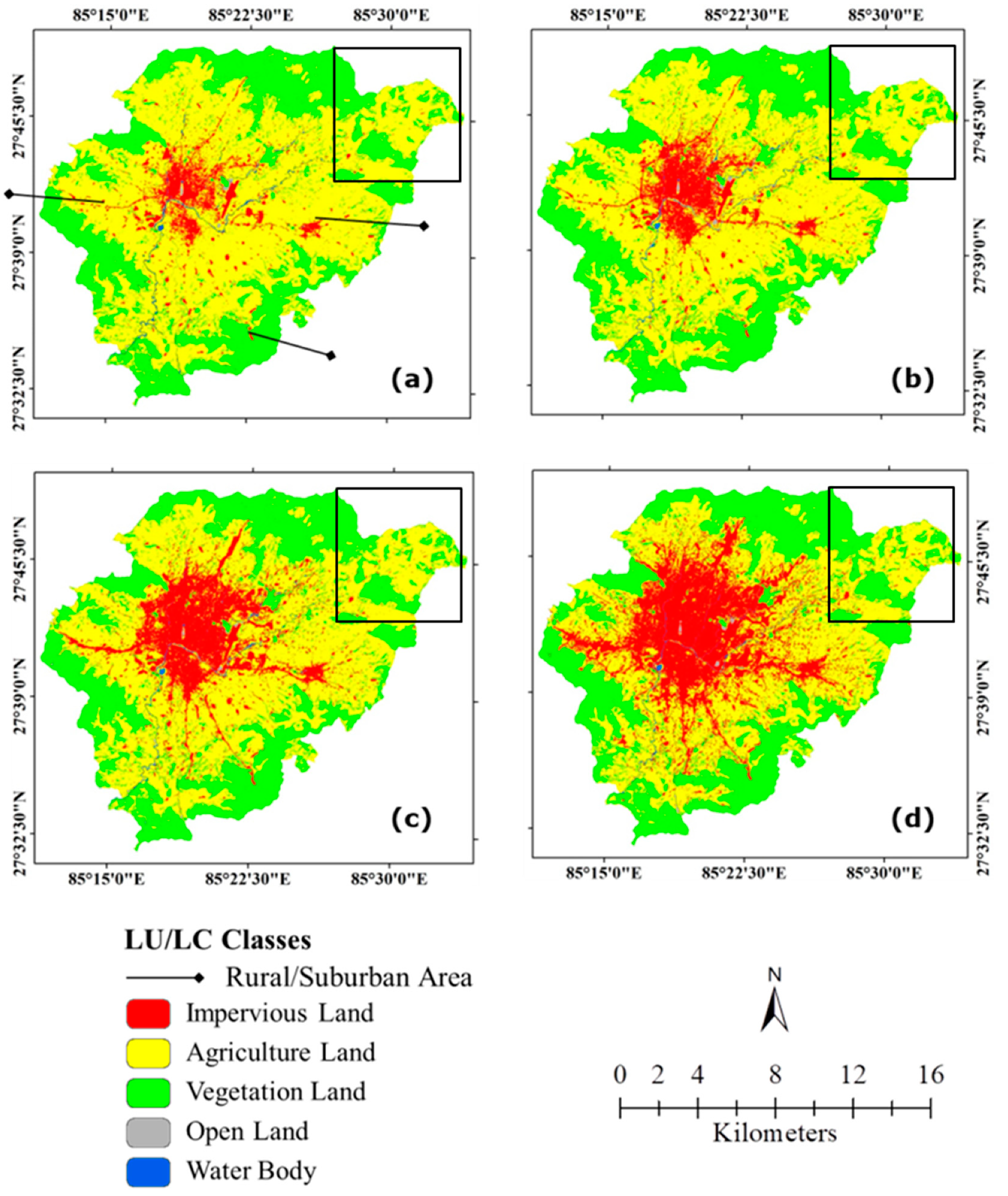
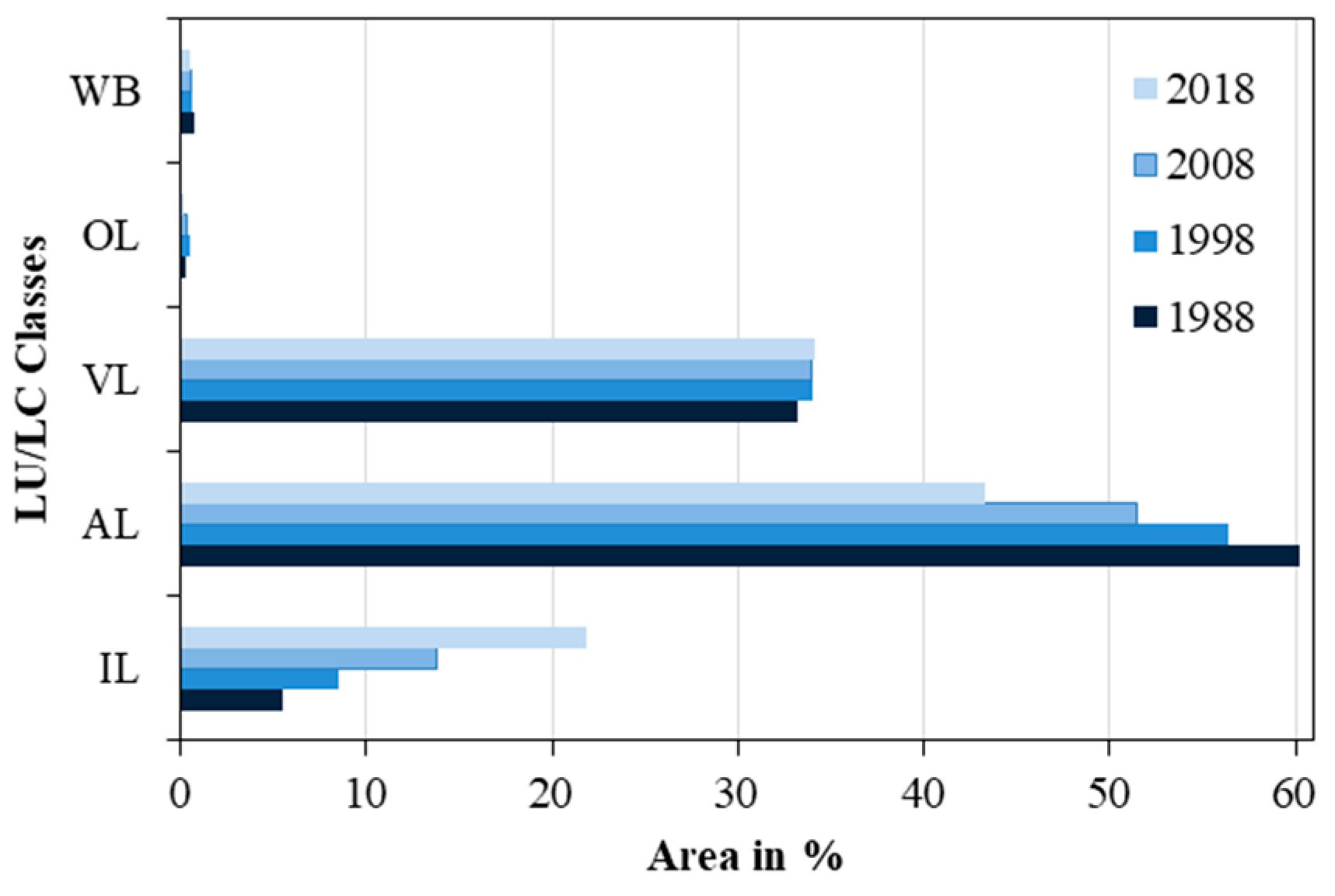
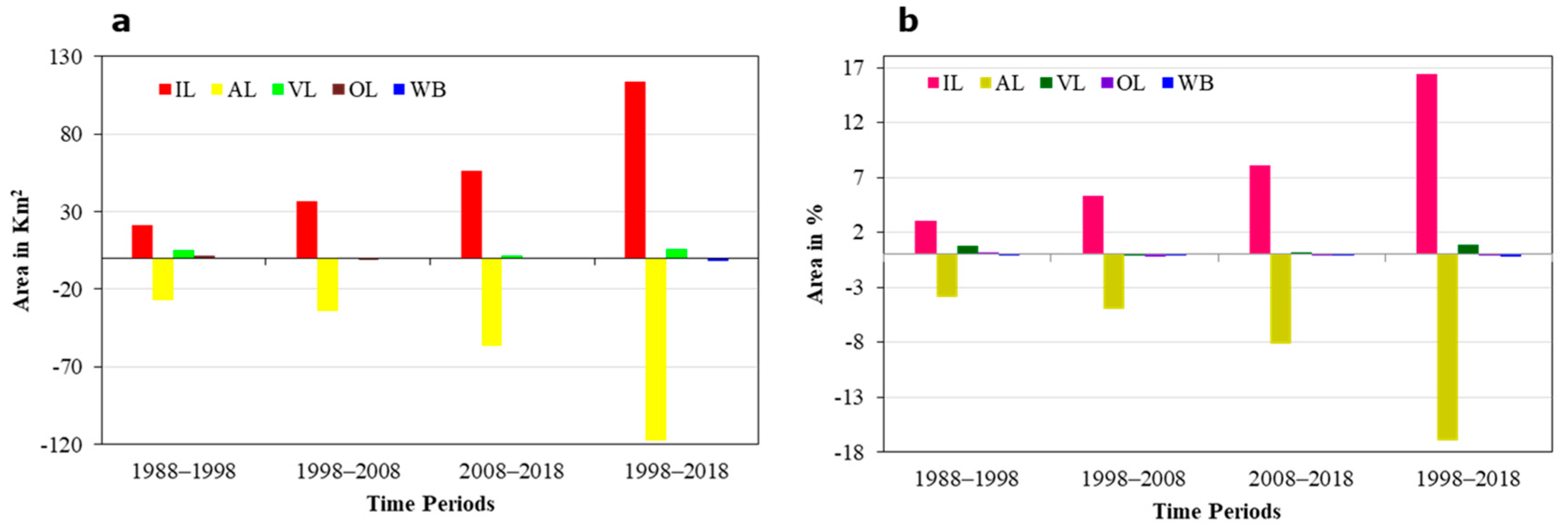
3.2. LULC Analysis
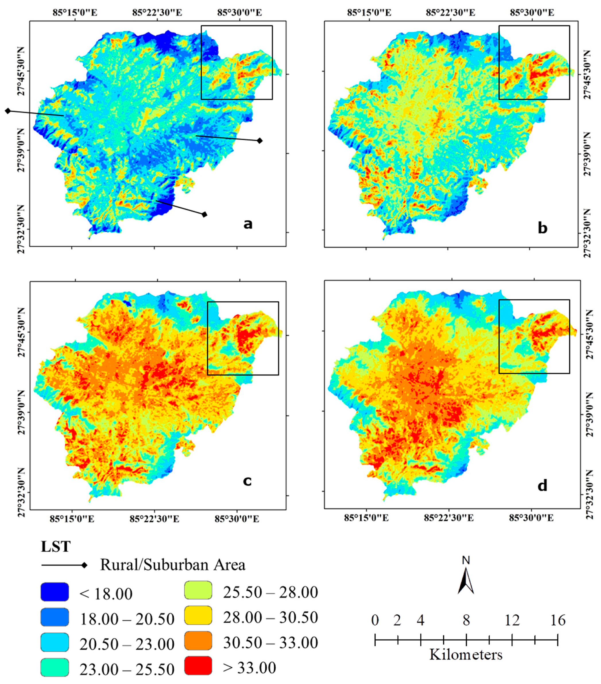
3.3. LST Analysis
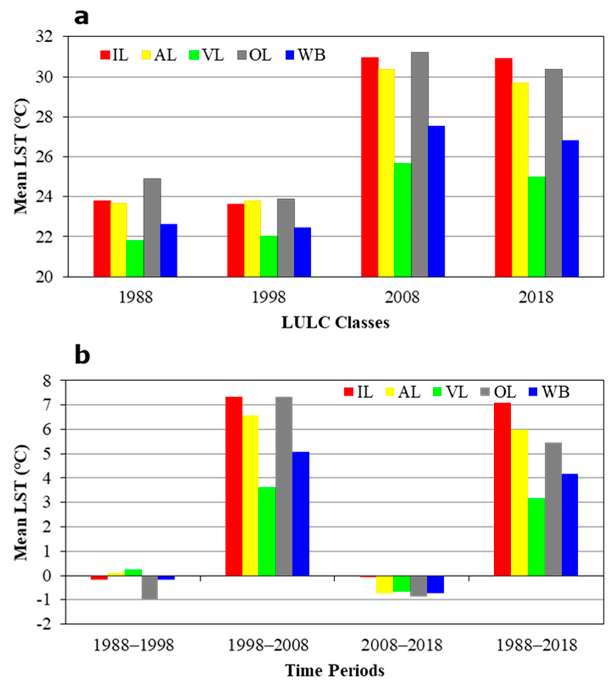
3.4. LULC Differences in LST
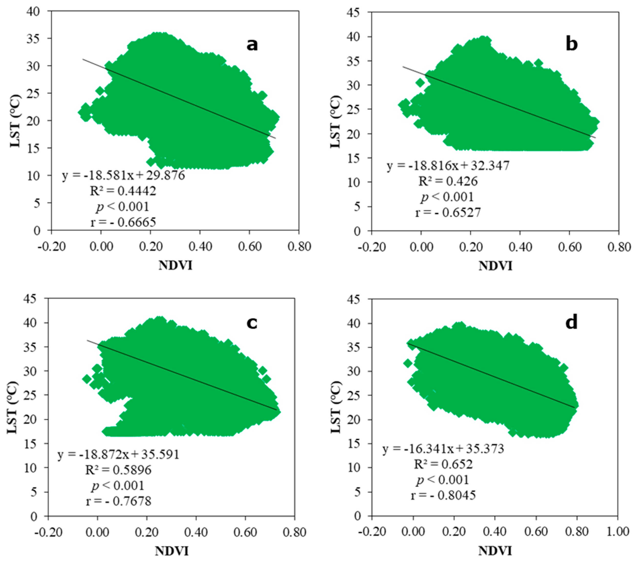
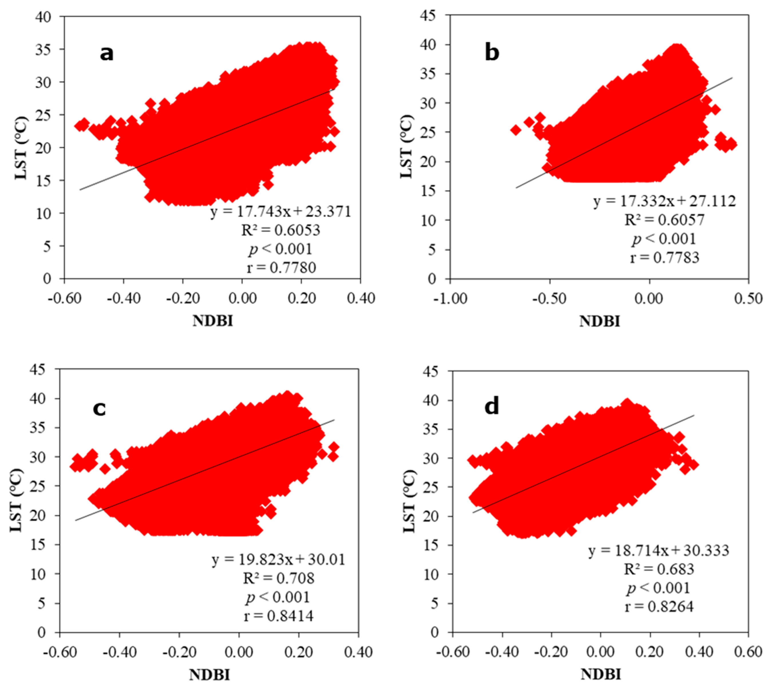
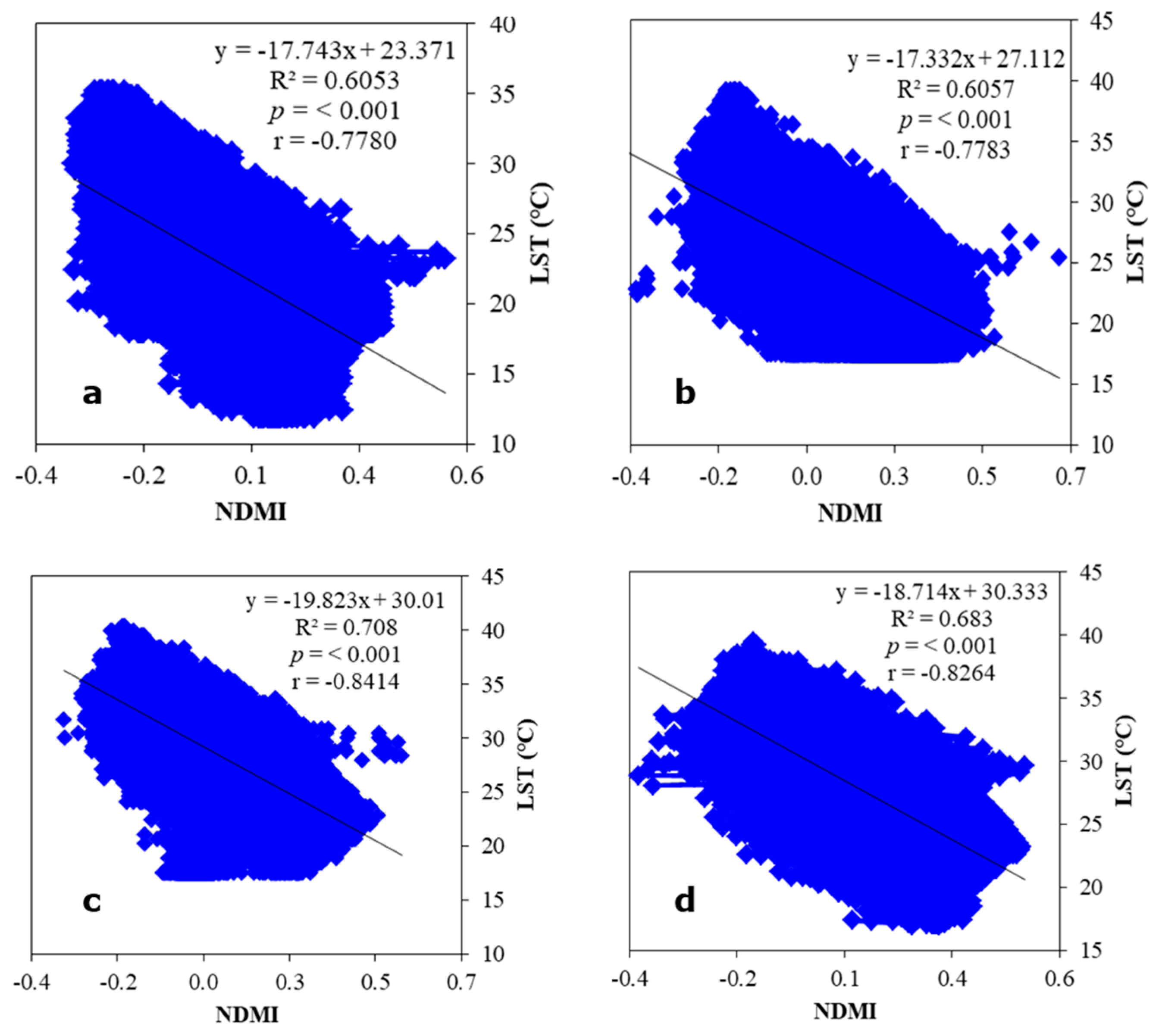
3.5. Spatiotemporal NDVI, NDBI, and NDMI Patterns and Their Influence on LST
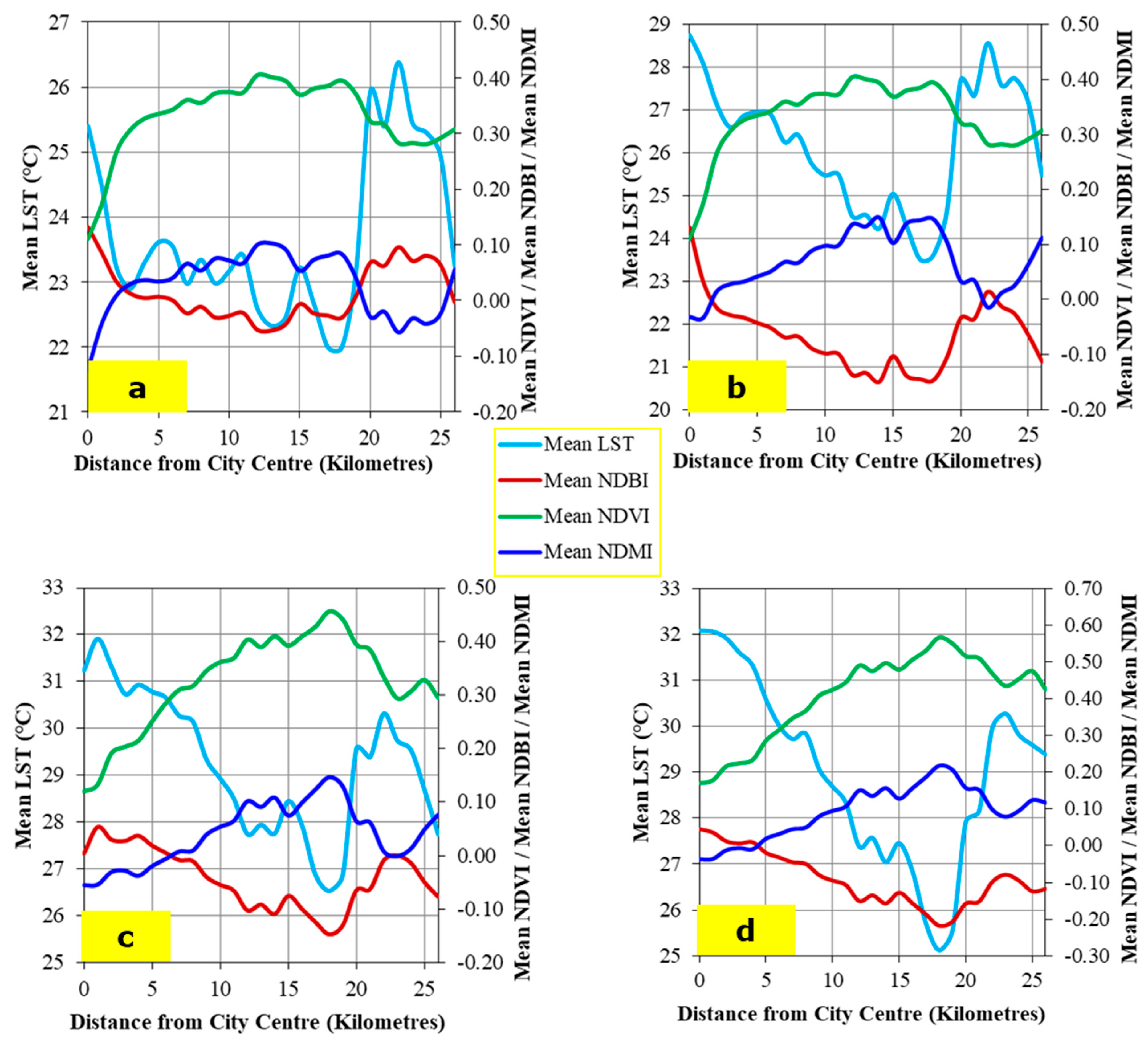
3.6. Analysis of Urban–Rural Gradient Pattern
4. Discussion
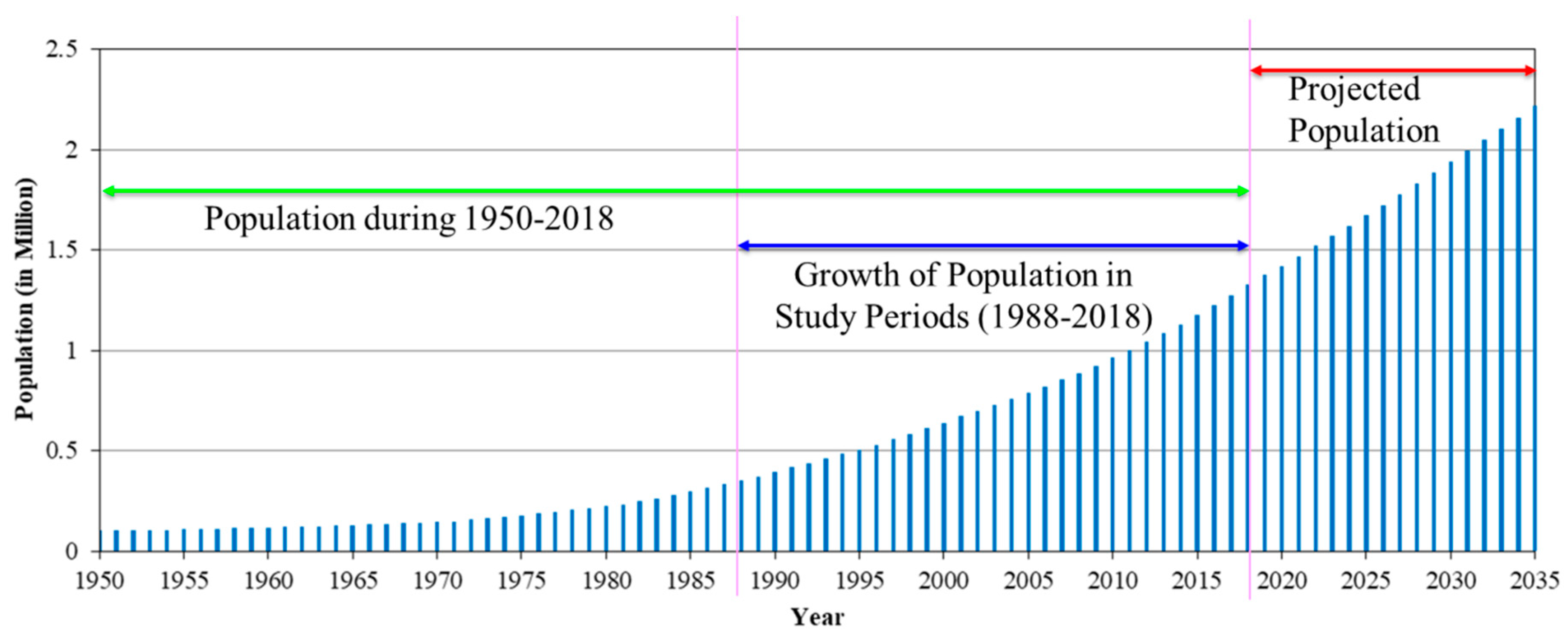
4.1. Urbanization from the Perspective of LULC Transformation and Population Explosion
4.2. Phenomena of SUHI and Sustainable Planning
4.3. Urban Sustainability Implication
5. Conclusions
Supplementary Materials
Author Contributions
Funding
Acknowledgments
Conflicts of Interest
Appendix A


| LULC Class | Year | ||||
|---|---|---|---|---|---|
| 1988 | 1998 | 2008 | 2018 | ||
| User Accuracy (%) | IL | 88.0 | 89.0 | 91.0 | 96.0 |
| AL | 95.5 | 96.0 | 96.5 | 96.0 | |
| VL | 84.5 | 90.0 | 95.5 | 96.5 | |
| OL | 93.5 | 94.0 | 95.0 | 96.0 | |
| WB | 97.5 | 98.0 | 96.5 | 98.5 | |
| Producer Accuracy (%) | IL | 92.6 | 87.3 | 94.8 | 93.7 |
| AL | 83.8 | 86.9 | 91.0 | 93.7 | |
| VL | 90.0 | 95.7 | 96.4 | 97.8 | |
| OL | 99.4 | 99.5 | 99.5 | 100 | |
| WB | 94.7 | 97.0 | 98.0 | 98.5 | |
| Overall Accuracy (%) | 95.2 | 93.4 | 95.2 | 96.6 | |
| Kappa Coefficient | 0.897 | 0.917 | 0.940 | 0.958 | |
| Year | LULC Classes | ||||||
|---|---|---|---|---|---|---|---|
| IL | AL | VL | OL | WB | Total | ||
| 1988 | Km2 | 37.98 | 418.32 | 230.69 | 1.97 | 5.31 | 694.27 |
| % | 5.47 | 60.25 | 33.23 | 0.28 | 0.76 | 100 | |
| 1998 | Km2 | 58.96 | 391.46 | 235.85 | 3.45 | 4.55 | 694.27 |
| % | 8.49 | 56.38 | 33.97 | 0.5 | 0.66 | 100 | |
| 2008 | Km2 | 95.45 | 356.63 | 235.4 | 3.34 | 3.45 | 694.27 |
| % | 13.75 | 51.37 | 33.91 | 0.48 | 0.5 | 100 | |
| 2018 | Km2 | 151.42 | 300.03 | 236.76 | 3.05 | 3.01 | 694.27 |
| % | 21.81 | 43.22 | 34.1 | 0.44 | 0.43 | 100 | |
| Year | LULC Type | |||||
|---|---|---|---|---|---|---|
| IL | AL | VL | OL | WB | ||
| 1988–1998 | Km2 | 20.99 | −26.86 | 5.16 | 1.48 | −0.76 |
| % | 3.02 | −3.87 | 0.74 | 0.22 | −0.1 | |
| 1998–2008 | Km2 | 36.49 | −34.83 | −0.47 | −0.11 | −1.1 |
| % | 5.26 | −5.01 | −0.06 | −0.02 | −0.16 | |
| 2008–2018 | Km2 | 55.97 | −56.6 | 1.38 | −0.3 | −0.44 |
| % | 8.06 | −8.15 | 0.19 | −0.04 | −0.07 | |
| 1988–2018 | Km2 | 113.44 | −118.29 | 6.07 | 1.07 | −2.3 |
| % | 16.34 | −17.03 | 0.87 | 0.16 | −0.33 | |
| Comparison of LULC Class | LULC Class (Cross Cover Comparison) | Mean LST Magnitude (°C) | |||
|---|---|---|---|---|---|
| 1988 | 1998 | 2008 | 2018 | ||
| IL vs. Other Class | IL-VL | 2.01 | 1.6 | 5.32 | 5.94 |
| IL-WB | 1.19 | 1.17 | 3.42 | 4.11 | |
| IL-AL | 0.12 | −0.17 | 0.59 | 1.25 | |
| IL-OL | −1.08 | −0.26 | −0.25 | 0.56 | |
| VL vs. Other Class | VL-IL | −2.01 | −1.6 | −5.32 | −5.94 |
| VL-AL | −1.89 | −1.77 | −4.73 | −4.69 | |
| VL-OL | −3.09 | −1.86 | −5.57 | −5.38 | |
| VL-WB | −0.82 | −0.43 | −1.9 | −1.83 | |
| WB vs. Other Class | WB-IL | −1.19 | −1.17 | −3.42 | −4.11 |
| WB-AL | −1.07 | −1.34 | −2.83 | −2.86 | |
| WB-VL | 0.82 | 0.43 | 1.9 | 1.83 | |
| WB-OL | −2.27 | −1.43 | −3.67 | −1.55 | |
References
- Feng, Y.; Du, S.; Myint, S.W.; Shu, M. Do urban functional zones affect land surface temperature differently? A case study of Beijing, China. Remote Sens. 2019, 11, 1802. [Google Scholar] [CrossRef] [Green Version]
- Ranagalage, M.; Wang, R.; Gunarathna, M.H.J.P.; Dissanayake, D.; Murayama, Y.; Simwanda, M. Spatial Forecasting of the Landscape in Rapidly Urbanizing Hill Stations of South Asia : A Case Study of Nuwara Eliya, Sri Lanka (1996–2037). Remote Sens. 2019, 11, 1743. [Google Scholar] [CrossRef] [Green Version]
- Shukla, A.; Jain, K. Modeling Urban Growth Trajectories and Spatiotemporal Pattern: A Case Study of Lucknow City, India. J. Indian Soc. Remote Sens. 2019, 47, 139–152. [Google Scholar] [CrossRef]
- UN Department of Economic and Social Affairs. Population Division. World Urbanization Prospects: The 2018 Revision. Online Edition. 2018. Available online: https://population.un.org/wup/ (accessed on 15 November 2020).
- Wang, C.; Myint, S.W.; Wang, Z.; Song, J. Spatio-Temporal Modeling of the Urban Heat Island in the Phoenix Metropolitan Area: Land Use Change Implications. Remote Sens. 2016, 8, 185. [Google Scholar] [CrossRef] [Green Version]
- Keeratikasikorn, C.; Bonafoni, S. Urban heat island analysis over the land use zoning plan of Bangkok by means of Landsat 8 imagery. Remote Sens. 2018, 10, 440. [Google Scholar] [CrossRef]
- IPCC Climate Change and Land. An IPCC Special Report on climate change, desertification, land degradation, sustainable land management, food security, and greenhouse gas fluxes in terrestrial ecosystems. In Summary for Policymakers. 2019. Available online: https://www.ipcc.ch/site/assets/uploads/sites/4/2020/02/SPM_Updated-Jan20.pdf (accessed on 15 November 2020).
- Weng, Q.; Lu, D.; Schubring, J. Estimation of land surface temperature-vegetation abundance relationship for urban heat island studies. Remote Sens. Environ. 2004, 89, 467–483. [Google Scholar] [CrossRef]
- Estoque, R.C.; Murayama, Y.; Myint, S.W. Effects of landscape composition and pattern on land surface temperature: An urban heat island study in the megacities of Southeast Asia. Sci. Total Environ. 2017, 577, 349–359. [Google Scholar] [CrossRef]
- Rousta, I.; Sarif, M.O.; Gupta, R.D.; Olafsson, H.; Ranagalage, M.; Murayama, Y.; Zhang, H.; Mushore, T.D. Spatiotemporal Analysis of Land Use/Land Cover and Its Effects on Surface Urban Heat Island Using Landsat Data : A Case Study of Metropolitan City Tehran (1988–2018). Sustainability 2018, 10, 4433. [Google Scholar] [CrossRef] [Green Version]
- Wang, R.; Derdouri, A.; Murayama, Y. Spatiotemporal simulation of future land use/cover change scenarios in the Tokyo metropolitan area. Sustainability 2018, 10, 2056. [Google Scholar] [CrossRef] [Green Version]
- Rimal, B.; Keshtkar, H.; Sharma, R.; Stork, N.; Rijal, S.; Kunwar, R. Simulating urban expansion in a rapidly changing landscape in eastern Tarai, Nepal. Environ. Monit. Assess. 2019, 191, 255. [Google Scholar] [CrossRef]
- Bokaie, M.; Zarkesh, M.K.; Arasteh, P.D.; Hosseini, A. Assessment of urban heat island based on the relationship between land surface temperature and land use/land cover in Tehran. Sustain. Cities Soc. 2016, 23, 94–104. [Google Scholar] [CrossRef]
- Son, N.T.; Chen, C.F.; Chen, C.R.; Thanh, B.X.; Vuong, T.H. Assessment of urbanization and urban heat islands in Ho Chi Minh city, Vietnam using Landsat data. Sustain. Cities Soc. 2017, 30, 150–161. [Google Scholar] [CrossRef]
- Babazadeh, M.; Kumar, P. Estimation of the urban heat island in local climate change and vulnerability assessment for air quality in Delhi. Eur. Sci. J. 2015, 1, 55–65. [Google Scholar]
- Stewart, I.D.; Oke, T.R. Local climate zones for urban temperature studies. Bull. Am. Meteorol. Soc. 2012, 93, 1879–1900. [Google Scholar] [CrossRef]
- Joshi, R.; Raval, H.; Pathak, M.; Prajapati, S.; Patel, A.; Singh, V.; Kalubarme, M.H. Urban heat island characterization and isotherm mapping using geo-informatics technology in Ahmedabad city, Gujarat state, India. Int. J. Geosci. 2015, 6, 274–285. [Google Scholar] [CrossRef] [Green Version]
- Rosa, A.; De Oliveira, F.S.; Gomes, A.; Gleriani, J.M.; Gonçalves, W.; Moreira, G.L.; Silva, F.G.; Ricardo, E.; Branco, F.; Moura, M.M.; et al. Spatial and temporal distribution of urban heat islands. Sci. Total Environ. 2017, 605–606, 946–956. [Google Scholar]
- Avdan, U.; Jovanovska, G. Algorithm for automated mapping of land surface temperature using Landsat 8 tatellite data. J. Sens. 2016, 2016, 1–8. [Google Scholar] [CrossRef] [Green Version]
- Li, X.; Zhou, Y.; Asrar, G.R.; Imhoff, M.; Li, X. The surface urban heat island response to urban expansion : A panel analysis for the conterminous United States. Sci. Total Environ. 2017, 605–606, 426–435. [Google Scholar] [CrossRef]
- Zhang, X.; Estoque, R.C.; Murayama, Y. An urban heat island study in Nanchang City, China based on land surface temperature and social-ecological variables. Sustain. Cities Soc. 2017, 32, 557–568. [Google Scholar] [CrossRef]
- Gagliano, A.; Detommaso, M.; Nocera, F.; Evola, G. A multi-criteria methodology for comparing the energy and environmental behavior of cool, green and traditional roofs. Build. Environ. 2015, 90, 71–81. [Google Scholar] [CrossRef]
- Chaudhuri, A.S.; Singh, P.; Rai, S.C. Modelling LULC change dynamics and its impact on environment and water security: Geospatial technology based assessment. Ecol. Environ. Conserv. 2018, 24, 300–306. [Google Scholar]
- Yao, R.; Wang, L.; Huang, X.; Guo, X.; Niu, Z.; Liu, H. Investigation of urbanization effects on land surface phenology in northeast China during 2001–2015. Remote Sens. 2017, 9, 66. [Google Scholar] [CrossRef] [Green Version]
- Dewan, A.M.; Yamaguchi, Y. Land use and land cover change in Greater Dhaka, Bangladesh: Using remote sensing to promote sustainable urbanization. Appl. Geogr. 2020, 29, 390–401. [Google Scholar] [CrossRef]
- Ramachandra, T.V.; Kumar, U. Land surface temperature with land cover dynamics: Multi-resolution, rpatio-temporal data analysis of Greater Bangalore. Int. J. Geoinform. 2009, 5, 43–53. [Google Scholar]
- Pandey, P.; Kumar, D.; Prakash, A.; Masih, J.; Singh, M.; Kumar, S.; Jain, V.K.; Kumar, K. Science of the Total Environment A study of urban heat island and its association with particulate matter during winter months over Delhi. Sci. Total Environ. 2012, 414, 494–507. [Google Scholar] [CrossRef]
- Ku, D.N.; Sandeep, N.; Jyothi, S.; Madhu, T. Significant changes on land use/land cover by using remote sensing and GIS analysis-review. Int. J. Eng. Sci. Comput. 2017, 7, 5433–5435. [Google Scholar]
- Gould, W.A.; Gonz, O.M.R. Land development, land use, and urban sprawl in Puerto Rico integrating remote sensing and population census data. Landsc. Urban Plan. 2007, 79, 288–297. [Google Scholar]
- Kuang, W.; Liu, Y.; Dou, Y.; Chi, W.; Chen, G. What are hot and what are not in an urban landscape : Quantifying and explaining the land surface temperature pattern in Beijing, China. Landsc. Ecol. 2015, 30, 357–373. [Google Scholar] [CrossRef]
- Zhang, Y.; Su, Z.; Li, G.; Zhuo, Y.; Xu, Z. Spatial-temporal evolution of sustainable urbanization development: A perspective of the coupling coordination development based on population, industry, and built-up land spatial agglomeration. Sustainability 2018, 10, 1766. [Google Scholar] [CrossRef] [Green Version]
- Sultana, S.; Satyanarayana, A.N.V. Urban heat island intensity during winter over metropolitan cities of India using remote-sensing techniques: Impact of urbanization. Int. J. Remote Sens. 2018, 39, 6692–6730. [Google Scholar] [CrossRef]
- Kumar, R.; Mishra, V.; Buzan, J.; Kumar, R.; Shindell, D.; Huber, M. Dominant control of agriculture and irrigation on urban heat island in India. Sci. Rep. 2017, 7, 14054. [Google Scholar] [CrossRef] [PubMed]
- Kumar, S.; Panwar, M. Urban heat island footprint mapping of Delhi using remote sensing. Int. J. Emerg. Technol. 2017, 8, 80–83. [Google Scholar]
- Agarwal, R.; Sharma, U.; Taxak, A. Remote sensing based assessment of urban heat island phenomenon in Nagpur metropolitan area. Int. J. Inf. Comput. Technol. 2014, 4, 1069–1074. [Google Scholar]
- Mukherjee, S.; Joshi, P.K.; Garg, R.D. Analysis of urban built-up areas and surface urban heat island using downscaled MODIS derived land surface temperature data. Geocarto Int. 2017, 32, 900–918. [Google Scholar] [CrossRef]
- Gunaalan, K.; Ranagalage, M.; Gunarathna, M.H.J.P.; Kumari, M.K.N.; Vithanage, M.; Srivaratharasan, T.; Saravanan, S.; Warnasuriya, T.W.S. Application of geospatial techniques for groundwater quality and availability assessment: A case study in Jaffna Peninsula, Sri Lanka. ISPRS Int. J. Geo-Inf. 2018, 7, 20. [Google Scholar] [CrossRef] [Green Version]
- Pal, S.; Ziaul, S. Detection of land use and land cover change and land surface temperature in English Bazar urban centre. Egypt. J. Remote Sens. Sp. Sci. 2017, 20, 125–145. [Google Scholar] [CrossRef] [Green Version]
- Renard, F.; Alonso, L.; Fitts, Y.; Hadjiosif, A.; Comby, J. Evaluation of the Effect of Urban Redevelopment on Surface Urban Heat Islands. Remote Sens. 2019, 11, 1–31. [Google Scholar] [CrossRef] [Green Version]
- Thapa, R.B.; Murayama, Y. Drivers of urban growth in the Kathmandu valley, Nepal: Examining the efficacy of the analytic hierarchy process. Appl. Geogr. 2010, 30, 70–83. [Google Scholar] [CrossRef]
- Estoque, R.C.; Pontius, R.G.; Murayama, Y.; Hou, H.; Thapa, R.B.; Lasco, R.D.; Villar, M.A. Simultaneous comparison and assessment of eight remotely sensed maps of Philippine forests. Int. J. Appl. Earth Obs. Geoinf. 2018, 67, 123–134. [Google Scholar] [CrossRef]
- Toffin, G. Urban fringes: Squatter and slum settlements in the Kathmandu Valley (Nepal). Contrib. Nepal. Stud. 2010, 37, 151–168. [Google Scholar]
- Thapa, R.B.; Murayama, Y. Examining Spatiotemporal Urbanization Patterns in Kathmandu Valley, Nepal: Remote Sensing and Spatial Metrics Approaches. Remote Sens. 2009, 1, 534–556. [Google Scholar] [CrossRef] [Green Version]
- Chitrakar, R.M.; Baker, D.C.; Guaralda, M. Urban growth and development of contemporary neighbourhood public space in Kathmandu Valley, Nepal. Habitat Int. 2016, 53, 30–38. [Google Scholar] [CrossRef] [Green Version]
- Rimal, B.; Zhang, L.; Keshtkar, H.; Wang, N.; Lin, Y. Monitoring and modeling of spatiotemporal urban expansion and Land-Use/Land-Cover change using integrated Markov Chain Cellular Automata Model. ISPRS Int. J. Geo-Inf. 2017, 6, 288. [Google Scholar] [CrossRef] [Green Version]
- Rimal, B.; Zhang, L.; Keshtkar, H.; Barry, N.H.; Rijal, S.; Zhang, P. Land Use/Land Cover Dynamics and Modeling of Urban Land Expansion by the Integration of Cellular Automata and Markov Chain. ISPRS Int. J. Geo-Inf. 2018, 7, 154. [Google Scholar] [CrossRef] [Green Version]
- Ishtiaque, A.; Shrestha, M.; Chhetri, N. Rapid urban growth in the Kathmandu valley, Nepal: Monitoring land use land cover dynamics of a himalayan city with Landsat imageries. Environments 2017, 4, 72. [Google Scholar] [CrossRef]
- Ranagalage, M.; Dmslb, D.; Murayama, Y.; Zhang, X.; Estoque, R.C.; Enc, P.; Morimoto, T. Quantifying surface urban heat island formation in the world heritage tropical mountain city of Sri Lanka. ISPRS Int. J. Geo-Inf. 2018, 7, 341. [Google Scholar] [CrossRef] [Green Version]
- NPSC National Population and Housing Census 2011 (Population Projection 2011–2031); Central Bureau of Statistics, Government of Nepal: Kathmandu, Nepal, 2014; Volume 8.
- Kottek, M.; Grieser, J.; Beck, C.; Rudolf, B.; Rubel, F. World Maps of Köppen-Geiger Climate Classification. Meteorol. Z. 2006, 15, 259–263. [Google Scholar] [CrossRef]
- MoLRM Topographical Map; Ministry of Land Ressources and Management Survey Department, Topographic Survey Branch (Ed.) Min Bhawan: Kathmandu, Nepal, 1995. [Google Scholar]
- Talukdar, S.; Singha, P.; Mahato, S.; Pal, S.; Liou, Y.; Rahman, A. Land-Use Land-Cover Classification by Machine Learning Classifiers for Satellite Observations—A Review. Remote Sens. 2020, 12, 1135. [Google Scholar] [CrossRef] [Green Version]
- Rimal, B.; Zhang, L.; Keshtkar, H.; Huejian, S.; Rijal, S. Quantifying the Spatiotemporal Pattern of Urban Expansion and Hazard and Risk Area Identification in the Kaski District of Nepal. Land 2018, 7, 37. [Google Scholar] [CrossRef] [Green Version]
- Rimal, B.; Rijal, S.; Kunwar, R. Comparing Support Vector Machines and Maximum Likelihood Classifiers for Mapping of Urbanization. J. Indian Soc. Remote Sens. 2020, 48, 71–79. [Google Scholar] [CrossRef]
- Schneider, A. Monitoring land cover change in urban and peri-urban areas using dense time stacks of Landsat satellite data and a data mining approach. Remote Sens. Environ. 2012, 124, 689–704. [Google Scholar] [CrossRef]
- Lee, S.; Hong, S.M.; Jung, H.S. A support vector machine for landslide susceptibility mapping in Gangwon Province, Korea. Sustainability 2017, 9, 48. [Google Scholar] [CrossRef] [Green Version]
- Pervez, W.; Uddin, V.; Khan, S.A.; Khan, J.A. Satellite-based land use mapping: Comparative analysis of Landsat-8, Advanced Land Imager, and big data Hyperion imagery. J. Appl. Remote Sens. 2019, 10, 026004. [Google Scholar] [CrossRef] [Green Version]
- Anderson, J.R.; Hardy, E.E.; Roach, J.T.; Witmer, R.E.; Anderson, J.R.; Hardy, E.E.; Roach, J.T.; Witmer, R.E. A Land Use And Land Cover Classification System For Use With Remote Sensor Data. In A Rezvision of the Land Use Classification System as presented in U.S. Geological Survey Circular 671; United States Government Printing Office: Washington, DC, USA, 1976. [Google Scholar]
- Jensen, J.R. Introductory Digital Image Processing A Remote Sensing Perspective Second Edition; Pearson: Hoboken, NJ, USA, 1995; ISBN 978-0-13-205840-7. [Google Scholar]
- Roy, P.S.; Roy, A.; Joshi, P.K.; Kale, M.P.; Srivastava, V.K.; Srivastava, S.K.; Dwevidi, R.S.; Joshi, C.; Behera, M.D.; Meiyappan, P.; et al. Development of decadal (1985-1995-2005) land use and land cover database for India. Remote Sens. 2015, 7, 2401–2430. [Google Scholar] [CrossRef] [Green Version]
- Ziaul, S.; Pal, S. Suitability assessment for selecting new sites for installing water service centres within English Bazar Municipality, Malda, West Bengal. J. Settlements Spat. Plan. 2016, 7. [Google Scholar] [CrossRef]
- Nimish, G.; Bharath, H.A.; Lalitha, A. Exploring temperature indices by deriving relationship between land surface temperature and urban landscape Remote Sensing Applications: Society and Environment Exploring temperature indices by deriving relationship between land surface temperature and u. Remote Sens. Appl. Soc. Environ. 2020, 18, 100299. [Google Scholar]
- Sarif, M.O.; Gupta, R.D. Land Surface Temperature Profiling and its relationships with Land Indices: A case study on Lucknow City. In Proceedings of the ISPRS Annals of Photogrammetry, Remote Sensing and Spatial Information Sciences; Copernicus Publications: Göttingen, Germany, 2019; Volume IV-5/W2, pp. 89–96. [Google Scholar]
- Sobrino, J.A.; Jiménez-Muñoz, J.C.; Paolini, L. Land surface temperature retrieval from LANDSAT TM 5. Remote Sens. Environ. 2004, 90, 434–440. [Google Scholar] [CrossRef]
- Sekertekin, A.; Bonafoni, S. Land Surface Temperature Retrieval from Landsat 5, 7, and 8 over Rural Areas: Assessment of Di ff erent Retrieval Algorithms and Emissivity Models and Toolbox Implementation. Remote Sens. 2020, 12, 294. [Google Scholar] [CrossRef] [Green Version]
- Skokovic, D.; Sobrino, J.A.; Jimenez-Munoz, J.C.; Soria, G.; Julien, Y.; Mattar, C.; Cristobal, J. Calibration and Validation of land surface temperature for landsat 8 TIRS sensor. In Proceedings of the Land Product Validation and Evolution; ESA/ESRIN: Frascati, Italy, 2014; pp. 1–27. [Google Scholar]
- USGS LANDSAT 8 (L8) DATA USERS HANDBOOK Version 1.0 June 2015. Dep. Inter. U. S. Geol. Surv. 2015, 8. Available online: https://prd-wret.s3-us-west-2.amazonaws.com/assets/palladium/production/atoms/files/LSDS-1574_L8_Data_Users_Handbook-v5.0.pdf (accessed on 15 November 2020).
- Ranagalage, M.; Estoque, R.C.; Murayama, Y. An urban heat island study of the Colombo metropolitan area, Sri Lanka, based on Landsat data (1997–2017). ISPRS Int. J. Geo-Inf. 2017, 6, 189. [Google Scholar] [CrossRef] [Green Version]
- Roshan, G.; Rousta, I.; Ramesh, M. Studying the effects of urban sprawl of metropolis on tourism-climate index oscillation: A case study of Tehran city. J. Geogr. Reg. Plan. 2009, 2, 310–321. [Google Scholar]
- Li, D.; Sun, T.; Liu, M.; Yang, L.; Wang, L.; Gao, Z. Contrasting responses of urban and rural surface energy budgets to heat waves explain synergies between urban heat islands and heat waves. Environ. Res. Lett. 2015, 10, 054009. [Google Scholar] [CrossRef]
- Padmanaban, R.; Bhowmik, A.K.; Cabral, P.; Zamyatin, A.; Almegdadi, O.; Wang, S. Modelling urban sprawl using remotely sensed data: A case study of Chennai city, Tamilnadu. Entropy 2017, 19, 163. [Google Scholar] [CrossRef] [Green Version]
- Singh, P.; Kikon, N.; Verma, P. Impact of land use change and urbanization on urban heat island in Lucknow city, Central India: A remote sensing based estimate. Sustain. Cities Soc. 2017, 32, 100–114. [Google Scholar] [CrossRef]
- Pathak, C.; Chandra, S.; Maurya, G.; Rathore, A.; Sarif, M.O.; Gupta, R.D. The Effects of Land Indices on Thermal State in Surface Urban Heat Island Formation: A Case Study on Agra City in India Using Remote Sensing Data (1992–2019). Earth Syst. Environ. 2020. [Google Scholar] [CrossRef]
- Xi, Y.; Thinh, N.X.; Li, C. Spatio-Temporal Variation Analysis of Landscape Pattern Response to Land Use Change from 1985 to 2015 in Xuzhou City, China. Sustainability 2018, 10, 4287. [Google Scholar] [CrossRef] [Green Version]
- Estoque, R.C.; Murayama, Y. Monitoring surface urban heat island formation in a tropical mountain city using Landsat data (1987–2015). ISPRS J. Photogramm. Remote Sens. 2017, 133, 18–29. [Google Scholar] [CrossRef]
- Nigussie, T.A.; Altunkaynak, A.; Asce, A.M. Modeling urbanization of Istanbul under different scenarios using SLEUTH urban growth model. J. Urban Plan. Dev. 2016, 1–13. [Google Scholar] [CrossRef]
- Krajewski, P. Assessing change in a high-value landscape: Case study of the municipality of Sobotka, Poland. Polish J. Environ. Stud. 2017, 26, 2603–2610. [Google Scholar] [CrossRef]
- García-Ayllón, S. Rapid development as a factor of imbalance in urban growth of cities in Latin America: A perspective based on territorial indicators. Habitat Int. 2016, 58, 127–142. [Google Scholar] [CrossRef]
- Fenta, A.A.; Yasuda, H.; Haregeweyn, N.; Belay, S.; Hadush, Z.; Gebremedhin, M.A. The dynamics of urban expansion and land use / land cover changes using remote sensing and spatial metrics: The case of Mekelle City of northern Ethiopia changes using remote sensing and spatial metrics: The case of Mekelle City of northern Ethiopia. Int. J. Remote Sens. 2017, 38, 4107–4129. [Google Scholar] [CrossRef]
- Garcia-Ayllon, S. Urban transformations as indicators of economic change in post-communist Eastern Europe: Territorial diagnosis through five case studies. Habitat Int. 2018, 71, 29–37. [Google Scholar] [CrossRef]
- Ogashawara, I.; da Bastos, V.S.B. A Quantitative Approach for Analyzing the Relationship between Urban Heat Islands and Land Cover. Remote Sens. 2012, 4, 3596–3618. [Google Scholar] [CrossRef] [Green Version]
- Mohajerani, A.; Bakaric, J.; Jeffrey-Bailey, T. The urban heat island effect, its causes, and mitigation, with reference to the thermal properties of asphalt concrete. J. Environ. Manag. 2017, 197, 522–538. [Google Scholar] [CrossRef]
- Sen, S.; Roesler, J.; Ruddell, B.; Middel, A. Cool Pavement Strategies for Urban Heat Island Mitigation in Suburban Phoenix, Arizona. Sustainability 2019, 11, 4452. [Google Scholar] [CrossRef] [Green Version]
- Rimal, B.; Sloan, S.; Keshtkar, H.; Sharma, R.; Rijal, S.; Shrestha, U.B. Patterns of historical and future urban expansion in Nepal. Remote Sens. 2020, 12, 628. [Google Scholar] [CrossRef] [Green Version]
- Ranagalage, M.; Estoque, R.C.; Handayani, H.H.; Zhang, X.; Morimoto, T.; Tadono, T.; Murayama, Y. Relation between urban volume and land surface temperature: A comparative study of planned and traditional cities in Japan. Sustainability 2018, 10, 2366. [Google Scholar] [CrossRef] [Green Version]
- Dissanayake, D.; Morimoto, T.; Murayama, Y.; Ranagalage, M. Impact of Landscape Structure on the Variation of Land Surface Temperature in Sub-Saharan Region: A Case Study of Addis Ababa using Landsat Data. Sustainability 2019, 11, 2257. [Google Scholar] [CrossRef] [Green Version]


| Sensor | Path/Row | Resolution | Acquisition Date | Time (GMT) | Constants of Thermal Conversion | Source | |
|---|---|---|---|---|---|---|---|
| Landsat-5 TM | 141/41 | 30 m | 3 April 1988 | 04:18:24 | 607.76 (Band 6) | 1260.56 (Band 6) | United States Geological Survey (USGS) web portal (https://earthexplorer.usgs.gov/) |
| 15 April 1998 | 04:25:19 | 607.76 (Band 6) | 1260.56 (Band 6) | ||||
| 26 April 2008 | 04:37:22 | 607.76 (Band 6) | 1260.56 (Band 6) | ||||
| Landsat-8 OLI/TIRS | 22 April 2018 | 04:47:35 | 774.8853 (Band 10) | 1321.0789 (Band 10) | |||
| ASTER | - | 17 October 2011 | - | - | - | ||
| Date | Minimum (°C) | Maximum (°C) | Mean (°C) | Standard Deviation |
|---|---|---|---|---|
| 3 April 1988 | 11.88 | 35.25 | 23.08 | 3.09 |
| 15 April 1998 | 17.93 | 39.15 | 25.46 | 3.20 |
| 26 April 2008 | 17.47 | 40.30 | 28.86 | 3.31 |
| 22 April 2018 | 16.96 | 39.46 | 28.35 | 3.40 |
| The Mean LST difference in different time periods (°C) | ||||
| 1988–1998 | 1998–2008 | 2008–2018 | 1988–2018 | |
| 2.38 | 3.4 | −0.51 | 5.27 | |
| LULC Class | Mean LST (°C) | The Difference of Mean LST (°C) | ||||||
|---|---|---|---|---|---|---|---|---|
| 1988 | 1998 | 2008 | 2018 | 1988–1998 | 1998–2008 | 2008–2018 | 1988–2018 | |
| Impervious Land | 23.81 | 23.63 | 30.97 | 30.92 | −0.18 | 7.34 | −0.05 | 7.11 |
| Agriculture Land | 23.69 | 23.80 | 30.38 | 29.67 | 0.11 | 6.58 | −0.71 | 5.98 |
| Vegetation Land | 21.80 | 22.03 | 25.65 | 24.98 | 0.23 | 3.62 | −0.67 | 3.18 |
| Open Land | 24.89 | 23.89 | 31.22 | 30.36 | −1 | 7.33 | −0.86 | 5.47 |
| Water Body | 22.62 | 22.46 | 27.55 | 26.81 | −0.16 | 5.09 | −0.74 | 4.19 |
| Date | Statistics of NDVI and NDBI | Correlation with LST | |||||
|---|---|---|---|---|---|---|---|
| Minimum | Maximum | Mean | Standard Deviation | Correlation Coefficient | Significance (p) | ||
| 3 April 1988 | NDVI | −0.073 | 0.704 | 0.365 | 0.111 | −0.6665 | p < 0.001 |
| NDBI | −0.549 | 0.313 | −0.017 | 0.136 | 0.7780 | p < 0.001 | |
| NDMI | −0.313 | 0.549 | 0.017 | 0.136 | −0.7780 | p < 0.001 | |
| 15 April 1998 | NDVI | −0.074 | 0.704 | 0.367 | 0.111 | −0.6527 | p < 0.001 |
| NDBI | −0.671 | 0.416 | −0.095 | 0.144 | 0.7783 | p < 0.001 | |
| NDMI | −0.416 | 0.671 | 0.095 | 0.144 | −0.7783 | p < 0.001 | |
| 26 April 2008 | NDVI | −0.042 | 0.725 | 0.356 | 0.135 | −0.7678 | p < 0.001 |
| NDBI | −0.549 | 0.318 | −0.058 | 0.141 | 0.8414 | p < 0.001 | |
| NDMI | −0.318 | 0.549 | 0.058 | 0.141 | −0.8414 | p < 0.001 | |
| 22 April 2018 | NDVI | −0.025 | 0.787 | 0.430 | 0.168 | −0.8045 | p < 0.001 |
| NDBI | −0.519 | 0.378 | −0.106 | 0.150 | 0.8264 | p < 0.001 | |
| NDMI | −0.378 | 0.519 | 0.106 | 0.150 | −0.8264 | p < 0.001 | |
Publisher’s Note: MDPI stays neutral with regard to jurisdictional claims in published maps and institutional affiliations. |
© 2020 by the authors. Licensee MDPI, Basel, Switzerland. This article is an open access article distributed under the terms and conditions of the Creative Commons Attribution (CC BY) license (http://creativecommons.org/licenses/by/4.0/).
Share and Cite
Sarif, M.O.; Rimal, B.; Stork, N.E. Assessment of Changes in Land Use/Land Cover and Land Surface Temperatures and Their Impact on Surface Urban Heat Island Phenomena in the Kathmandu Valley (1988–2018). ISPRS Int. J. Geo-Inf. 2020, 9, 726. https://0-doi-org.brum.beds.ac.uk/10.3390/ijgi9120726
Sarif MO, Rimal B, Stork NE. Assessment of Changes in Land Use/Land Cover and Land Surface Temperatures and Their Impact on Surface Urban Heat Island Phenomena in the Kathmandu Valley (1988–2018). ISPRS International Journal of Geo-Information. 2020; 9(12):726. https://0-doi-org.brum.beds.ac.uk/10.3390/ijgi9120726
Chicago/Turabian StyleSarif, Md. Omar, Bhagawat Rimal, and Nigel E. Stork. 2020. "Assessment of Changes in Land Use/Land Cover and Land Surface Temperatures and Their Impact on Surface Urban Heat Island Phenomena in the Kathmandu Valley (1988–2018)" ISPRS International Journal of Geo-Information 9, no. 12: 726. https://0-doi-org.brum.beds.ac.uk/10.3390/ijgi9120726