DEM Void Filling Based on Context Attention Generation Model

1
College of Geomatics, Xi’an University of Science and Technology, Xi’an 710054, China
2
Schools of Remote Sensing and Information Engineering, Wuhan University, Wuhan 430079, China
*
Author to whom correspondence should be addressed.
ISPRS Int. J. Geo-Inf. 2020, 9(12), 734; https://0-doi-org.brum.beds.ac.uk/10.3390/ijgi9120734
Submission received: 15 September 2020
/
Revised: 26 November 2020
/
Accepted: 5 December 2020
/
Published: 7 December 2020
Abstract
:The digital elevation model (DEM) generates a digital simulation of ground terrain in a certain range with the usage of 3D point cloud data. It is an important source of spatial modeling information. Due to various reasons, however, the generated DEM has data holes. Based on the algorithm of deep learning, this paper aims to train a deep generation model (DGM) to complete the DEM void filling task. A certain amount of DEM data and a randomly generated mask are taken as network inputs, along which the reconstruction loss and generative adversarial network (GAN) loss are used to assist network training, so as to perceive the overall known elevation information, in combination with the contextual attention layer, and generate data with reliability to fill the void areas. The experimental results have managed to show that this method has good feature expression and reconstruction accuracy in DEM void filling, which has been proven to be better than that illustrated by the traditional interpolation method.
1. Introduction
The digital elevation model (DEM) has wide applications and significant value in surveying and mapping [1], hydrology [2] and earth science [3]. As of now, the common way to obtain DEM data is by low-altitude photogrammetry, in which the point cloud data is obtained by dense matching. By covering a large scope of areas, this method can provide image texture information so as to basically meet the requirement of DEM construction [4]. However, due to a series of reasons, such as the dead angle of aerial photography, matching deviation and insufficient point position, the DEM constructed in most circumstances has holes of different sizes and shapes. The DEM data with holes hinders the acquisition of various terrain and geomorphic structure information, which would further make it difficult to provide and couple geospatial information well. For example, in the process of actual production, if the constructed high spatial resolution DEM has voids, it will produce an incomplete expression of the morphological characteristics of erosion trenches [5], while the missing data would also easily cause erroneous estimation of the material balance accuracy of mountain glaciers [6] and difficulties in eliminating topographic cracks [7].
For those reasons, a large number of related studies have been carried out by scholars, both at home and abroad. The literature [8] uses the inverse distance weight method (IDW), local polynomial interpolation method (LPI), spline with tension method (ST) and other algorithms to interpolate the elevation sampling points, construct the DEM and obtain both the advantages and disadvantages of the above methods through comparative analyses. The extraction and interpolation functions of fractal simulation parameters were improved in [9], but despite that, the method would nonetheless have great limitations in correcting DEM errors caused by two-phase unwrapping. The literature [10] realized triangle network reconstruction without prior knowledge by calculating the Delaunay neighborhood projection of each data neighborhood point on the tangent plane of the point. However, the results of the above two methods depend on the sparsity and uniformity of the sampling points, while the algorithm is highly disturbed by known data. A radial basis function was originally used to interpolate scattered data [11]. The function and its improved form [12,13,14,15] were proposed, which had higher degrees of precision than interpolation fitting. Due to the fact that the radial basis function has a dense and tedious solution matrix, algorithm implementation is more complicated [16].
In recent years, compared with the traditional image inpainting methods, the algorithm of the deep generation model based on machine learning has shown excellent performances in its related fields [17,18,19,20]. Depending on the developments of such models, different solutions have been proposed for filling the DEM void. The appearance of the generative adversarial network (GAN) provides another way of thinking for spatial interpolation, in spite of some remaining problems, such as unstable training, easy disappearance of the gradient and mode collapse, which may cast about certain influence to the training of the model. Conditional GAN (CGAN) refers to a GAN with conditional constraints, which is used to guide network training given the corresponding label. The literature [21,22] used CGAN and the improved CGAN model to analyze the structural expression of spatial interpolation. However, CGAN still has the same defects as GAN, such as the disappearance of gradients. The literature [23] considered a generation model based on Wasserstein GAN (WGAN) for DEM void filling, but the use of local feature extraction in the network cannot guarantee that the model recovers the overall DEM semantic information. Despite that, there are various open sources and crowd sources of DEM datasets sufficient to support deep trainings (such as the Advanced Spaceborne Thermal Emission and Reflection Radiometer Global Digital Elevation Model (ASTER GDEM) series, Shuttle Radar Topography Mission (SRTM) terrain data, the Global Land Surveys (GLS products and Norwegian Bureau of Surveying and Mapping (http://www.hoydedata.no/) publicly provided data), though research on applying generative models to the field of digital elevation models is still rarely involved and effective as of now.
Hence, with regard to the existing traditional methods and problems in DEM void filling, this paper constructs a model suitable for filling the DEM void in different terrains (gentle and complex terrains) based on the algorithm of deep learning so as to recover the general features of overall DEM semantics. The advantages of this method for filling accuracy are proven, and comparisons with many other existing methods are made.
2. Materials and Methods
Through the adaptive modification of a feedforward generation network with the context concern layer [19], the pixel value of the image’s missing part was transformed into the missing elevation data of the DEM prediction. The network structure was composed of two parts: the first part generated the model through deep training to obtain the filling result, while the model architecture was designed as a network form from coarse to refined; the second part combined the context concern layer to assist and optimize the training process.
2.1. Deep Generation Model
2.1.1. Deep Generation Model Network Structure
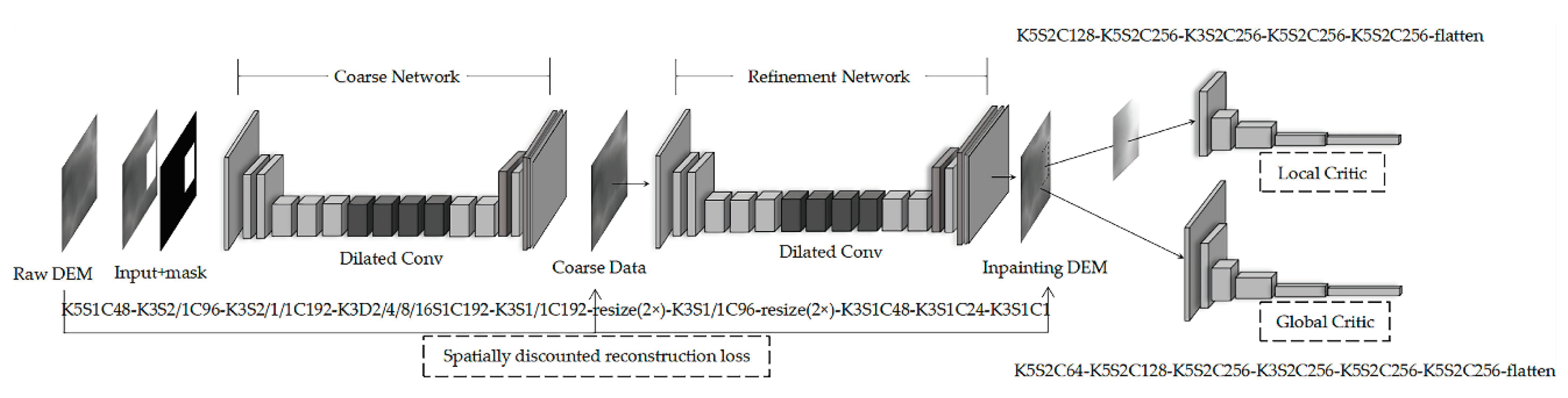
The network structure of the first part is shown in Figure 1, where K represents the kernel size, D represents the dilation, S represents the stride size, and C represents the channel number.
A DEM of the same size was adopted as the input of the network, while a missing area was randomly sampled at the front end of its training to ensure that the model post-training had the perceptual ability to complete void filling tasks with different numbers, sizes and areas.
DEM void filling based on the generated model has a network structure system of two stages. In the previous stage, the coarse network used reconstruction loss to assist the training and generate the approximate elevation value of the missing part. In the second stage, the detailed filling results are generated through the auxiliary continuous training of reconstruction loss and two GAN losses. The core significance of refinement network lies in the re-prediction of rough generated values so it has the ability to see a more complete field of vision than the missing area while having better feature representation than the coarse network.
2.1.2. Deep Generation Model Discriminant Loss
A WGAN uses earth mover’s (EM) distance to replace the Kullback–Leibler (KL) divergence in the GAN. The literature [24] described the WGAN as in Equation (1):
where all functions that satisfy the 1-Lioschitzlimit are represented by a neural network with a parameter and obtain the upper bound of . The reverse of this can be used to construct the discriminant loss function in Equation (2):
where in the formula.
The literature [20] proposed an improved version of the WGAN with a gradient penalty (WGAN-GP) term to eliminate the effect of gradient instability. A penalty term (= 1) was added on the basis of the above loss. Finally, a new discriminant loss function can be obtained to form Equation (3):
For the purpose of this study, the gradient penalty term is only used inside the hole, and the mask placed in Equation (4) is as follows:
The filling network that relied on global and local GAN losses for adversarial supervision training allowed for the learning of image features through inlining. Therefore, the network used the discriminant loss based on WGAN-GP to attach the output of the refinement network.
2.1.3. Spatially Discounted Reconstruction Loss
DEM void repair involves the prediction of different elevation values. For any given context information, there are different and semantic filling methods. A feasible repair result may be quite different from the original DEM. Under this condition, if the original data is used as the reference standard for calculating the reconstruction loss, it will cause a deviation in the model training process. The proposal of spatial attenuation reconstruction loss was reasonably applied to solve such problems. Since the semantic information of the hole boundary is far more than the information in the middle of the hole, if the mask with weight is used, the weight of each point to be inserted in the mask is , where is the distance from the point to be interpolated to the known sampling point. If the value of is set to less than 1, then as the point to be interpolated is closer to the center of the hole, the weight will decrease as the distance increases. The smaller center weight reduces the error effect that may be caused by the gap between the repair result and the original image.
2.2. Contextual Attention Layer
The contextual attention layer borrows (or copies) feature information from a known background to fill the relevant properties of the void area. In the network training process, the context focuses on the model matching the missing value (foreground) and the surrounding environment (background) features, using the normalized inner product to measure the matching between the foreground block and the background block as in Equation (5):
where represents the similarity of feature matching between the foreground and the background . One can calculate the weight () of each background block, select the optimal block and deconvolute it to get the foreground region.
Attention was paid to the existence of propagation to maintain the overall consistency of the image. The idea was based on the foreground block corresponding to the background block, and they may change together, such as in the similarity between the point to be interpolated and the value of the surrounding point. Taking left–right propagation as an example, a similarity degree similar to Equation (6) can be obtained:
where is the kernel size.
2.3. Unified Inpainting Network
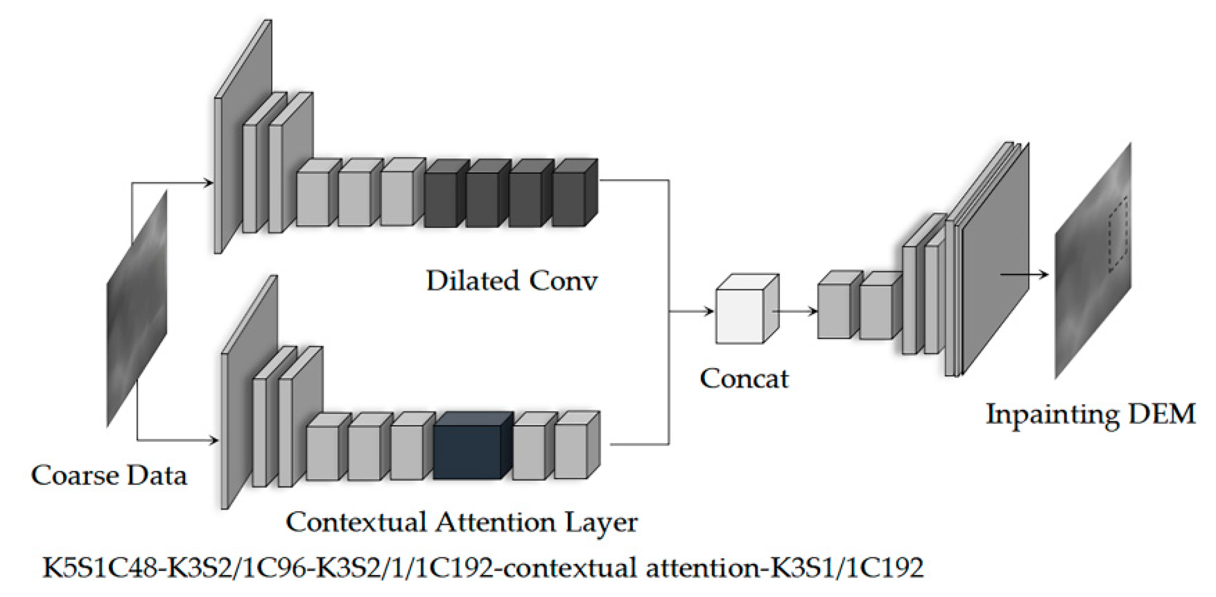
The network combined the context attention layer into the fine network and formed a parallel encoder, as shown in the second part of Figure 2.
The downlink encoder was trained to predict the output missing graph block, and the uplink encoder convolved out the foreground area. The output features of the two encoders were aggregated into a decoder, and the final deconvolution results were obtained.
In the filling task, is defined as the original DEM data. By randomly generating a mask , the input DEM is . The filling network takes and as inputs, and the DEM based on this output is . Then, one can find the filling result in the same position as the mask area in , map it to and get the final repaired DEM . The training process is as follows:
| Algorithm: DEM Null Filling |
| Input: with holes, mask . |
| Output: Final prediction . |
| 1: while has not reached convergence do |
| 2: Sample batch DEMs from training data. |
| 3: Generate masks with random holes for each . |
| 4: Create input data . |
| 5: The network allows and to be entered together. |
| 6: Get predicted DEMs data . |
| 7: Match the repaired area in to . |
| 8: Get the final forecast DEMs . |
| 9: Update the completion network with spatial discounted reconstruction loss and two WGAN-GP losses. |
| 10: end while |
2.4. Boundary Reprocessing
Bilateral filtering was selected in this paper to alias the DEM results, as the mapping behavior after filling brought certain boundary effects. The basic idea underlying bilateral filtering is to do it in the range of an image that traditional filters do in its domain. Two pixels can be close to one another—that is, occupy nearby spatial location—or they can be similar to one another; that is, they can have nearby values, possibly in a perceptually meaningful fashion [25]. The formula is defined as follows:
The above formula represents the product of the weight, calculated by the spatial proximity between each point and its central point , within a certain range of and the weight calculated by pixel value similarity. Through the convolution calculation, the DEM data were output. Finally, the obtained data were mapped to the repaired DEM data to eliminate the boundary effect.
3. Results
3.1. The Test Data
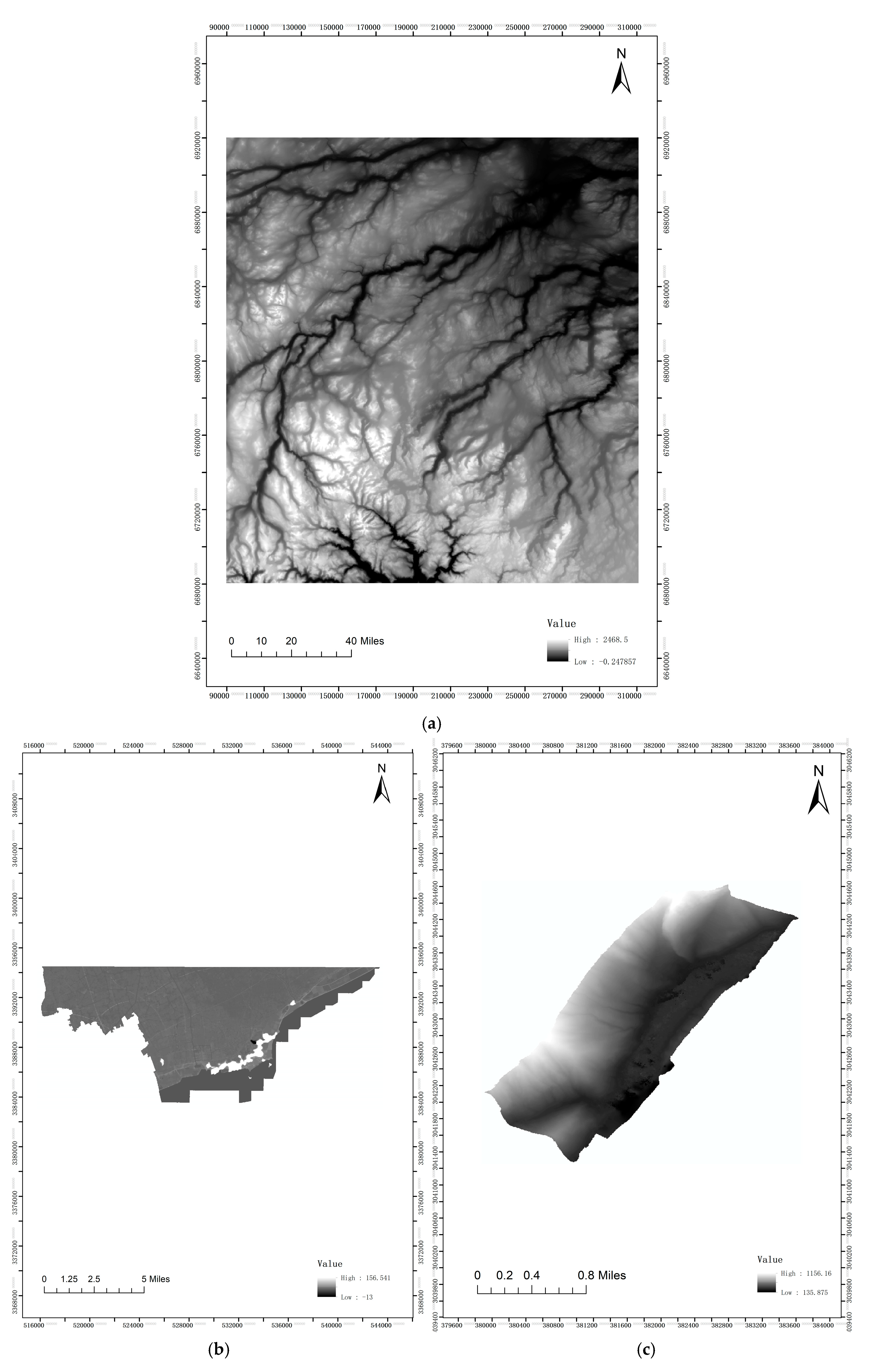
In order to illustrate the effectiveness and universality of this method, this paper selected the national elevation model of a region in Norway like Figure 3a as the data set to verify the prediction ability of the network. At the same time, the DEM data generated, based on actual photogrammetry projects in a place in Jiangsu province (gentle terrain) like Figure 3b and a place in Sichuan province (complex terrain) like Figure 3c, proved the generalization ability of the model. The data format of the national elevation model in Norway was USGS (U.S. Geological Survey) DEM. USGS DEM mainly has two types of grid forms; one is a Mercator projection (UTM) grid, and the other is a geographical coordinate grid divided into seconds. There were three reasons for choosing the national elevation model of a certain region in Norway as the data set. First, it was publicly available, and as an academic research endeavor, it had the value of reuse. Second, its data range was customizable in that the method in this paper relied on deep learning construction. Sufficient sample resources guaranteed the stable training of the network. Third, Norway’s diversity of terrain made it very suitable for extension to other parts of the world [23]. The data format is shown in Table 1.
The Norwegian data were pre-cut to generate 13,500 slice samples of 256 × 256 pixels in size, and then nine-tenths of the DEM data were randomly selected from them as the training sample set; the remaining one-tenth of the DEM data were used as the test samples. The training samples of the input into the network were normalized to enable the network to converge faster while solving the problem of gradient dispersion in a certain degree of deep networks. Meanwhile, the actual engineering generated data were mainly used to evaluate the generalization ability of the models trained by Norwegian datasets for different regions and resolutions, but consistent types of samples.
The network was completed under the TensorFlow deep learning framework. Based on the parameter recommendations in [19], the learning rate was set to 0.001, the parameters were Beta 1 = 0.5 and Beta 2 = 0.999 of the adaptive matrix estimation (Adam) optimizer, the batch size was 12, the number of iterations in one epoch was 1000 and the iteration lasted for 40 epochs. The entire training process would take about 26 h on a single NVIDIA GeForce RTX 2080 SUPER.
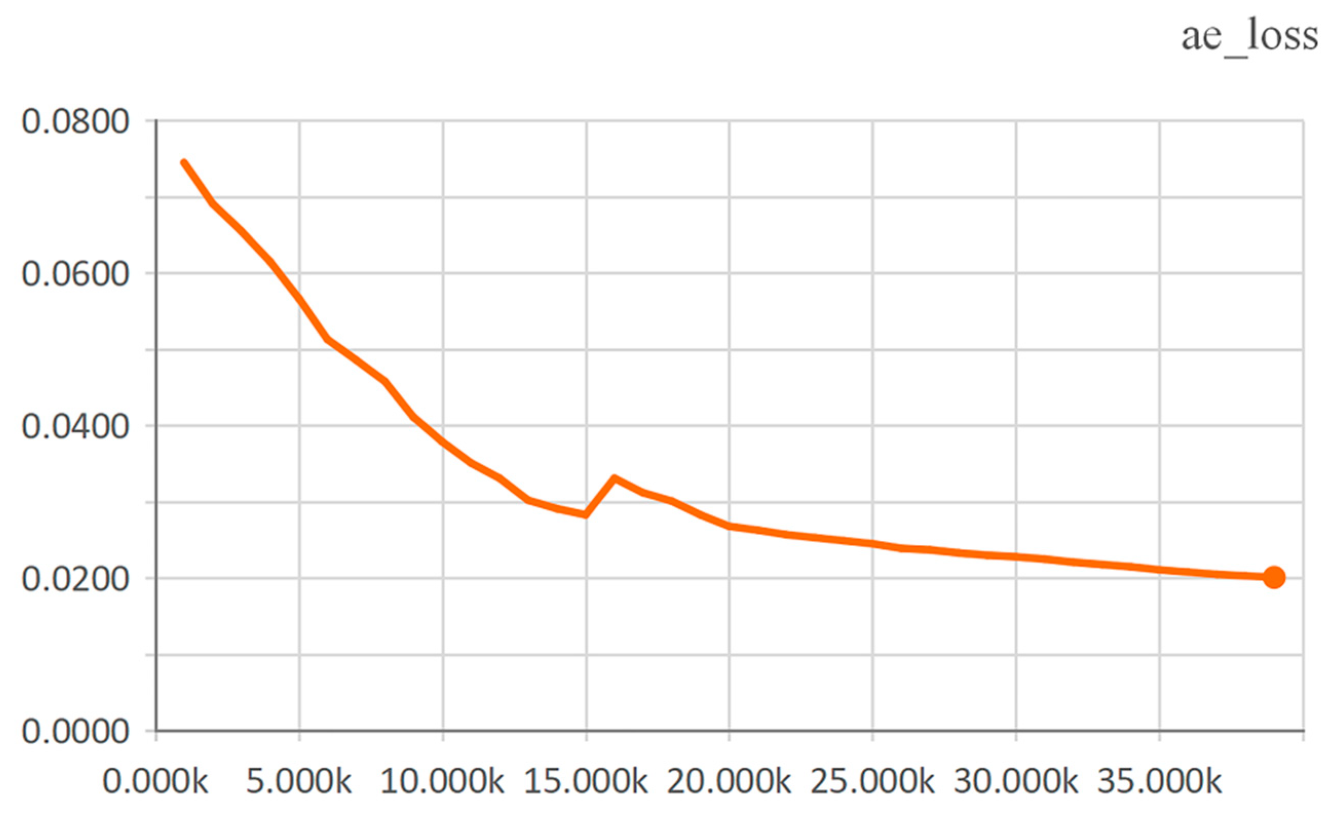
To simply illustrate the training process of the model, each generation output its corresponding spatially discounted reconstruction loss. As shown in Figure 4, the spatially discounted reconstruction loss was used to measure the reconstruction deviation between the predicted value and the true value during the training process. It was a reference standard for feasibility repair results, and its value reflected the quality of the model training.
Figure 4 reflects the stability of the training process. When iterating 16k times, the loss had abrupt changes. The reason was that the weights had been adjusted during the network iteration process, which led to jumps in the reconstruction loss. After the value, the gradient continued to be lower until it stabilized and converged.
3.2. The Evaluation Index
In order to quantitatively evaluate different repair methods and the repair method in this paper, the mean error (ME), root-mean-square error (RMSE) and predicted fit (R2) were adopted as the main indicators for detecting the accuracy of DEM void filling [26,27,28]. The calculation formulas were as follows:
where is the predicted elevation value of the point to be inserted, is the measured elevation value of the point to be inserted, is the total number of points to be inserted and is the measured average value of all the points to be inserted and participating in the calculation.
The RMSE was defined as the sum of the squares of the deviation between the observed value and the true value and the square root of the ratio of n to the number of observations to measure the deviation between the observed value and the true value. The smaller the RMSE value was, the closer the predicted elevation value was to the measured elevation value, and therefore the better the filling effect was. The closer the value of R2 was to 1, the higher the interpolation accuracy.
3.3. Experimental Results and Analysis
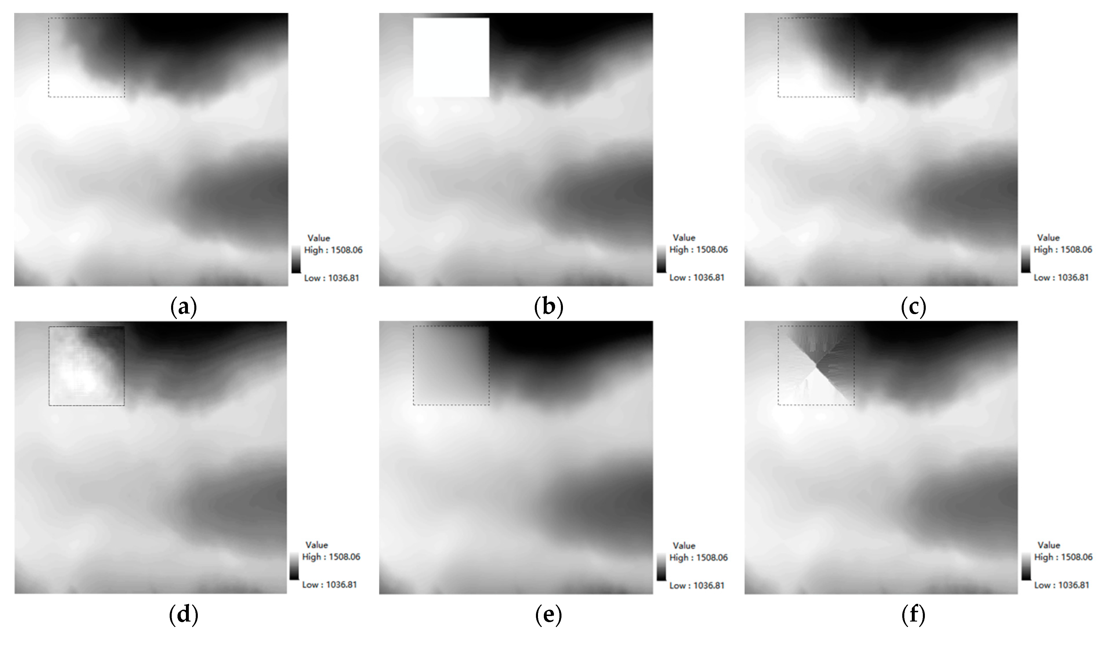
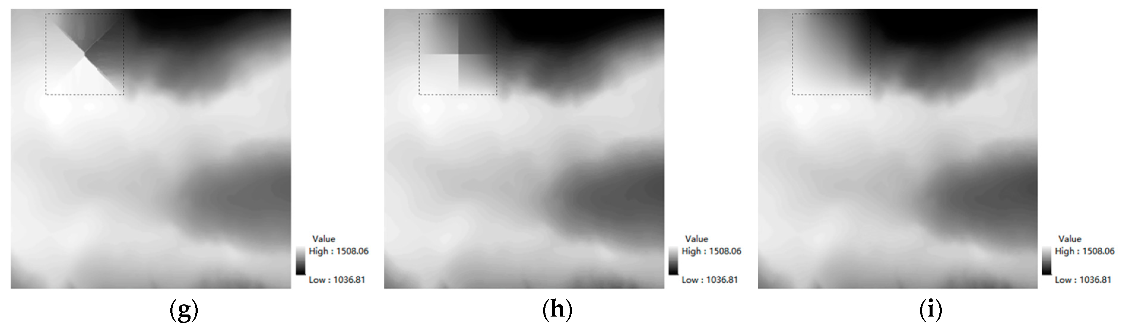
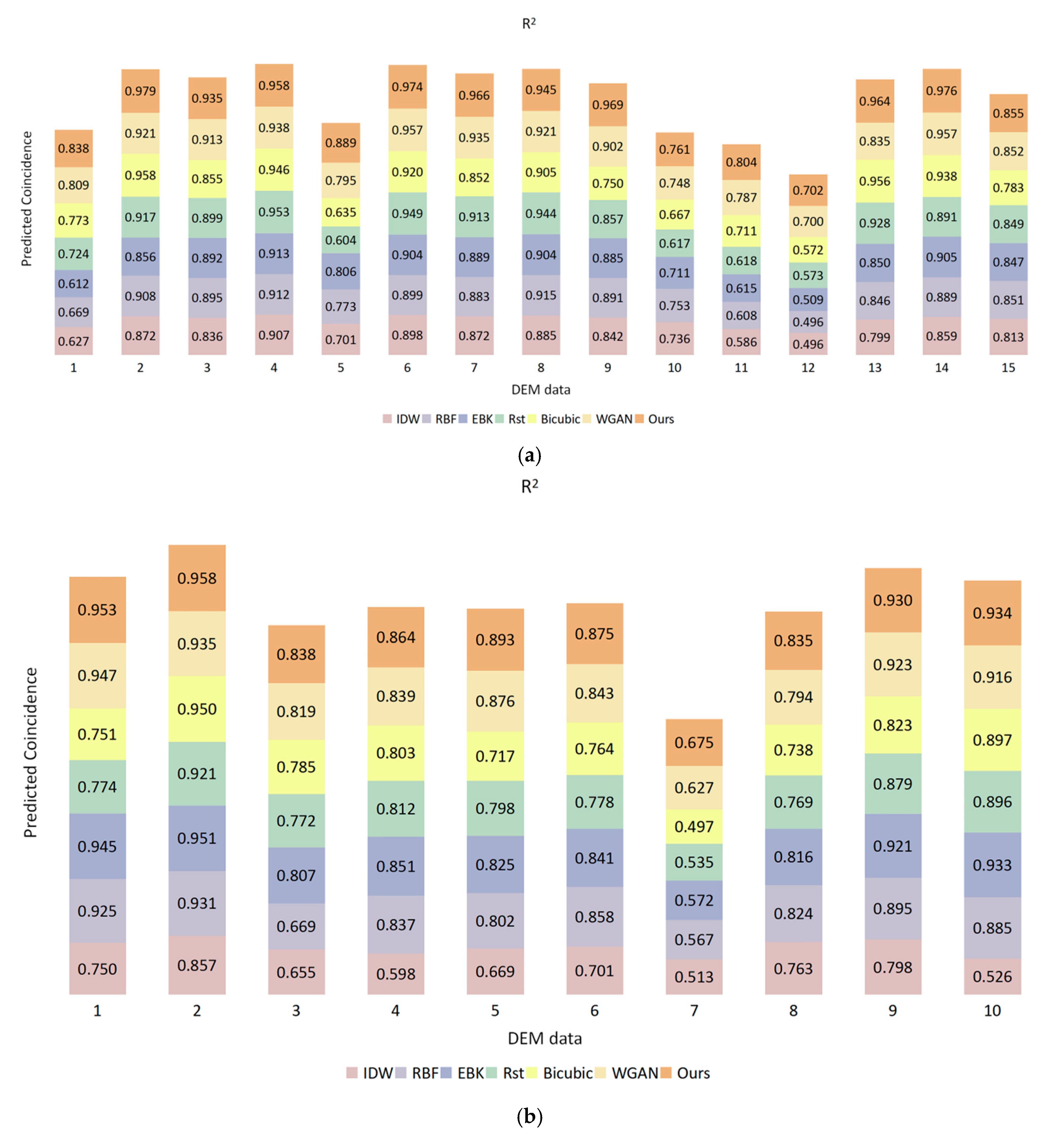
Based on the cut out DEM test set, 15 DEM data with gentle terrain and 10 DEM data with complex terrain were randomly selected for test verification. The extracted data are shown in Figure 5a and Figure 6a. The DEM data to be filled are shown in Figure 5b and Figure 6b. The given maximum size of the mask hole was 111 × 108, the number of data points to be filled was 11,988 pixels, the minimum size of the mask hole was 72 × 66 and the number of data points to be filled was 4752 pixels. For the DEM data with voids, the inverse distance weight (IDW) method, radial basis function (RBF) method, empirical Bayesian kriging (EBK) method, regular spline interpolation with tension (Rst), bicubic spline interpolation (Bicubic), Wasserstein GAN (WGAN) and the method in this paper were used to predict their missing elevation values.
It can be seen from the filling effect of the two-dimensional images in Figure 5 and Figure 6 that when filling DEM voids in different terrains, the method in this paper had strong characteristic expressiveness and an anti-interference ability. By comparing and analyzing the feature information of other methods, we could intuitively reflect that the DEM data generated by a WGAN were relatively scattered. Although the characteristics were obvious, they were not quite consistent with the original data. The IDW, Rst and Bicubic interpolation methods were fuzzy and overly smooth. The RBF and EBK interpolation methods had an obvious split phenomenon, and the data generated were relatively fragmented, which could not express the terrain features perfectly.
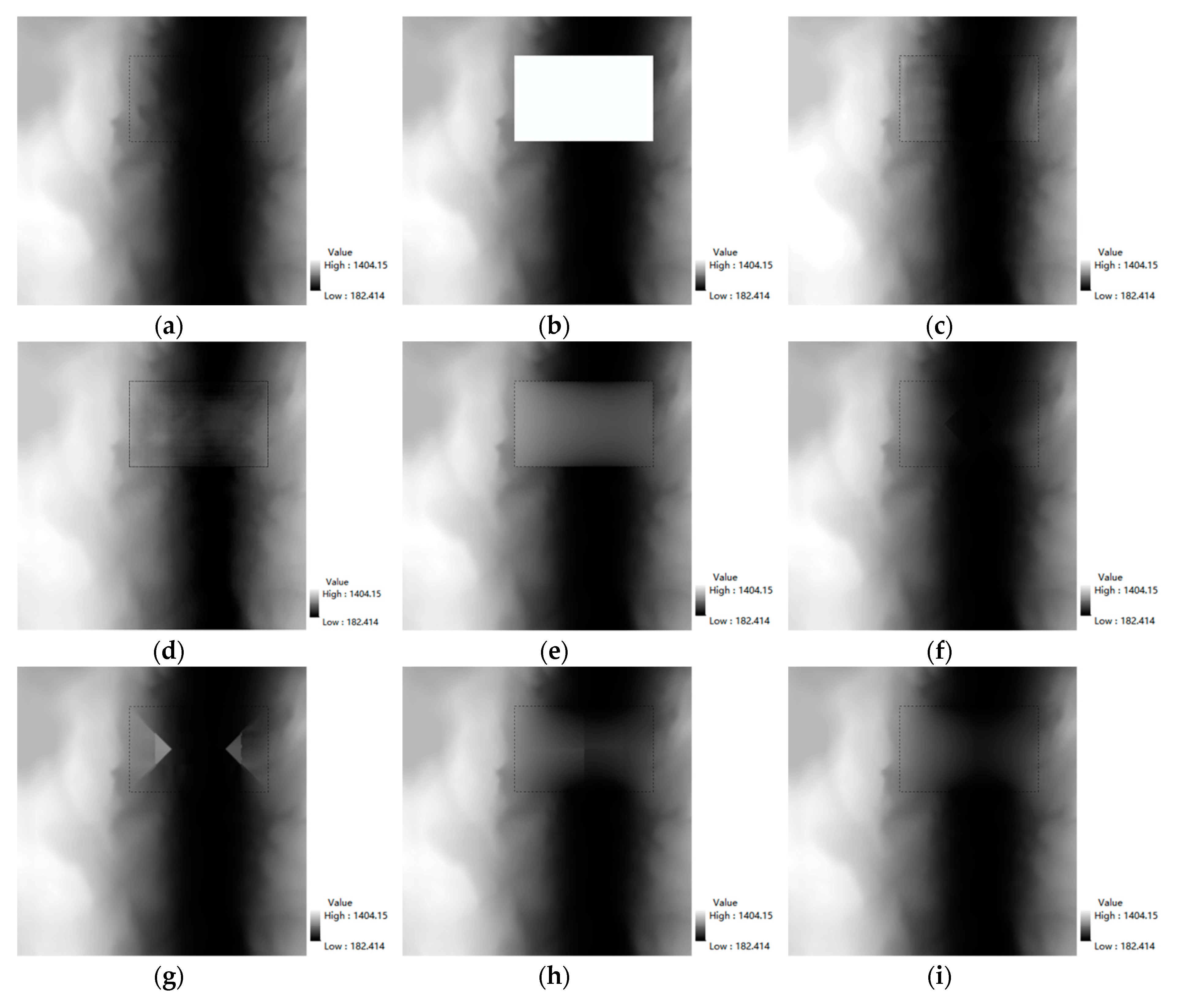
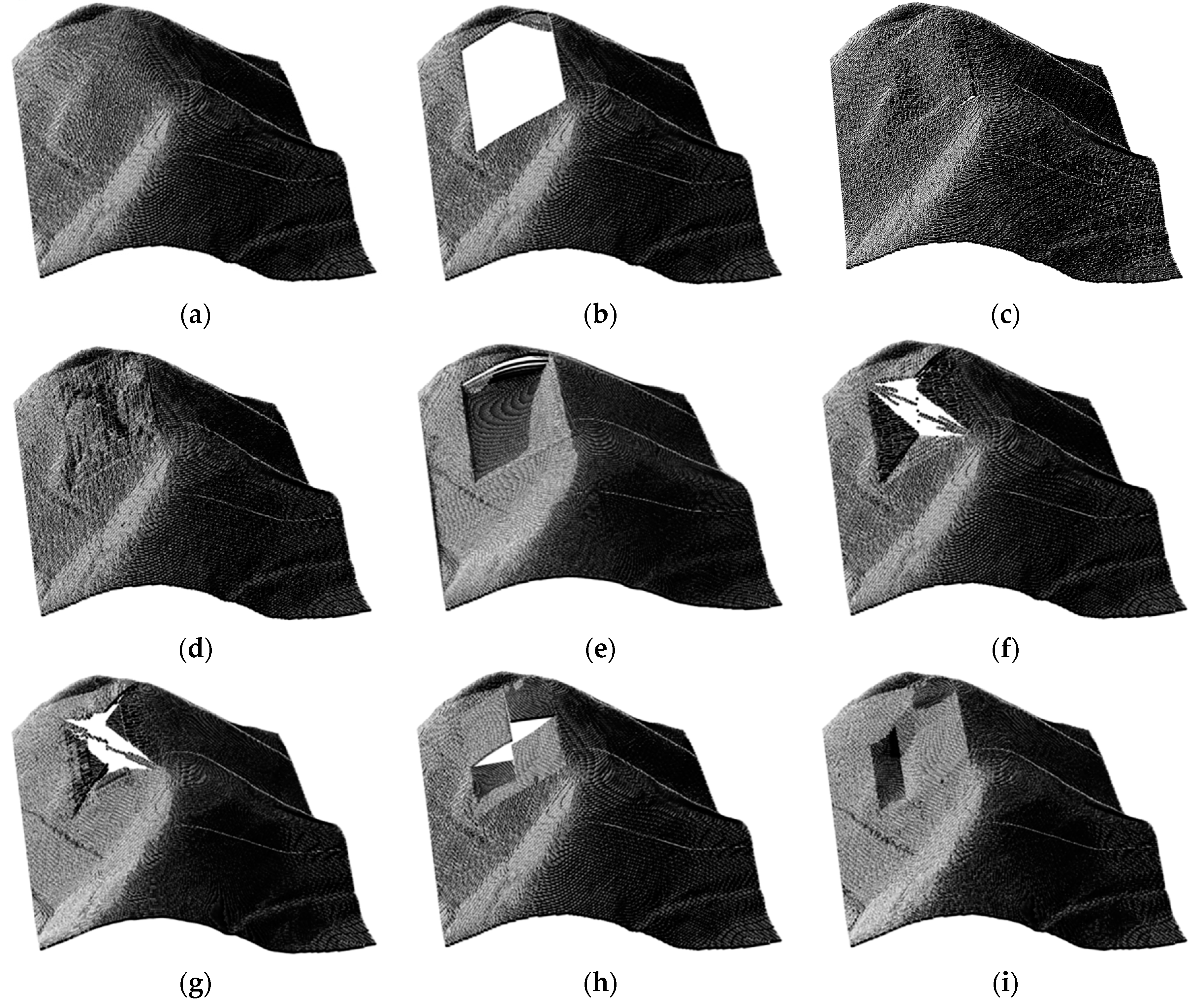
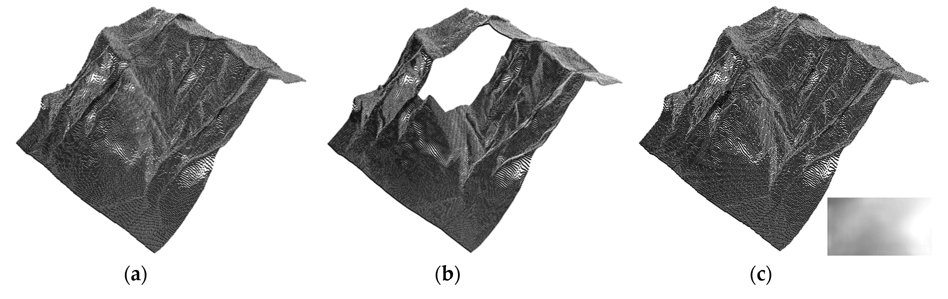
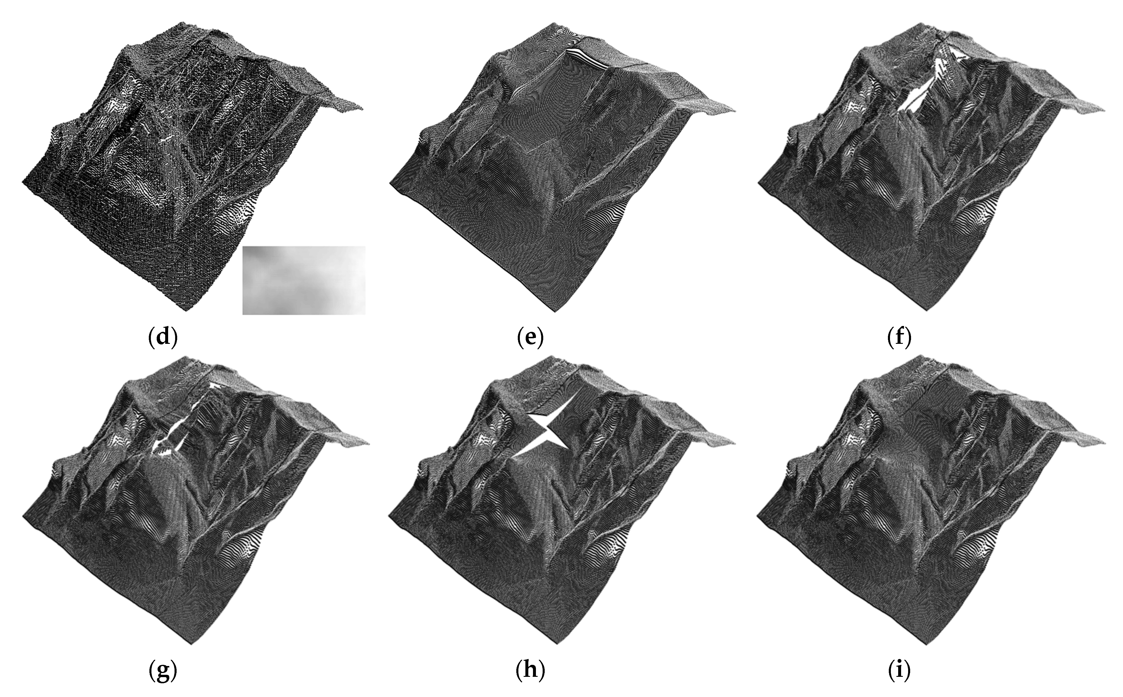
At the same time, in order to verify the strong generalization ability and the better expression ability of different terrains, the generation model was used to fill the holes in the DEM data of Jiangsu province and Sichuan province. The results of the 3D terrain test are shown in Figure 7 and Figure 8.
According to the analysis of the three-dimensional models in Figure 7 and Figure 8, the method in this paper had the same applicability to different terrains and data sources and could better conform to its spatial distribution. It would not be affected by different points, different weights or different models. Compared with the other methods, the restored elevation data was more stable, the accuracy was less disturbed, the three-dimensional terrain performed well and the generated semantic information was more reliable.
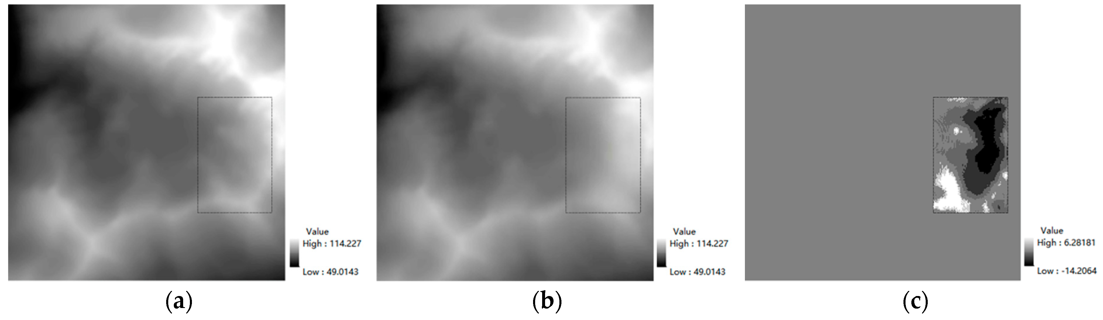
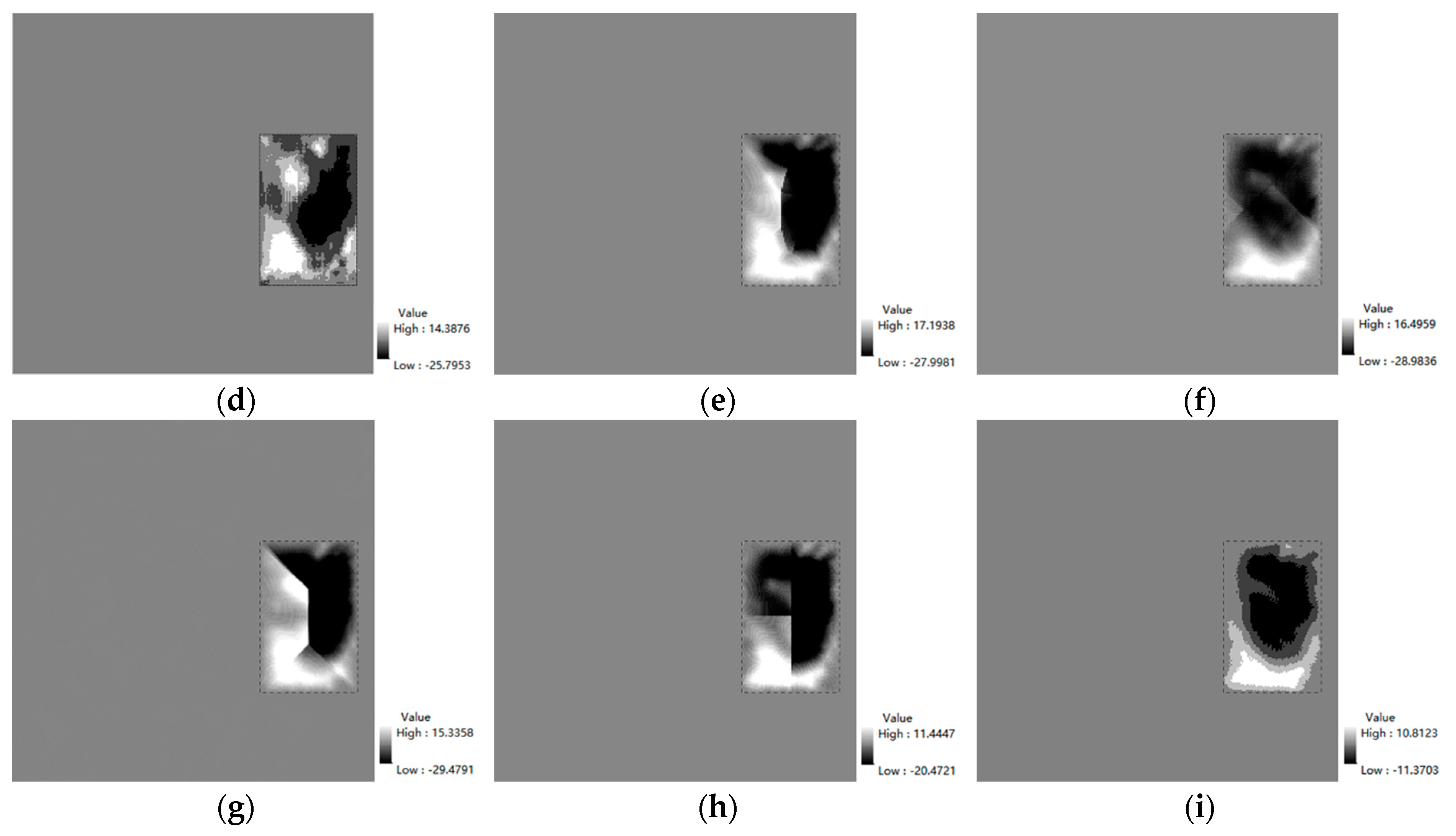
Next, we extracted the elevation value of the original DEM data in the mask range and the repair value in the corresponding range after filling and divided the gray level through the difference calculation. The gray scale difference based on the filled area was regarded as the foreground, and the gray scale difference of the unfilled area was regarded as the background, which could intuitively show the strength of the repair effect. The gray levels shown in Figure 9 are divided.
Comparing the foreground and background, the more the foreground gray tended to the background gray value, the smaller the gap between the two and the better the repair effect would be.
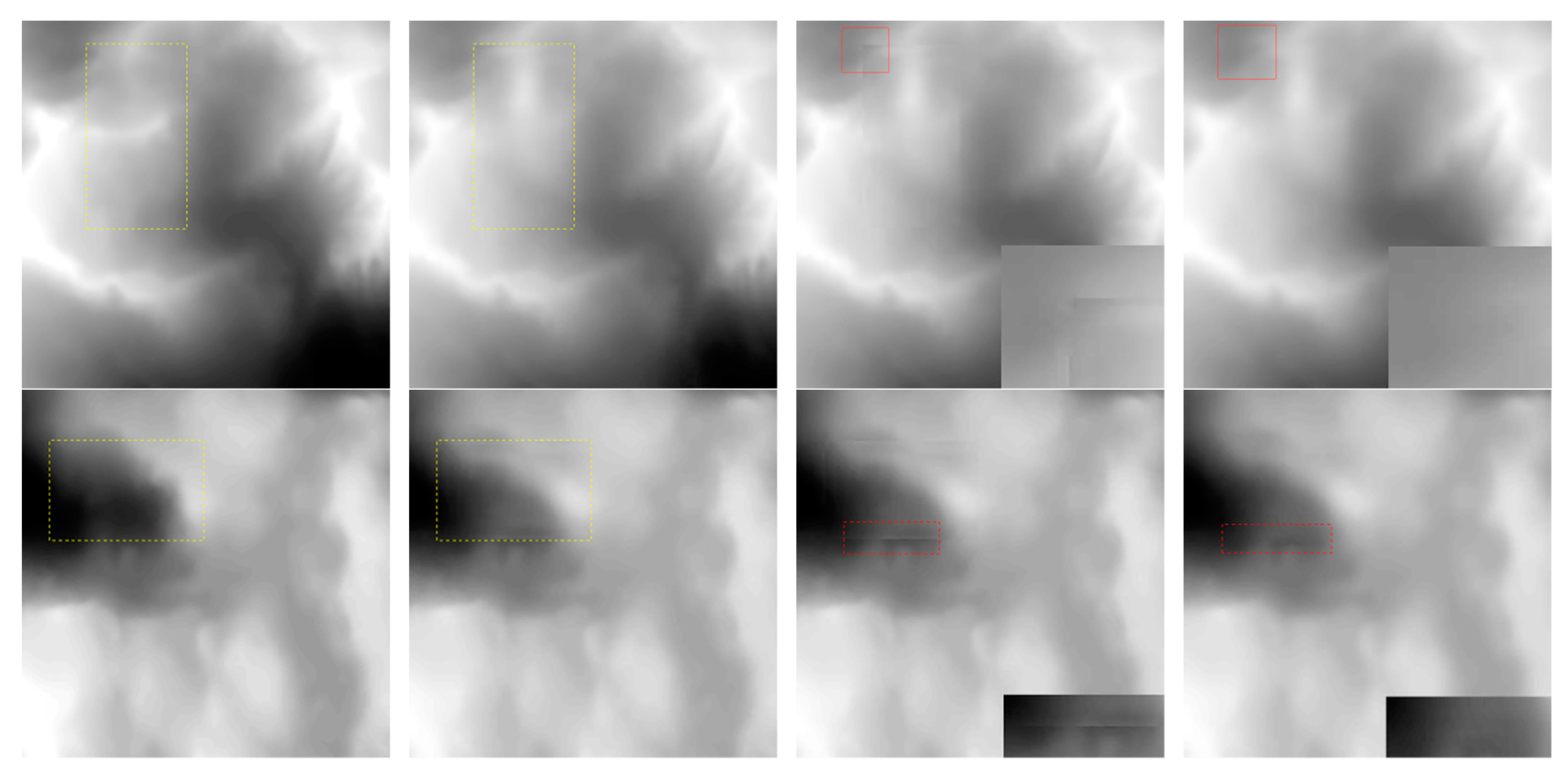
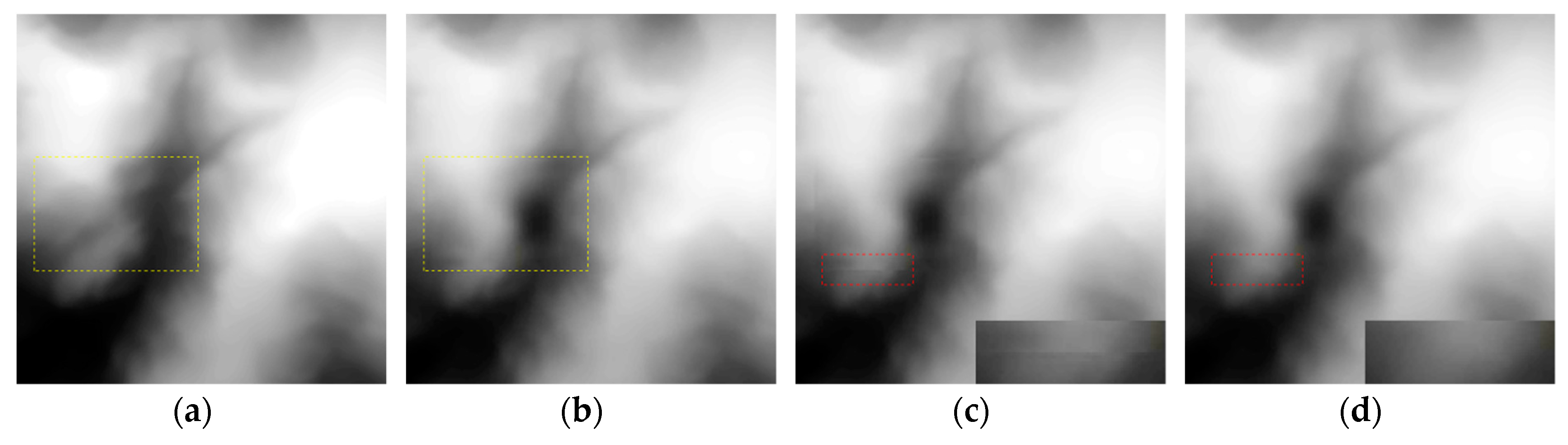
DEM filling with the help of deep learning pays more attention to the good visual repair of its texture and predicts a digital elevation model that has a higher degree of agreement with the original DEM. In DEM filling based on the contextual attention model, its network architecture focuses on the entire image’s features and uses the full image’s information to predict the elevation value of the missing part. Due to the mapping behavior after filling, the repaired DEM data had a marginal effect around the hole boundary and would have a certain visual sensory impact. The marginal effect is shown in Figure 10c.
In this paper, a local bilateral filtering algorithm was adopted to post-process the restored DEM results so as to eliminate the leaping errors generated at the boundary. The eliminated results are shown in Figure 10d.
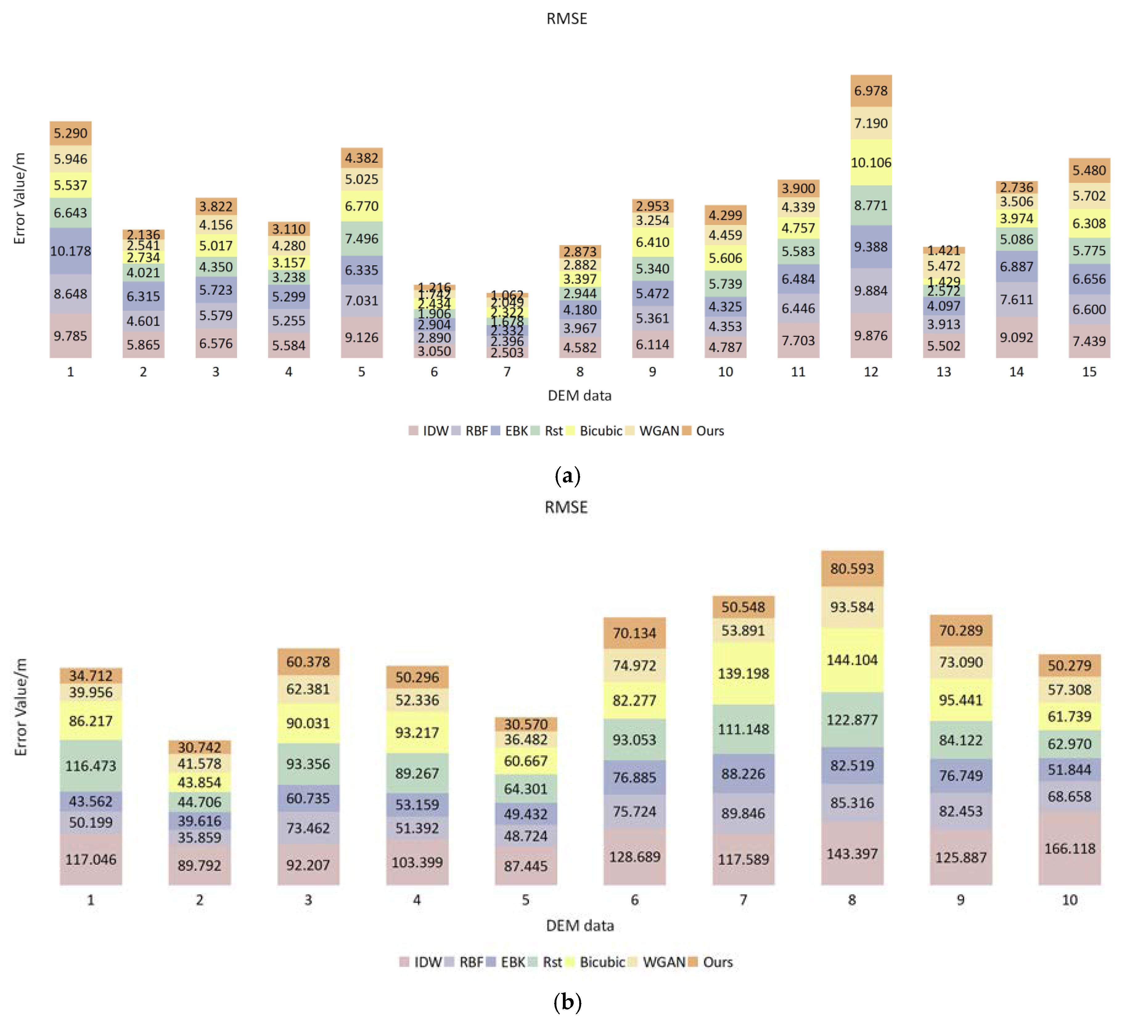
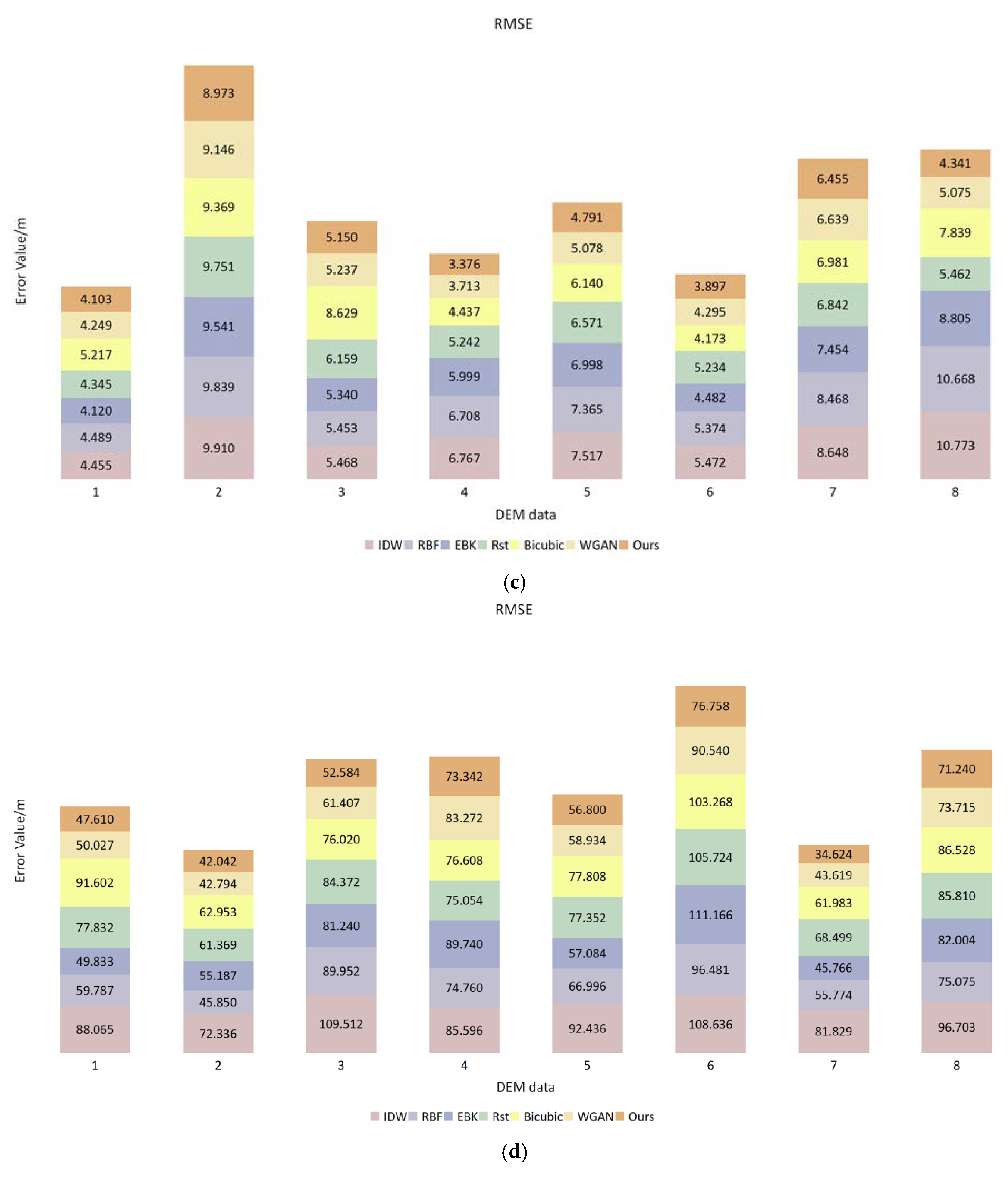
In order to make a fair comparison with the traditional method, this paper used the DEM filling results that had not been post-processed for comparative analysis. Figure 11 and Figure 12 show the objective comparative analysis of 15 groups of gentle test data, 10 groups of complex test data, 8 groups of Jiangsu province verification data and 8 groups of Sichuan province verification data after DEM filling by different methods and the method in this paper.
From the above error statistics and coincidence analysis, it can be seen that the proposed method had good, stable filling ability compared with the other methods. From both the feature information and the spatial structure, the model could predict its related characteristics well. At the same time, the data also showed that the model had the generalization ability to fill the DEMs of different data sources. The accuracy evaluation of different filling methods is shown in Table 2.
4. Discussion
We mainly put forward the application of this kind of model in surveying and mapping science and technology in order to discuss the popularization and application of a generating model in surveying and mapping. In the theory of probability and statistics, the generation model refers to the model which can generate the observation data randomly under the conditions of some implicit parameters. It assigns a joint probability distribution to the observation value and the labeled data sequence. In machine learning, a generative model can be used to model data directly or to establish conditional probability distribution among variables.
The introduction of a discriminate model leads to the emergence of a game type training process. The use of this kind of neural network as the model type is called a generative confrontation network (GAN). A GAN and its improvement [24,29,30,31,32] make generative models become a hot research direction of artificial intelligence technology. At present, it has been applied in Natural Language Processing (NLP), image generation, super-resolution, image restoration and other fields.
Extended to the current research of surveying and mapping disciplines, we have always believed that such models can be better applied in the following aspects:
- In the construction and repair of 3D models, the data collected by 3D sensors are often affected by occlusion, sensor noise and light, resulting in the incompleteness of 3D models and the generation of noise. However, one can understand and describe the geometry of the entire building based on a damaged 3D model. The method described in [33] attempted to imitate this ability and reconstruct a complete three-dimensional model from incomplete data.
- Cloud removal. Satellite images are increasingly used in a variety of applications, including monitoring the environment, mapping economic development, crop type classification, land cover and measuring the leaf index. However, satellite images are often obscured by clouds, which cover about two-thirds of the world. Thick clouds hide the content of the image, and even thin, translucent clouds can greatly affect the effectiveness of satellite images by distorting the ground below. Therefore, it is the first important step in most satellite image analysis to remove cloud cover and generate cloud free images [34].
- Target identification. In recent years, deep learning has achieved great success in the field of image object recognition. Its advantage is that it can use a large amount of data to train the network, learn the characteristics of the goal, avoid complex preprocessing and achieve better results. Presented in [35] was a semi-supervised learning method based on standard deep convolution generative adversarial networks (DCGAN) for the target recognition of synthetic aperture radar images.
5. Conclusions
With regard to the remaining problems in the traditional method of DEM void filling, this paper introduced a method based on the algorithm of deep learning, aiming to repair the DEM. At the first stage of the network, the global and local countermeasures were used to ensure the consistency of the predicted data. At its second stage, the contextual attention layer was combined to perceive global information and enhance the representational ability of the data texture structure. In order to verify the effectiveness and universality of this proposed method, three kinds of data were compared with different repair methods. As indicated by the results, the traditional method focused more on the image’s gray value and could not interpolate the missing data of elevation well, leading to the obtained DEM being broken and discontinuous. Meanwhile, the repairing results obtained by the WGAN manifested weakness in its characteristic expressiveness, which may have failed in soundly obtaining the prediction results. By the method of DEM void filling, as illustrated in this paper, it is easier to grasp the elevation information and its related characteristics so that the post-repair data would possess a certain degree of space continuity and heterogeneity. In this way, the post-repair data would possess higher alignment with the original DEM data and manifest excellence in the forecast for filling from different data sources, so as to be a kind of filling method with high reliability and strong adaptability.
Author Contributions
Chunsen Zhang and Shu Shi gave the conceptualization and methodology of the manuscript. The software implementation of the method was given by Shu Shi and Yingwei Ge. Hengheng Liu completed the data validation. Weihong Cui’s role was project administration and supervision. All authors have read and agreed to the published version of the manuscript.
Funding
This work was supported in part by the Open Research Fund of the State Key Laboratory of Information Engineering in Surveying, Mapping and Remote Sensing, Wuhan University, under Project 18R01, in part by the China Postdoctoral Science Foundation under Project 2018M642915, and in part by the Grant of Shaanxi Provincial Department of Education under Project 19JK0522.
Conflicts of Interest
The authors declare no conflict of interest.
References
- Nizar, P.; Murat, U. An Experimental Analysis of Digital Elevation Models Generated with Lidar Data and UAV Photogrammetry. J. Indian Soc. Remote Sens. 2018, 46, 1135–1142. [Google Scholar]
- Zhu, Q.; Tian, Y.X.; Zhang, Y.T. Method of Automatic Extraction of Catchment Area and Its Subarea from DEM of Regular Grid. Acta Geod. Cartogr. Sin. 2005, 34, 129–133. [Google Scholar]
- Yue, Z.S.; Zhang, Y.J.; Duan, Y.S.; Yu, L. DEM Assisted Shadow Detection and Topography Correction of Satellite Remote Sensing Images in Mountainous Area. Acta Geod. Cartogr. Sin. 2018, 47, 113–122. [Google Scholar]
- Krauß, T.; D’Angelo, P. Morphological Filling of Digital Elevation Models. In Proceedings of the International Archives of the Photogrammetry, Remote Sensing and Spatial Information Sciences, Volume XXXVIII-4/W19, 2011ISPRS Hannover 2011 Workshop, Hannover, Germany, 14–17 June 2011. [Google Scholar]
- Li, S.J.; Dai, W.; Xiong, L.Y.; Tang, G.A. Uncertainty of the morphological feature expression of loess erosional gully affected by DEM resolution. J. Geo-Inf. Sci. 2020, 22, 338–350. [Google Scholar]
- Zhang, X.; Zhou, J.M.; Liu, Z.P. DEM extraction and precision evaluation of mountain glaciers in the Qianghai-Tibet Plateau based on KH-9 data: Take the Purog Kangri Glacier and the Jiong Glacier as example. J. Glaciol. Geocryol. 2019, 41, 27–35. [Google Scholar]
- Lv, X.K.; Wang, Q.S.; Li, Y.F. Elimination method of TIN massive terrain crack based on terrain feature. Comput. Eng. 2019, 45, 232–236. [Google Scholar]
- Yue, Y.L.; Luo, M.L.; Zhang, B. Study on Spatial Distribution of DEM Interpolation Errors in the Gully of Dry-Hot Valley. Geomat. Inf. Sci. Wuhan Univ. 2018, 43, 1122–1128. [Google Scholar]
- Hou, X.X.; Huang, G.M.; Zhao, Z.; Li, W.T. A void hole filling method for airborne InSAR DEM based on FBM. Sci. Surv. Mapp. 2017, 42, 141–147. [Google Scholar]
- Zhang, J.Q.; Li, C.L.; Guo, B.Y. A Fast Surface Reconstruction Algorithm for Unorganized Points Based on Tangent Plane Projection. Geomat. Inf. Sci. Wuhan Univ. 2011, 36, 757–762. [Google Scholar]
- Nielson, G.M.; Hagen, H.; Lee, K. Implicit fitting of point cloud data using radial hermite basis functions. Computing 2007, 79, 301–307. [Google Scholar] [CrossRef]
- Du, X.W.; Yang, X.Y.; Liang, X.Z. Surface Reconstruction of 3D Scattered Data with Radial Basis Functions. Commun. Math. Res. 2010, 2, 89–98. [Google Scholar]
- Ye, J.F.; Gao, Z.S.; Liu, X.L.; Wang, W.; Zhang, C.Y. Freeform Surface Reconstruction Based on Zernike Polynomials and Radial Basis Function. Acta Opt. Sin. 2014, 34, 233–241. [Google Scholar]
- Liu, S.J.; Xiao, J.T.; Hu, L.; Liu, X.R. Implicit surfaces from polygon soup with compactly supported radial basis functions. Vis. Comput. 2018, 34, 779–791. [Google Scholar] [CrossRef]
- Lv, H.Y.; Sheng, Y.H.; Li, J.; Duan, P.; Zhang, S.Y. An Adaptive Parallel CSRBF Terrain Interpolation Method Based on RASM. Geomat. Inf. Sci. Wuhan Univ. 2017, 42, 1316–1322. [Google Scholar]
- Liu, X.Y.; Wang, H.; Chen, C.S.; Wang, Q. Implicit surface reconstruction with radial basis functions via PDEs. Eng. Anal. Bound. Elem. 2020, 110, 95–103. [Google Scholar] [CrossRef]
- Iizuka, S.; Simo-Serra, E.; Ishikawa, H. Globally and locally consistent image completion. ACM Trans. Graph. 2017, 36, 1–14. [Google Scholar] [CrossRef]
- Pathak, D.; Krahenbuhl, P.; Donahue, J.; Darrell, T. Context Encoders: Feature Learning by Inpainting. arXiv 2016, arXiv:1604.07379. [Google Scholar]
- Yu, J.H.; Lin, Z.; Yang, J.M.; Shen, X.H. Generative Image Inpainting with Contextual Attention. arXiv 2018, arXiv:1801.07892. [Google Scholar]
- Gulrajani, I.; Ahmed, F.; Arjovsky, M.; Dumoulin, V.; Courvile, A. Improved Training of Wasserstein GANs. arXiv 2017, arXiv:1704.00028. [Google Scholar]
- Zhu, D.; Cheng, X.M.; Zhang, F.; Yao, X.; Gao, Y.; Liu, Y. Spatial interpolation using conditional generative adversarial neural networks. Int. J. Geogr. Inf. Sci. 2020, 34, 735–758. [Google Scholar] [CrossRef]
- Dong, G.S.; Chen, F.; Ren, P. Filling SRTM Void Data via Conditional Adversarial Networks. In Proceedings of the IGARSS 2018—2018 IEEE International Geoscience and Remote Sensing Symposium, Valencia, Spain, 22–27 July 2018. [Google Scholar]
- Gavriil, K.; Muntingh, G.; Barrowclough, O.J.D. Void Filling of Digital Elevation Models with Deep Generative Models. arXiv 2018, arXiv:1811.12693. [Google Scholar] [CrossRef]
- Arjovsky, M.; Chintala, S.; Bottou, L. Wasserstein GAN. arXiv 2017, arXiv:1701.07875. [Google Scholar]
- Amante, C.J.; Eakins, B.W. Accuracy of Interpolated Bathymetry in Digital Elevation Models. J. Coast. Res. 2016, 76, 123–133. [Google Scholar] [CrossRef] [Green Version]
- Chen, C.F.; Yue, T.X.; Du, Z.P.; Lu, Y.M. DEM construction based on HASM and related error analysis. J. Remote Sens. 2010, 14, 80–89. [Google Scholar]
- Tang, G.A.; Gong, J.Y.; Chen, Z.J.; Cheng, Y.H.; Wang, Z.H. A Simulation on the Accuracy of DEM Terrain Representation. Acta Geod. Cartogr. Sin. 2001, 30, 361–365. [Google Scholar]
- Tomasi, C.; Manduchi, R. Bilateral filtering for gray and color images. In Proceedings of the Sixth International Conference on Computer Vision (IEEE Cat. No.98CH36271), Bombay, India, 7 January 1998. [Google Scholar]
- Ian, G.; Jean, P.A.; Mehdi, M.; Bing, X.; David, W.F.; Sherjil, Q.; Aaron, C.; Yoshua, B. Generative Adversarial Nets. arXiv 2014, arXiv:1406.2661. [Google Scholar]
- Radford, A.; Metz, L.; Chintala, S. UnsupervisedRepresentation Learning with Deep Convolutional Generative Adversarial Networks. arXiv 2015, arXiv:1511.06434. [Google Scholar]
- Odena, A. Semi-Supervised Learning with Generative Adversarial Networks. arXiv 2016, arXiv:1606.01583. [Google Scholar]
- Karnewar, A.; Wang, O. MSG-GAN: Multi-Scale Gradients for Generative Adversarial Networks. arXiv 2019, arXiv:1903.06048. [Google Scholar]
- Wang, W.Y.; Huang, Q.G.; You, S.Y.; Yang, C.; Neumann, U. Shape Inpainting using 3D Generative Adversarial Network and Recurrent Convolutional Networks. arXiv 2017, arXiv:1711.06375. [Google Scholar]
- Sarukkai, V.; Jain, A.; Uzkent, B.; Ermon, S. Cloud Removal in Satellite Images Using Spatiotemporal Generative Networks. arXiv 2019, arXiv:1912.06838. [Google Scholar]
- Gao, F.; Yang, Y.; Wang, J.; Sun, J.P.; Yang, E.F.; Zhou, H.Y. A Deep Convolutional Generative Adversarial Networks (DCGANs)-Based Semi-Supervised Method for Object Recognition in Synthetic Aperture Radar (SAR) Images. Remote Sens. 2018, 10, 846. [Google Scholar] [CrossRef] [Green Version]
Figure 1.
Network structure schematic.

Figure 2.
Unified inpainting network.

Figure 3.
DEM data. (a) Data of Norway; (b) data of a place in Jiangsu province; and (c) data of a place in Sichuan province.
Figure 3.
DEM data. (a) Data of Norway; (b) data of a place in Jiangsu province; and (c) data of a place in Sichuan province.

Figure 4.
Spatially discounted reconstruction loss.

Figure 5.
Digital elevation model (DEM) filling results in Norway (gentle terrain). (a) Raw DEM data; (b) DEM data with a void; (c) our method; (d) Wasserstein generative adversarial network (WGAN) method; (e) inverse distance weight (IDW) method; (f) radial basis function (RBF) method; (g) empirical Bayesian kriging (EBK); (h) regular spline interpolation with tension (Rst); and (i) bicubic spline interpolation (Bicubic).


Figure 6.
DEM filling results in Norway (complex terrain). (a) Raw DEM data; (b) DEM data with a void; (c) our method; (d) WGAN method; (e) IDW method; (f) RBF method; (g) EBK; (h) Rst; and (i) Bicubic.
Figure 6.
DEM filling results in Norway (complex terrain). (a) Raw DEM data; (b) DEM data with a void; (c) our method; (d) WGAN method; (e) IDW method; (f) RBF method; (g) EBK; (h) Rst; and (i) Bicubic.

Figure 7.
DEM 3D terrain filling results of a certain place in Jiangsu province (gentle terrain). (a) Raw DEM data; (b) DEM data with a void; (c) our method; (d) WGAN method; (e) IDW method; (f) RBF method; (g) EBK; (h) Rst; and (i) Bicubic.
Figure 7.
DEM 3D terrain filling results of a certain place in Jiangsu province (gentle terrain). (a) Raw DEM data; (b) DEM data with a void; (c) our method; (d) WGAN method; (e) IDW method; (f) RBF method; (g) EBK; (h) Rst; and (i) Bicubic.

Figure 8.
DEM 3D terrain filling results of a certain place in Sichuan province (complex terrain). (a) Raw DEM data; (b) DEM data with a void; (c) our method (the image in the lower right corner is a direct comparison of the results generated by the two methods); (d) WGAN method; (e) IDW method; (f) RBF method; (g) EBK; (h) Rst; and (i) Bicubic.


Figure 9.
Subtraction calculation. (a) Raw DEM data; (b) our result; (c) raw DEM minus our result; (d) raw DEM minus the WGAN result; (e) raw DEM minus the IDW result; (f) raw DEM minus the RBF result; (g) raw DEM minus the EBK result; (h) raw DEM minus the Rst result; and (i) raw DEM minus the Bicubic result.


Figure 10.
Marginal effects of repair results. (a) The column is the original DEM data; (b) the column is the DEM data after filling; (c) the column is marginalization effect; and (d) the column is the elimination of marginalization. (The data before and after repair are shown in the yellow box, and the data before and after the marginalization effect are smoothed in the red box).


Figure 11.
The root-mean-square error. (a) Test data for Norway (gentle terrain); (b) test data for Norway (complex terrain); (c) verification data of a place in Jiangsu province; and (d) verification data of a place in Sichuan province.
Figure 11.
The root-mean-square error. (a) Test data for Norway (gentle terrain); (b) test data for Norway (complex terrain); (c) verification data of a place in Jiangsu province; and (d) verification data of a place in Sichuan province.


Figure 12.
Coincidence prediction. (a) Test data for Norway (gentle terrain); (b) test data for Norway (complex terrain); (c) verification data of a place in Jiangsu province; and (d) verification data of a place in Sichuan province.
Figure 12.
Coincidence prediction. (a) Test data for Norway (gentle terrain); (b) test data for Norway (complex terrain); (c) verification data of a place in Jiangsu province; and (d) verification data of a place in Sichuan province.


Table 1.
Data parameters.
| Data | Time | Resolution | Size | Maximum Height | Generation Type |
|---|---|---|---|---|---|
| Norway | × | 10 m | 30,041 × 30,041 | 2468 m | UAV Photogrammetry |
| Jiangsu | 2015 | 2 m | 14,307 × 5708 | 170 m | |
| Sichuan | 2018 | 5 m | 3896 × 4523 | 1020 m |
Table 2.
Accuracy evaluation of filling methods.
(a) Accuracy evaluation of Norway test data (gentle terrain).
| Method | IDW | RBF | EBK | Rst | Bicubic | WGAN | Ours | |
|---|---|---|---|---|---|---|---|---|
| Indicator | ||||||||
| RMSE/m | 6.506 | 5.636 | 5.772 | 4.743 | 4.664 | 4.169 | 3.444 | |
| R2 | 0.782 | 0.813 | 0.807 | 0.816 | 0.815 | 0.865 | 0.901 | |
(b) Accuracy evaluation of Norway test data (complex terrain).
| Method | IDW | RBF | EBK | Rst | Bicubic | WGAN | Ours | |
|---|---|---|---|---|---|---|---|---|
| Indicator | ||||||||
| RMSE/m | 117.157 | 66.163 | 62.273 | 88.227 | 89.675 | 58.559 | 52.854 | |
| R2 | 0.683 | 0.819 | 0.846 | 0.793 | 0.773 | 0.852 | 0.876 | |
(c) Accuracy evaluation of a place in Jiangsu province’s validation data.
| Method | IDW | RBF | EBK | Rst | Bicubic | WGAN | Ours | |
|---|---|---|---|---|---|---|---|---|
| Indicator | ||||||||
| RMSE/m | 7.376 | 7.296 | 6.706 | 6.201 | 6.598 | 5.429 | 5.136 | |
| R2 | 0.839 | 0.838 | 0.860 | 0.848 | 0.843 | 0.887 | 0.893 | |
(d) Accuracy evaluation of a place in Sichuan province’s validation data.
| Method | IDW | RBF | EBK | Rst | Bicubic | WGAN | Ours | |
|---|---|---|---|---|---|---|---|---|
| Indicator | ||||||||
| RMSE/m | 91.889 | 70.584 | 71.503 | 79.502 | 79.596 | 63.039 | 56.875 | |
| R2 | 0.713 | 0.774 | 0.778 | 0.792 | 0.779 | 0.827 | 0.852 | |
Publisher’s Note: MDPI stays neutral with regard to jurisdictional claims in published maps and institutional affiliations. |
© 2020 by the authors. Licensee MDPI, Basel, Switzerland. This article is an open access article distributed under the terms and conditions of the Creative Commons Attribution (CC BY) license (http://creativecommons.org/licenses/by/4.0/).
Share and Cite
MDPI and ACS Style
Zhang, C.; Shi, S.; Ge, Y.; Liu, H.; Cui, W. DEM Void Filling Based on Context Attention Generation Model. ISPRS Int. J. Geo-Inf. 2020, 9, 734. https://0-doi-org.brum.beds.ac.uk/10.3390/ijgi9120734
AMA Style
Zhang C, Shi S, Ge Y, Liu H, Cui W. DEM Void Filling Based on Context Attention Generation Model. ISPRS International Journal of Geo-Information. 2020; 9(12):734. https://0-doi-org.brum.beds.ac.uk/10.3390/ijgi9120734
Chicago/Turabian StyleZhang, Chunsen, Shu Shi, Yingwei Ge, Hengheng Liu, and Weihong Cui. 2020. "DEM Void Filling Based on Context Attention Generation Model" ISPRS International Journal of Geo-Information 9, no. 12: 734. https://0-doi-org.brum.beds.ac.uk/10.3390/ijgi9120734
Note that from the first issue of 2016, this journal uses article numbers instead of page numbers. See further details here.