Towards Automated Binding Affinity Prediction Using an Iterative Linear Interaction Energy Approach


Abstract
:
1. Introduction
2. Computational Methods
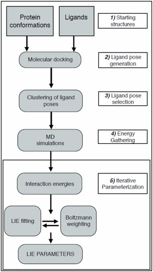
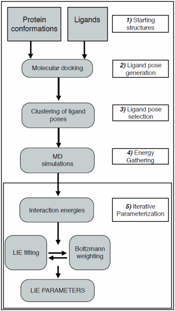
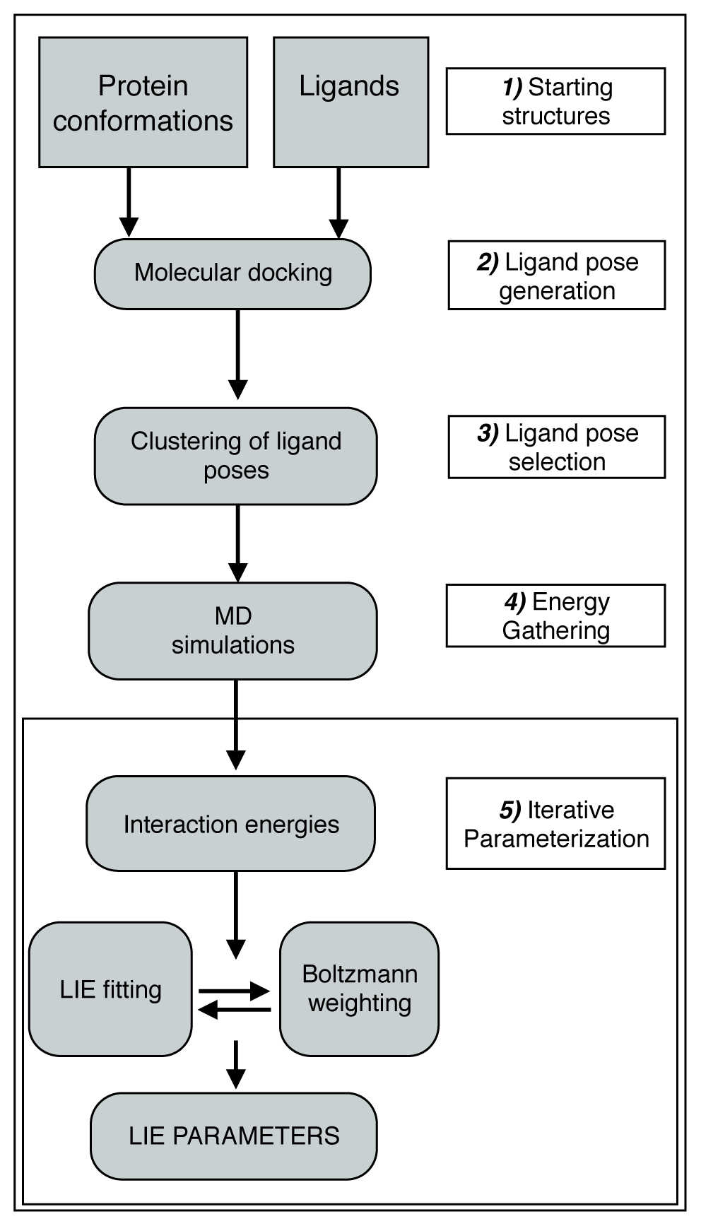
2.1. Automated Training
2.2. Automated Free Energy Prediction
2.3. Computational Details
2.3.1. Selection of Protein Conformations
2.3.2. Docking Procedure
2.3.3. Clustering
2.3.4. MD Simulations
3. Results and Discussion
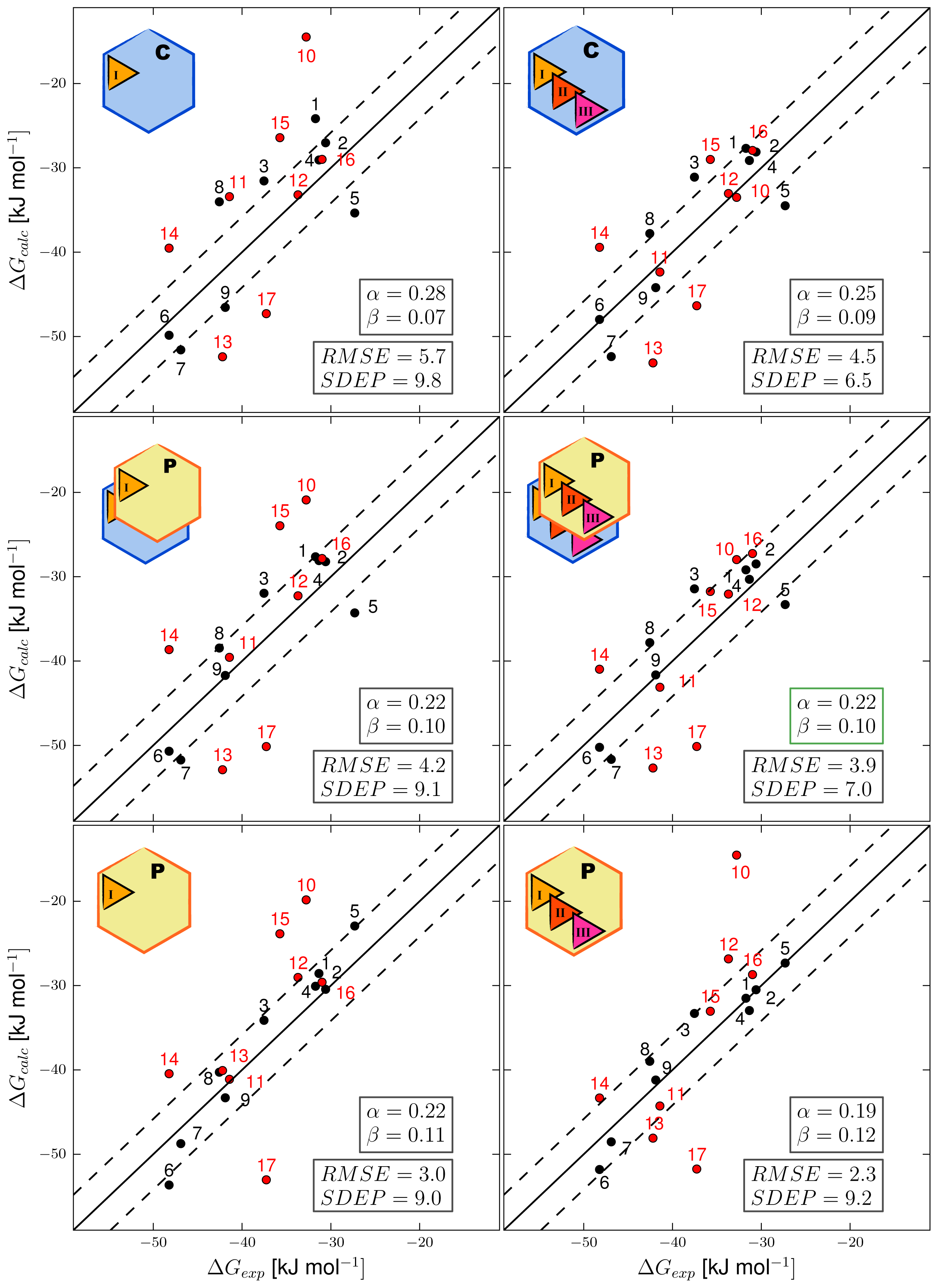
3.1. Automated Binding Free Energy Prediction
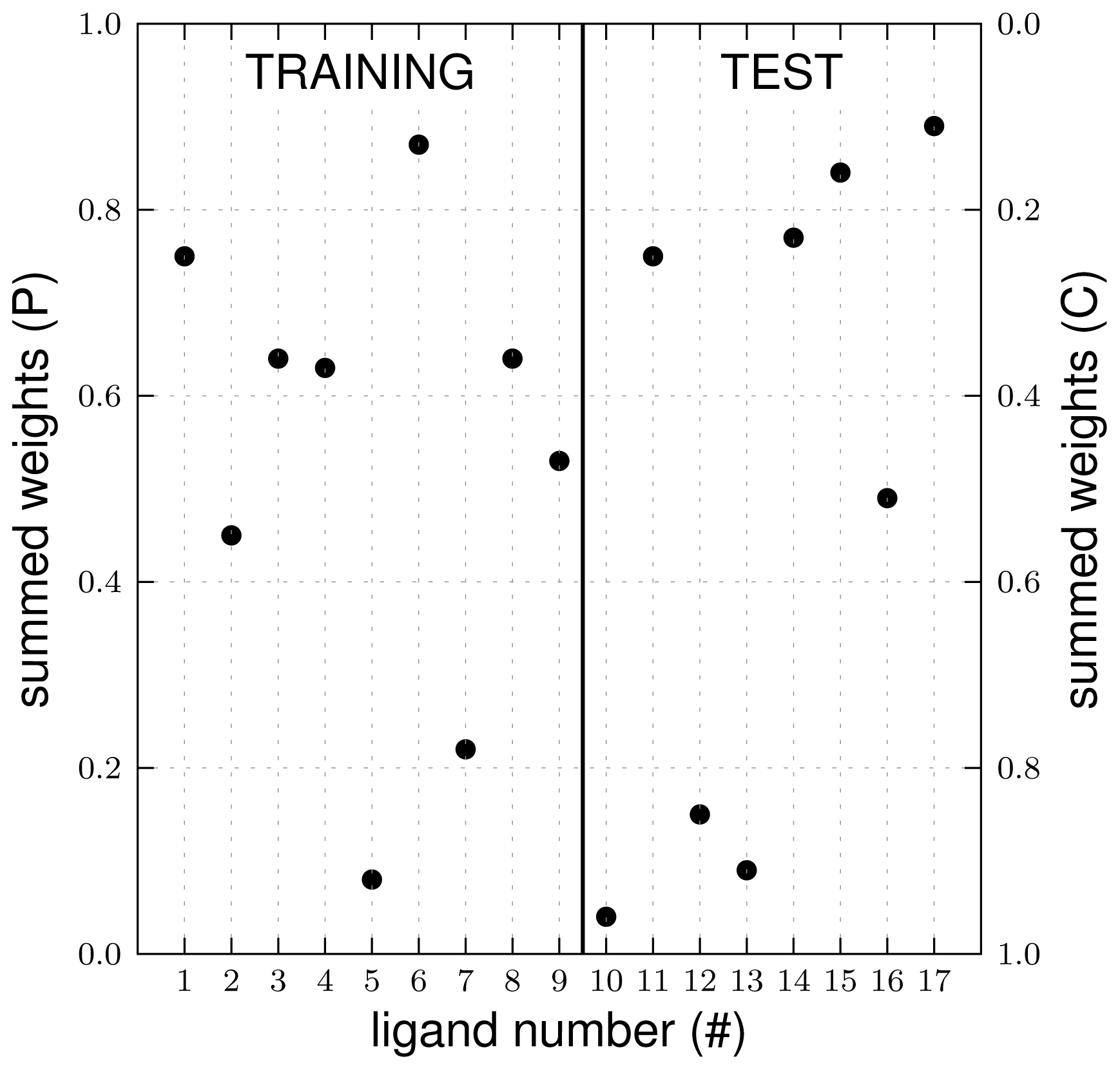
3.2. Assessing the Predictive Quality of the LIE Models
4. Conclusions
Supplementary Information
ijms-15-00798-s001.pdfAcknowledgments
Conflicts of Interest
References
- Chodera, J.D.; Mobley, D.L.; Shirts, M.R.; Dixon, R.W.; Branson, K.; Pande, V.S. Alchemical free energy methods for drug discovery: Progress and challenges. Curr. Opin. Struct. Biol 2011, 21, 150–160. [Google Scholar]
- Parenti, M.D.; Rastelli, G. Advances and applications of binding affinity prediction methods in drug discovery. Biotechnol. Adv 2012, 30, 244–250. [Google Scholar]
- De Graaf, C.; Oostenbrink, C.; Keizers, P.H.J.; van Vugt-Lussenburg, B.M.A.; Commandeur, J.N.M.; Vermeulen, N.P.E. Free energies of binding of R- and S-propranolol to wild-type and F483A mutant cytochrome P450 2D6 from molecular dynamics simulations. Eur. Biophys. J 2007, 36, 589–599. [Google Scholar]
- Stjernschantz, E.; Vermeulen, N.P.E.; Oostenbrink, C. Computational prediction of drug binding and rationalisation of selectivity towards cytochromes P450. Expert Opin. Drug Metab. Tox 2008, 4, 513–527. [Google Scholar]
- Kirchmair, J.; Williamson, M.J.; Tyzack, J.D.; Tan, L.; Bond, P.J.; Bender, A.; Glen, R.C. Computational prediction of metabolism: Sites, products, SAR, P450 enzyme dynamics, and mechanisms. J. Chem. Inf. Model 2012, 52, 617–648. [Google Scholar]
- Ortiz de Montellano, P. Cytochrome P450: Structure, Mechanism, and Biochemistry, 3rd ed; Kluwer Academic/Plenum Publishers: New York, NY, USA, 2005. [Google Scholar]
- Van Gunsteren, W.F.; Bakowies, D.; Baron, R.; Chandrasekhar, I.; Christen, M.; Daura, X.; Gee, P.; Geerke, D.P.; Glaettli, A.; Huenenberger, P.H.; et al. Biomolecular modeling: Goals, problems, perspectives. Angew. Chem. Int. Ed 2006, 45, 4064–4092. [Google Scholar]
- Rastelli, G.; Rio, A.D.; Degliesposti, G.; Sgobba, M. Fast and accurate predictions of binding free energies using MM-PBSA and MM-GBSA. J. Comput. Chem 2010, 31, 797–810. [Google Scholar]
- Klebe, G. Virtual ligand screening: Strategies, perspectives and limitations. Drug Discov. Today 2006, 11, 580–594. [Google Scholar]
- Christ, C.D.; Mark, A.E.; van Gunsteren, W.F. Basic ingredients of free energy calculations: A review. J. Comput. Chem 2010, 31, 1569–1582. [Google Scholar]
- De Ruiter, A.; Oostenbrink, C. Free energy calculations of protein–ligand interactions. Curr. Opin. Chem. Biol 2011, 15, 547–552. [Google Scholar]
- Guengerich, F. Cytochrome P450s and other enzymes in drug metabolism and toxicity. AAPS J 2006, 8, E101–E111. [Google Scholar]
- Stjernschantz, E.; Oostenbrink, C. Improved ligand-protein binding affinity predictions using multiple binding modes. Biophys. J 2010, 98, 2682–2691. [Google Scholar]
- Aqvist, J.; Medina, C. A new method for predicting binding affinity in computer-aided drug design. Protein Eng 1994, 7, 385–391. [Google Scholar]
- Perić-Hassler, L.; Stjernschantz, E.; Oostenbrink, C.; Geerke, D.P. CYP 2D6 binding affinity predictions using multiple ligand and protein conformations. Int. J. Mol. Sci 2013, 14, 24514–24530. [Google Scholar]
- Hritz, J.; Oostenbrink, C. Efficient free energy calculations for compounds with multiple stable conformations separated by high energy barriers. J. Phys. Chem. B 2009, 113, 12711–12720. [Google Scholar]
- Rastelli, G.; Degliesposti, G.; del Rio, A.; Sgobba, M. Binding estimation after refinement, a new automated procedure for the refinement and rescoring of docked ligands in virtual screening. Chem. Biol. Drug Des 2009, 73, 283–286. [Google Scholar]
- Hritz, J.; de Ruiter, A.; Oostenbrink, C. Impact of plasticity and flexibility on docking results for cytochrome P450 2D6: A combined approach of molecular dynamics and ligand docking. J. Med. Chem 2008, 51, 7469–7477. [Google Scholar]
- Vasanthanathan, P.; Olsen, L.; Jørgensen, F.S.; Vermeulen, N.P.E.; Oostenbrink, C. Computational prediction of binding affinity for CYP1A2-ligand complexes using empirical free energy calculations. Drug Metab. Dispos 2010, 38, 1347–1354. [Google Scholar]
- Stjernschantz, E.; Marelius, J.; Medina, C.; Jacobsson, M.; Vermeulen, N.P.E.; Oostenbrink, C. Are automated molecular dynamics simulations and binding free energy calculations realistic tools in lead optimization? An evaluation of the Linear Interaction Energy (LIE) method. J. Chem. Inf. Model 2006, 46, 1972–1983. [Google Scholar]
- Daura, X.; van Gunsteren, W.F.; Mark, A.E. Folding-unfolding thermodynamics of a β-heptapeptide from equilibrium simulations. Prot. Struct. Funct. Bioinf 1999, 34, 269–280. [Google Scholar]
- Keller, B.; Daura, X.; van Gunsteren, W.F. Comparing geometric and kinetic cluster algorithms for molecular simulation data. J. Chem. Phys 2010, 132, 074110. [Google Scholar]
- Wang, J.; Wang, W.; Kollman, P.A.; Case, D.A. Automatic atom type and bond type perception in molecular mechanical calculations. J. Mol. Graph. Model 2006, 25, 247–260. [Google Scholar]
- Malde, A.K.; Zuo, L.; Breeze, M.; Stroet, M.; Poger, D.; Nair, P.C.; Oostenbrink, C.; Mark, A.E. An automated force field topology builder (ATB) and repository: Version 1.0. J. Chem. Theory Comput 2011, 7, 4026–4037. [Google Scholar]
- Vanommeslaeghe, K.; MacKerell, A.D. Automation of the CHARMM General Force Field (CGenFF) I: Bond perception and atom typing. J. Chem. Inf. Model 2012, 52, 3144–3154. [Google Scholar]
- Vanommeslaeghe, K.; Raman, E.P.; MacKerell, A.D. Automation of the CHARMM General Force Field (CGenFF) II: Assignment of bonded parameters and partial atomic charges. J. Chem. Inf. Model 2012, 52, 3155–3168. [Google Scholar]
- Vaz, R.J.; Nayeem, A.; Santone, K.; Chandrasena, G.; Gavai, A.V. A 3D-QSAR model for CYP2D6 inhibition in the aryloxypropanolamine series. Bioorg. Med. Chem. Lett 2005, 15, 3816–3820. [Google Scholar]
- Yung-Chi, C.; Prusoff, W.H. Relationship between the inhibition constant (KI) and the concentration of inhibitor which causes 50 per cent inhibition (IC50) of an enzymatic reaction. Biochem. Pharmacol 1973, 22, 3099–3108. [Google Scholar]
- Caliper Online Product Database. Available online: http://www.caliperls.com/products/cyp2d6-h.htm (accessed on 20 August 2013).
- Eldridge, M.; Murray, C.; Auton, T.; Paolini, G.; Mee, R. Empirical scoring functions: I. The development of a fast empirical scoring function to estimate the binding affinity of ligands in receptor complexes. J. Comput. Aided Mol. Des 1997, 11, 425–445. [Google Scholar]
- Jones, G.; Willett, P.; Glen, R.C.; Leach, A.R.; Taylor, R. Development and validation of a genetic algorithm for flexible docking. J. Mol. Biol 1997, 267, 727–748. [Google Scholar]
- Schmid, N.; Christ, C.D.; Christen, M.; Eichenberger, A.P.; van Gunsteren, W.F. Architecture, implementation and parallelisation of the GROMOS software for biomolecular simulation. Comput. Phys. Commun 2012, 183, 890–903. [Google Scholar]
- Lins, R.D.; Hünenberger, P.H. A new GROMOS force field for hexopyranose-based carbohydrates. J. Comput. Chem 2005, 26, 1400–1412. [Google Scholar]
- Berendsen, H.J.C.; Postma, J.P.M.; van Gunsteren, W.F.; Hermans, J. Intermolecular Forces; Reidel: Dordrecht, The Netherlands, 1981; pp. 331–338. [Google Scholar]
- Berendsen, H.J.C.; Postma, J.P.M.; van Gunsteren, W.F.; Di Nola, A.; Haak, J.R. Molecular-dynamics with coupling to an external bath. J. Chem. Phys 1984, 81, 3684–3690. [Google Scholar]
- Ryckaert, J.P.; Ciccotti, G.; Berendsen, H. Numerical integration of the cartesian equations of motion of a system with constraints: Molecular dynamics of n-alkanes. J. Comput. Phys 1977, 23, 327–341. [Google Scholar]
- Tironi, I.G.; Sperb, R.; Smith, P.E.; van Gunsteren, W.F. A generalized reaction field method for molecular dynamics simulations. J. Chem. Phys 1995, 102, 5451–5495. [Google Scholar]
- Heinz, T.N.; van Gunsteren, W.F.; Hunenberger, P.H. Comparison of four methods to compute the dielectric permittivity of liquids from molecular dynamics simulations. J. Chem. Phys 2001, 115, 1125–1136. [Google Scholar]


| Ligand number # (# in Vaz et al.) | Structure | Properties |
|---|---|---|
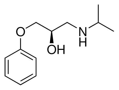
| 1 (6) |  | IC50 = 18 μM ΔGexp = −31.73 kJ mol−1 M = 210.30 g mol−1 q = +1e |
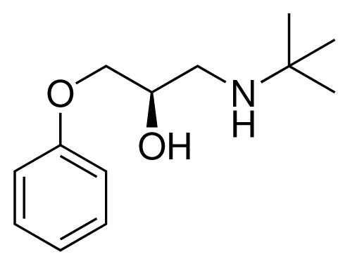
| 2 (10) |  | IC50 = 28 μM ΔGexp = −30.59 kJ mol−1 M = 224.32 g mol−1 q = +1e |
| 3 (7) |  | IC50 = 1.9 μM ΔGexp = −37.53 kJ mol−1 M = 260.36 g mol−1 q = +1e |
| 4 (3) |  | IC50 = 21 μM ΔGexp = −31.34 kJ mol−1 M = 266.36 g mol−1 q = +1e |
| 5 (8) |  | IC50 = 100 μM ΔGexp = −27.31 kJ mol−1 M = 317.41 g mol−1 q = +1e |
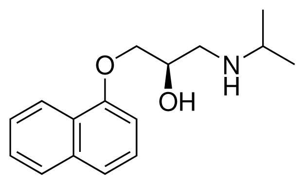
| 6 (5) |  | IC50 = 0.03 μM ΔGexp = −48.22 kJ mol−1 M = 389.52 g mol−1 q = +1e |
| 7 (26) |  | IC50 = 0.05 μM ΔGexp = −46.90 kJ mol−1 M = 382.46 g mol−1 q = +1e |
| 8 (22) |  | IC50 = 0.28 μM ΔGexp = −42.56 kJ mol−1 M = 404.60 g mol−1 q = +1e |
| 9 (28) |  | IC50 = 0.35 μM ΔGexp = −41.89 kJ mol−1 M = 417.55 g mol−1 q = +1e |
| Ligand number # (# in Vaz et al.) | Structure | Properties |
|---|---|---|
| 10 (19) |  | IC50 = 12 μM ΔGexp = −32.78 kJ mol−1 M = 435.52 g mol−1 q = 0e |
| 11 (12) |  | IC50 = 0.42 μM ΔGexp = −41.42 kJ mol−1 M = 394.50 g mol−1 q = +1e |
| 12 (16) |  | IC50 = 8.4 μM ΔGexp = −33.70 kJ mol−1 M = 290.38 g mol−1 q = +1e |
| 13 (18) |  | IC50 = 0.31 μM ΔGexp = −42.20 kJ mol−1 M = 380.47 g mol−1 q = +1e |
| 14 (14) |  | IC50 = 0.03 μM ΔGexp = −48.22 kJ mol−1 M = 339.46 g mol−1 q = +1e |
| 15 (4) |  | IC50 = 3.80 μM ΔGexp = −35.74 kJ mol−1 M = 273.38 g mol−1 q = +1e |
| 16 (9) |  | IC50 = 24 μM ΔGexp = −30.99 kJ mol−1 M = 268.38 g mol−1 q = +1e |
| 17 (20) |  | IC50 = 2.10 μM ΔGexp = −37.27 kJ mol−1 M = 464.59 g mol−1 q = +1e |
© 2014 by the authors; licensee MDPI, Basel, Switzerland This article is an open access article distributed under the terms and conditions of the Creative Commons Attribution license (http://creativecommons.org/licenses/by/3.0/).
Share and Cite
Vosmeer, C.R.; Pool, R.; Van Stee, M.F.; Perić-Hassler, L.; Vermeulen, N.P.E.; Geerke, D.P. Towards Automated Binding Affinity Prediction Using an Iterative Linear Interaction Energy Approach. Int. J. Mol. Sci. 2014, 15, 798-816. https://0-doi-org.brum.beds.ac.uk/10.3390/ijms15010798
Vosmeer CR, Pool R, Van Stee MF, Perić-Hassler L, Vermeulen NPE, Geerke DP. Towards Automated Binding Affinity Prediction Using an Iterative Linear Interaction Energy Approach. International Journal of Molecular Sciences. 2014; 15(1):798-816. https://0-doi-org.brum.beds.ac.uk/10.3390/ijms15010798
Chicago/Turabian StyleVosmeer, C. Ruben, René Pool, Mariël F. Van Stee, Lovorka Perić-Hassler, Nico P. E. Vermeulen, and Daan P. Geerke. 2014. "Towards Automated Binding Affinity Prediction Using an Iterative Linear Interaction Energy Approach" International Journal of Molecular Sciences 15, no. 1: 798-816. https://0-doi-org.brum.beds.ac.uk/10.3390/ijms15010798