Article

Comparison and Sensibility Analysis of Warning Parameters for Rotating Stall Detection in an Axial Compressor

CNRS, ONERA, Arts et Metiers Institute of Technology, Centrale Lille, University of Lille, UMR 9014—LMFL—Laboratoire de Mécanique des Fluides de Lille—Kampé de Fériet, F-59000 Lille, France
*
Author to whom correspondence should be addressed.
Int. J. Turbomach. Propuls. Power 2020, 5(3), 16; https://0-doi-org.brum.beds.ac.uk/10.3390/ijtpp5030016
Submission received: 22 April 2020 / Revised: 12 June 2020 / Accepted: 3 July 2020 / Published: 7 July 2020

Abstract

:
The present paper aims at evaluating the surveillance parameters used for early stall warning in axial compressors, and is based on unsteady pressure measurements at the casing of a single stage axial compressor. Two parameters—Correlation and Root Mean Square (RMS)—are first compared and their relative performances discussed. The influence of sensor locations (in both radial and axial directions) is then considered, and the role of the compressor’s geometrical irregularities in the behavior of the indicators is clearly highlighted. The influence of the throttling process is also carefully analyzed. This aspect of the experiment’s process appears to have a non-negligible impact on the stall warning parameters, despite being poorly documented in the literature. This last part of this research work allow us to get a different vision of the alert parameters compared to what is classically done in the literature, as the level of irregularity that is reflected by the magnitude of the parameters appears to be an image of a given flow rate value, and not a clear indicator of the stall inception.

Graphical Abstract

1. Introduction

Despite decades of development and improvement [1], axial compressors still lack rigorous design rules regarding rotating stall and surge [2]. Instead, aeroengines manufacturers apply consequent empirical security margins by considering the worst scenarios possible, to stay away from the stability limit whereat the compressor is subjected to transient events (inlet distortion, object ingestion, strong acceleration, etc.). This leads to limitations in the operating range of the engine, resulting in a lower pressure ratio and consequently a bigger engine, which induces higher drag and more weight for the aircraft.
Early detection of the stall phenomenon is thus an important part of the research work carried out by the scientific community. This task is particularly difficult in most of the modern compressors for which the transition to the unstable regime is sudden and fast. Another practical problem concerns the physical implementation of the sensors. Indeed, besides the lack of internal space (limiting the measurement means available), one must consider the optimal position of the sensors in order to get reliable information. Unsteady pressure measurements at casing are commonly applied to this purpose, thanks to the reliability of the sensors and their small size. Several studies can be found in the literature using data from pressure sensors to predict the rotating stall, but with varying methods. Some of them are based on a spectral analysis of pressure signals [3,4,5], by looking at the evolution of the frequency content in order to detect the apparition of modal oscillations. However, these methods are ineffective in the case of spike type rotating stall (see [6,7] for example). Today, the spike type rotating stall is the most common form of rotating stall observed in multistage compressors, because the critical incidence at the tip is often reached before the maximum of the total-to-static performance curve (see Day [2]). Thus, a popular choice among recent works, thanks to its relative simplicity, consists of tracking the loss of periodicity of the unsteady pressure profiles, due to the unsteadiness of the flow pattern close to the stability limit.
This technique, firstly spotted in the work of Inoue et al. [8], tracks the loss of periodicity using a cross-correlation of the instantaneous pressure signal at the casing with an unperturbed reference signal. This technique was then developed by Tahara et al. [9], then Dhingra et al. [6,10,11], to be finally applied to a full-scale engine by Christensen et al. [12]. More recently, Young et al. [13] proposed a slightly different method by computing the Root Mean Square (RMS) of the difference between the actual pressure signal at the casing and a reference. They also pointed out some limitations of the method in the presence of eccentricity.
Both solutions, correlation and RMS calculations, seem promising regarding a potential deployment on a real industrial system. However, to the knowledge of the authors, there is no study comparing these two solutions on an identical test bench, in order to achieve a real comparison and to highlight their respective limits. Besides, the influence of the compressor being brought to unstable operating conditions on the performance of these indicators has only been minimally considered.
To clarify these points, the present paper focuses on three topics:
The comparison of the behavior of these two indicators based on pressure signals obtained in near-stall operating conditions in a single stage axial flow compressor.
The effect of the sensor’s location on the evolution of these parameters, in order to determine an optimal location for the sensing system, will be then examined. In fact, despite being discussed by other authors in previous studies (Tahara et al. [14] or Young et al. [13]), some points are still subjected to debate, like for example the axial position of the sensors or the negative effect of the eccentricity.
The influence of the throttling process on the development of the rotating stall, and thus, on the evolution of the parameters.

2. Materials and Methods

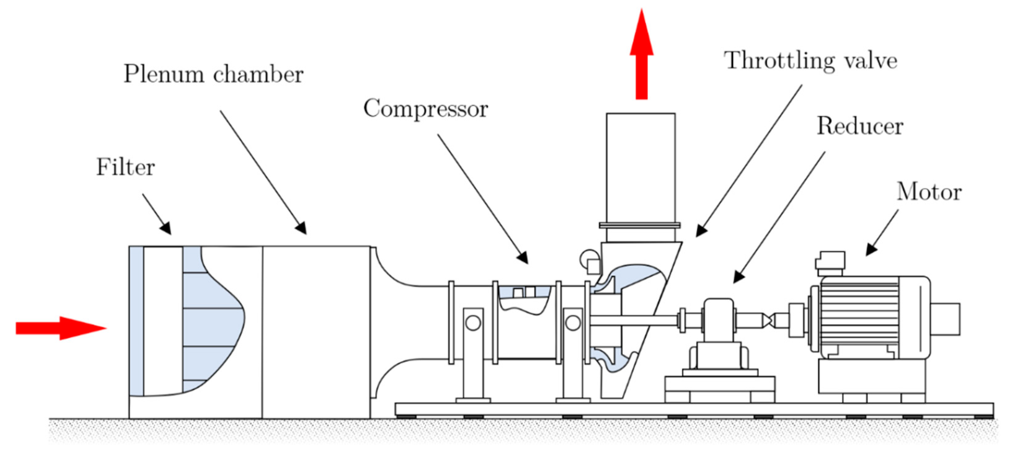
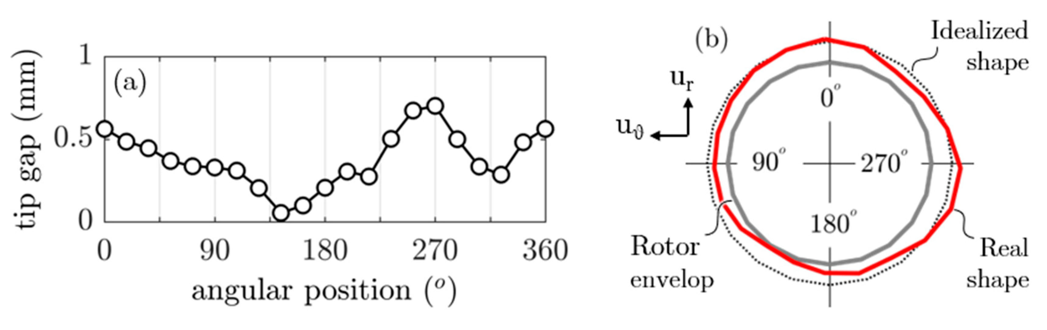
2.1. Experimental Setup

The experimental work presented in this paper has been realized on the single stage low pressure axial compressor CME2, composed of a 30-blades rotor and a 40-vanes stator. An overview of the test rig is proposed in Figure 1, and the main characteristics of the compressor are listed in Table 1. In this study, the compressor has been operated at a fixed rotational speed of 3200 r/min. At this speed the nominal flow rate is 5.3 kg·s−1.
In Figure 2, the reader can find the corresponding performance curve of the compressor, where the flow coefficient Φ = Vx/Umid is plotted as a function of the total-to-static pressure rise coefficient Ψt−s = ΔPt−s/(0.5ρU2mid). The design operating point of the compressor is marked by the black diamond (the other points will be explained in Section 2.2). As the slope of the characteristic suggests, the compressor is tip-critical and enters into the rotating stall through spike type inception (see Camp and Day [15]). This first observation has been confirmed by the absence of modal activities and the presence of a short-wavelength, high-amplitude perturbation a few revolutions before stall (as already shown by Veglio et al. [16]).
The measurements presented in this paper were realized with unsteady pressure transducers (Endevco model 8507C-1 and 8510B-1, MEGGITT, Coventry, UK), flush mounted on the casing and distributed all over the rotor. For this study, up to 20 transducers were used simultaneously following three specific patterns, showed in Figure 3, and listed hereafter:
  • For the first one, 20 transducers were non-evenly distributed at the same axial position (x/Cx = −0.06) to refine the sensor ring, and thus to have access to a more precise monitoring of the perturbations, in different regions, but also to take into account geometrical disparities (eccentricity, casing surface defect, etc.). Each location is represented by a red dot on Figure 3a;
  • For the second one, at four angular locations, 12 transducers were positioned over three axial positions [x/Cx = (−0.06; 0.55; 1.06)]. At a fifth angular position, eight more sensors were placed every 6 mm, to refine the discretization in the axial direction from just upstream of the leading edge (LE) to mid-chord. Each location is respectively represented by a blue diamond (12 sensors) and a green triangle (8 sensors) on Figure 3b.
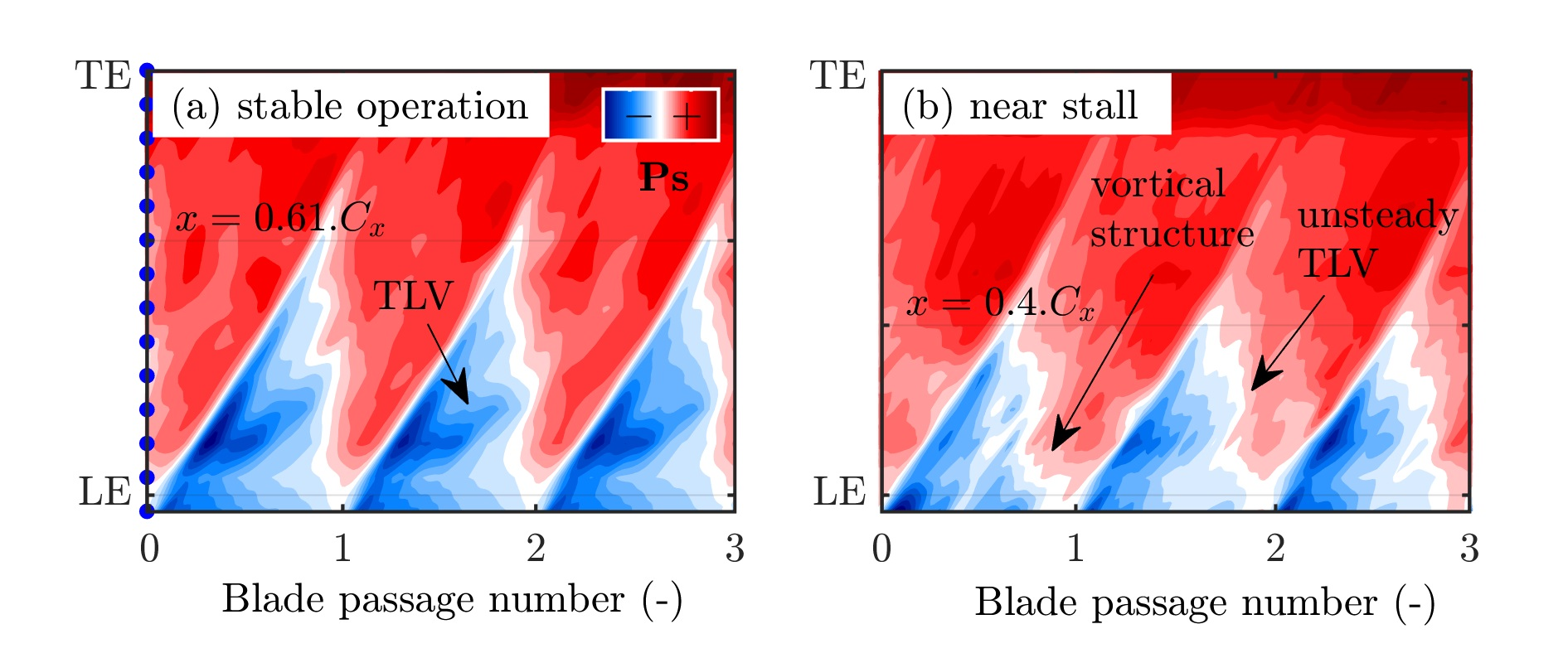
  • The third one has been solely used to analyze pressure contours from leading edge to trailing edge with enough accuracy at different operating points. For that purpose, 14 sensors, 4 mm apart, have been used. Their location is depicted on Figure 3c.
In configuration 2, the five locations of the first ring, x/Cx = −0.06 (visible in the radial view of Figure 3b), are common with configuration 1. During all the tests, the sampling rate was set to 100 kHz, corresponding to more than 60 measurement points on each blade channel at 3200 r/min, allowing us to catch perturbations of small temporal and spatial qualities. The pressure transducer’s uncertainty ranges from 0.5% to 1.5% of the full-scale output.

2.2. Experimental Procedure

As stated before, the effect of the throttling process on the evolution of the warning parameters is one of the interests motivating this study. The throttling process consists of reducing the mass flow rate going through the compressor in order to move the operating point from stable condition (green triangle on Figure 2) to unstable region (red circles “1” or “2” on Figure 2). Two methods have been investigated. Both are schematized on Figure 4:
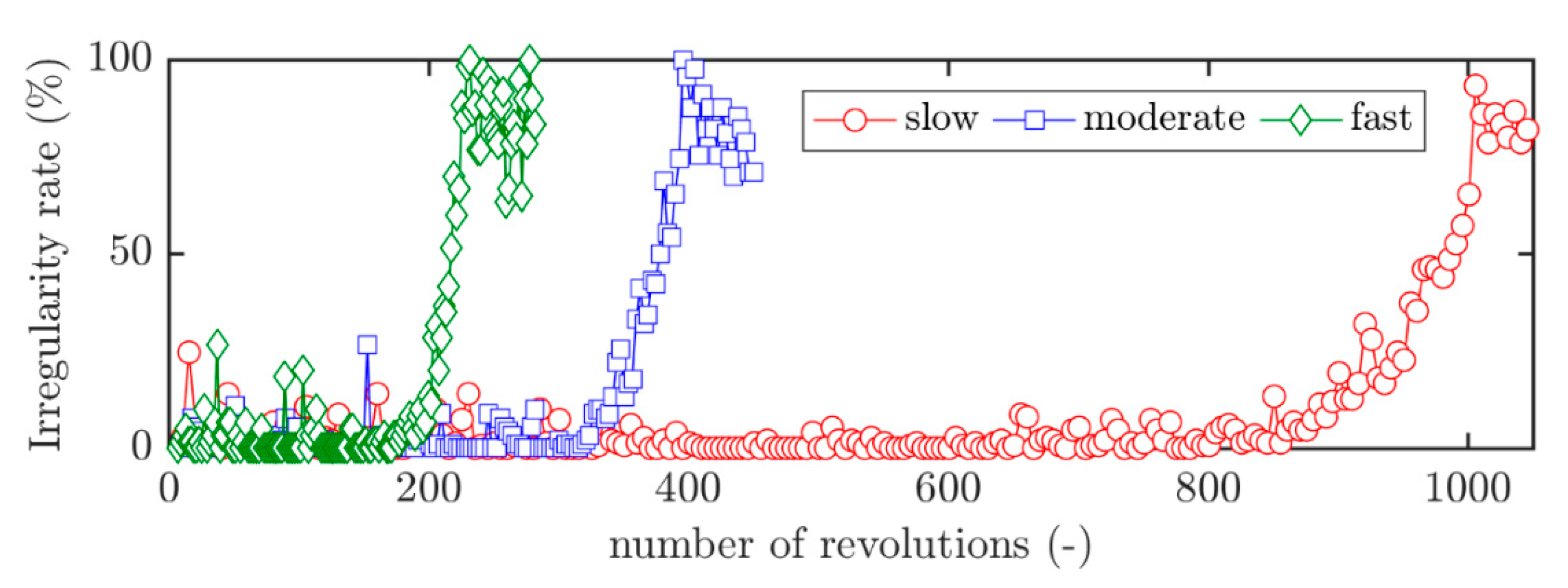
  • The first one corresponds to a complete throttling. For this procedure, the mass flow rate is decreased continuously until the rotating stall appears (red circle “2”). Three rates of decrease have been investigated, respectively equal to 0.30, 0.17, and 0.06 kg·s−2, and labelled fast, moderate and slow throttling speed in the following. The decrease rate of the mass flow rate is depicted in a previous article (see [17]). In this case, the rotating stall onset is forced;
  • The second one corresponds to partial throttling. In this case, the process is stopped just before the onset of the rotating stall, at the last stable operating point (red circle “1”), by a mechanical stop. The compressor continues to operate until it enters stall, or not. In this procedure, the rotating stall is spontaneous.
Each throttling process and throttling speed has been repeated 30 times, equally divided between both transducers pattern. Otherwise, the moderate speed has been tested 90 times in order to verify the convergence of the results.

2.3. Stall Warning Parameters

As stated in the Introduction, the first goal of this study is to compare two warning parameters proposed in the literature. Both are based on the same idea of comparing instantaneous blade passage pressure profiles to a reference profile. The difference is thus quantified by computing the Zero Normalized Cross-Correlation (labelled as C and simply referred to as Correlation in the following) or the Normalized Root Mean Square Deviation (labelled and referred to as RMS in the following). The expressions of these parameters are given in Equations (1) and (2):
C ( t ) = 1 2 ( 1 i = 1 wnd P ref ( i ) × P ( t + i ) i = 1 wnd P ref ( i ) 2 × i = 1 wnd P ( t + i ) 2 )
RMS ( t ) = i = 1 wnd ( P ref ( i ) P ( t + i ) ) 2 i = 1 wnd P ref ( i ) 2 + i = 1 wnd P ( t + i ) 2
To simplify the comparison obtained with the two parameters, they are both scaled so that (i) they both return 0 if the instantaneous signal is exactly the same as the reference signal, and (ii) they both return 1 if the instantaneous signal and the reference signal present a phase shift of 180°.
In these expressions, P(t + i) refers to the instantaneous blade passage pressure signal, Pref(i) to the reference pressure profile, wnd being the size of the temporal window used to perform the computation, which is the duration between two subsequent blade passages in this study.
Two definitions of Pref(i) can be considered:
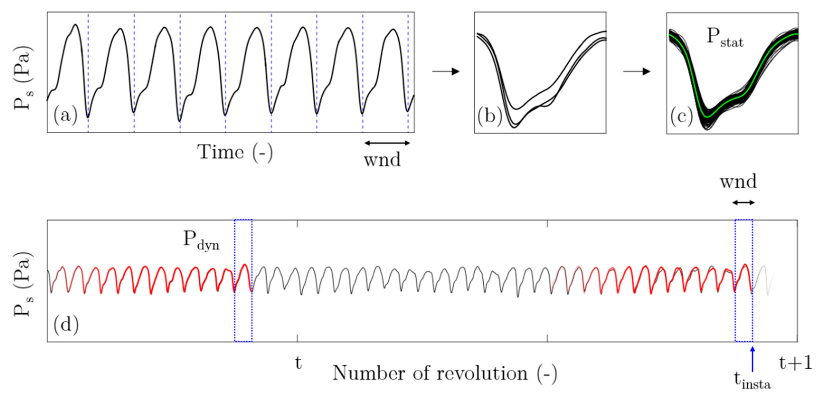
  • The simplest one would be to choose a reference profile calculated by averaging several blade pressure signatures obtained from several revolutions (five, in the results presented in the paper) at a stable operating point. This reference profile will be referred to as Pstat, and is similar to the procedure used by Young et al. [13].
  • The second one consists of a sliding reference profile, equal to a single passage, extracted one revolution before the one being evaluated. Unlike the latter, it is thus computed at each time step of the throttling process and evolves all along the test. This reference profile will be referred to as Pdyn and is similar to the procedure used by Christensen et al. [12] or Tahara et al. [14].
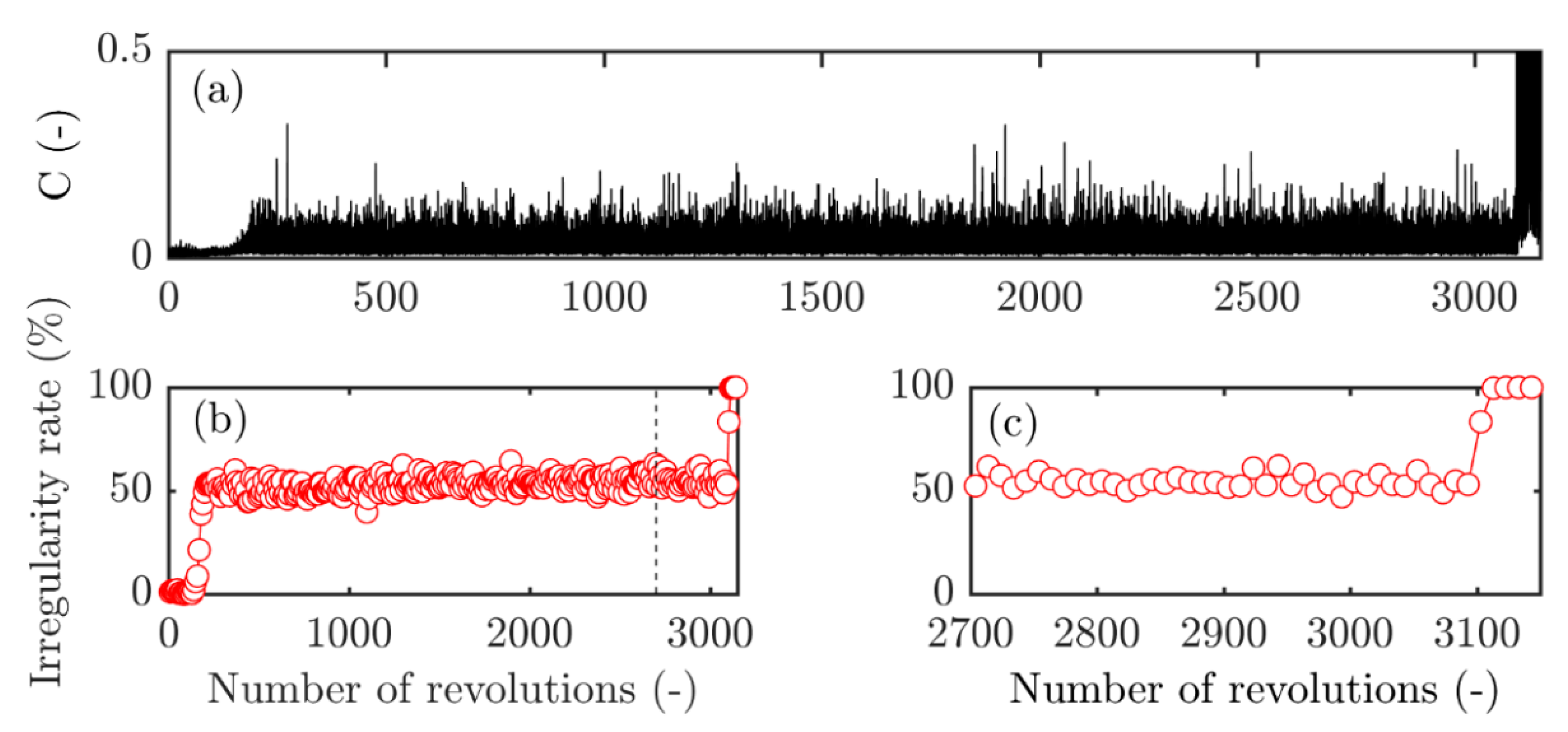
A schematic representation of both profiles is depicted in Figure 5.
In compressors, the flow is expected to be fully turbulent, presenting thus random fluctuations of its physical properties, including pressure. One expects then some important variations of the instantaneous values of the parameters (see Figure 6a). A possible solution for a practical application of these two parameters is to proceed to a statistical treatment of the data, by analyzing the percentage of sufficiently perturbed profiles during a given period. A profile is thus defined as perturbed (yellow dots in Figure 6c,d) when the surveillance parameter value crosses a given threshold (red dotted line in Figure 6a). By calculating the proportion of perturbed profiles against the total number of profiles over a given period, we then obtain a percentage of perturbed profiles, which that can be tracked over time and which is displayed in Figure 6e. In the following, the percentage of perturbed profiles, computed over 5 revolutions, will be referred to as irregularity rate, and will be used in future works as the driving parameter for a control system (Figure 6e).
When no specification is given, the Correlation and the RMS will be referred to as surveillance parameters since their goal is to monitor the pressure measurements and to quantify the instantaneous pressure irregularity.
The use of a threshold to discriminate the state of a pressure profile thus implies that its value is clearly determining. If it is too low, every profile will be considered perturbed. If it is too high, the irregularity rate will ramp up too close to the stall onset. Moreover, the shape of the profile can also change during the life of the compressor due to the aging of its components (eccentricity, tip gap size change, blades wear), or can be affected by vibrations of the system itself (support bearing, housing, etc.). This irregularity rate can also be affected by axisymmetric irregularities (casing shape, flow distortion), thus depending on the position of the sensor, but this question will be addressed later in the paper. To take into account these dependencies and to define an appropriate threshold value, an automatic optimization procedure has been used to “objectively” set up the threshold. This method is based on the distribution of the values taken by the surveillance parameters (i.e., Correlation or RMS) during stable operations. Figure 7a shows, for example, a typical result, for a given test, of the cumulative distribution, Fc, of the correlation every 5 revolutions. This function is defined as follow:
F C ( x ) =   ( C ( t ) x c )
where C(t) is the value of the Correlation at instant t, and ( C ( t ) x c ) the probability of the Correlation of a given pressure profile being lower than the value xc.
On this plot, each function represents the distribution of each correlation value xc, as a percentage of the total number of values over the period (here equal to 5 revolutions × 30 pitches = 150). In this figure, the shape of the cumulative distributions changes as the compressor is pushed toward stall. Up to 250 revolutions, where the compressor still operates in the stable region, all the distributions exhibit similar shapes. One observes in particular that the maximum values of the distribution (i.e., Fc = 100%) are very close. The evolution of the value under which falls 100% of the instantaneous correlation is plotted in Figure 7b. By taking the mean value during stable operation (up to 250 revolutions), one can easily obtain the value of the surveillance parameter for which, on average, 100% of the profiles are considered healthy. Then, this value can be used to set up the threshold to discriminate normal profiles from perturbed ones. In the case presented in Figure 7b, this threshold will be fixed to 0.012. This value is automatically adjusted for each test, surveillance parameter and sensor location.

3. Results

3.1. Dynamic vs. Static Reference Profile

The choice of the reference pressure profile does not affect both surveillance parameters equally. During the throttling process, two different phenomena can affect the general shape of all the pressure profiles: (i) when the operating point approaches the stability limit, the amplitude of the pressure fluctuations increases (Figure 8a); and (ii) some unsteady phenomena (vortical structures, boundary layer separation) can affect a limited number of profiles. The warning procedure described in the previous section aims to catch the occurrence of the second type of profile modification, as they are the trace of phenomena that can trigger the transition to rotating stall. Since the RMS computes the direct difference between both signals, when used with the reference profile Pstat its values show an increase as soon as the throttling process starts, as depicted in Figure 8d. In this case, the surveillance parameter increase mainly reflects the modification of the amplitude of the instantaneous profile. The Correlation exhibits the same behavior, to a smaller extent, as shown in Figure 8b. Indeed, this parameter is normalized by the autocorrelation of each signal, and computes a difference in the shape of the signals, which exhibits not as many changes when the amplitude increases.
On the other hand, when a dynamic reference profile is used (Figure 8c,e), the modification of the general shape of the profile does not affect the surveillance parameter, which increases only with the unsteadiness of the flow (in the last hundreds of revolution, in Figure 8c). Consequently, in the following, for both surveillance parameters (RMS or Correlation), the dynamic reference pressure profile has to be preferred. It will then referred to only as the reference profile, noted Pref in the following.

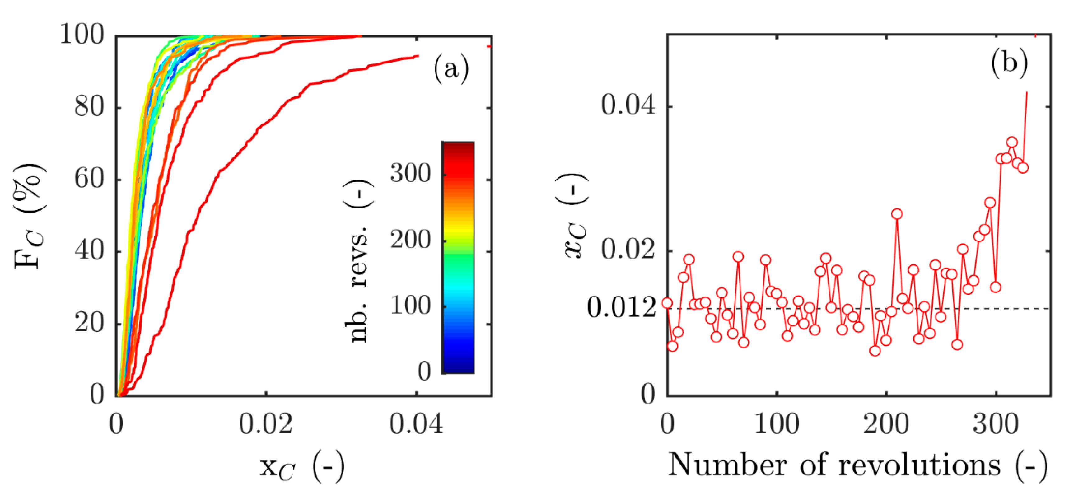
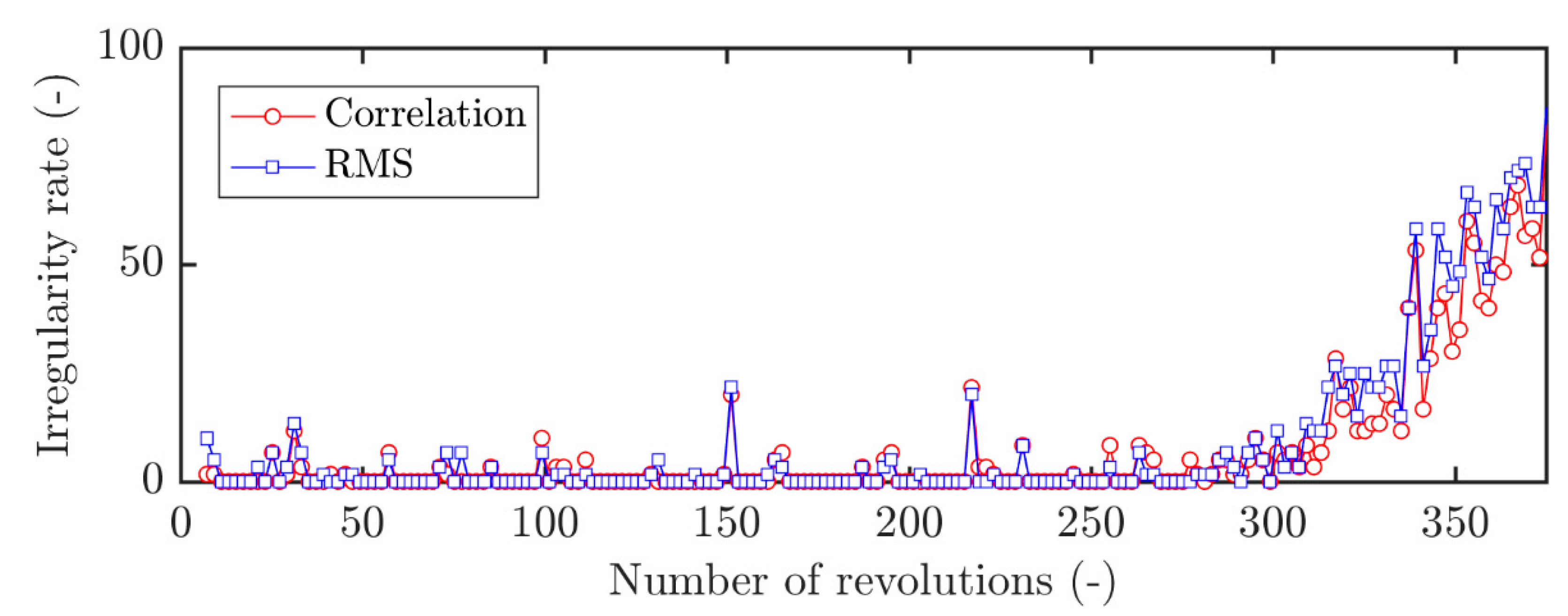
3.2. Comparison of Surveillance Parameters

The procedure used to determine the value of the threshold to apply in order to obtain the best irregularity rate provides an efficient way to compare both surveillance parameters. Indeed, the irregularity rate is thus computed in a manner similar to the Correlation and the RMS, allowing thereby an objective comparison.
The evolution of this irregularity is computed for both surveillance parameters, and displayed in Figure 9 for a representative test.
On this figure, the irregularity rates computed from both surveillance parameters stay around 0% at the beginning, and both start increasing at the same time with the same trend. This behavior was also observed for the other tests, whatever the location of the sensor or the throttling speed. The difference in the evolution of the two curves, from a global standpoint, thus seems negligible.
This lack of differences was further investigated through handmade artificial signals (rounded sawtooth waveform), representative of the blade passing pressure signature. For the sake of clarity, as this part of the study does not change the above-mentioned statement, only its main conclusions are presented here. They add some shades to this apparent lack of difference.
This artificial pressure signal, similar to the blade signature, was first superimposed with various level of white noise, and then used to compute both surveillance parameters. The first difference was identified here, as the Correlation appears to be much more efficient in detecting irregularities in the presence of random perturbations than the RMS. In other words, Correlation appears to have a slightly better signal to noise ratio.
Another difference arises when superimposing higher frequency pulses (i.e., perturbation wavelength smaller than a blade pitch) on each blade signature with different phase shifts (i.e., negative or positive pressure perturbations at different angular locations in the blade pitch), as displayed in Figure 9a. It appears that if the RMS performs consistently no matter the location of the perturbation (see Figure 9b), the Correlation returns lower values when the sign of the perturbation is the same as the local trend (i.e., positive perturbation on positive slope of the blade pressure signature, and correspondingly negative on negative). In other words, a low-pressure perturbation, like a radial vortex, will be better captured by the Correlation if it is located in the high-pressure region of the blade passage when passing in front of the sensor.
However, as depicted in Figure 10, these local differences totally disappear from a global standpoint, when the irregularity rate is used, because a threshold is applied on the parameter. Indeed, this irregularity rate monitors the number of perturbed profiles, and not their actual level of irregularity. The difference of Correlation due to the position of the perturbation thus has no impact as long as the lowest score is higher than the threshold. The reader is thus advised to keep this behavior in mind when using the Correlation. From the perspective of the application considered in the paper, both surveillance parameters appear to perform equally. Consequently, in the following sections, only results concerning the Correlation will be presented, but the results obtained can be generalized to the RMS.

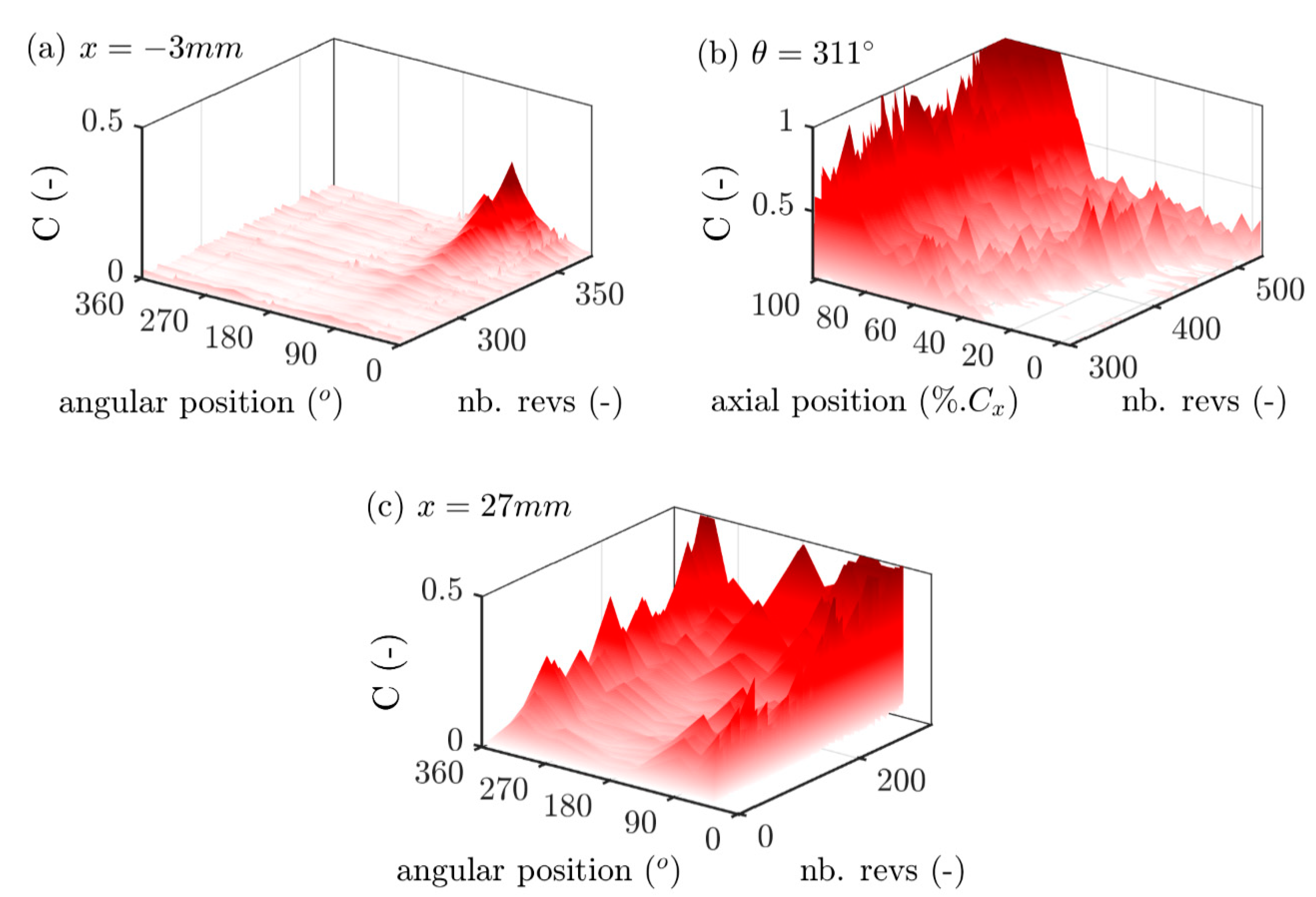
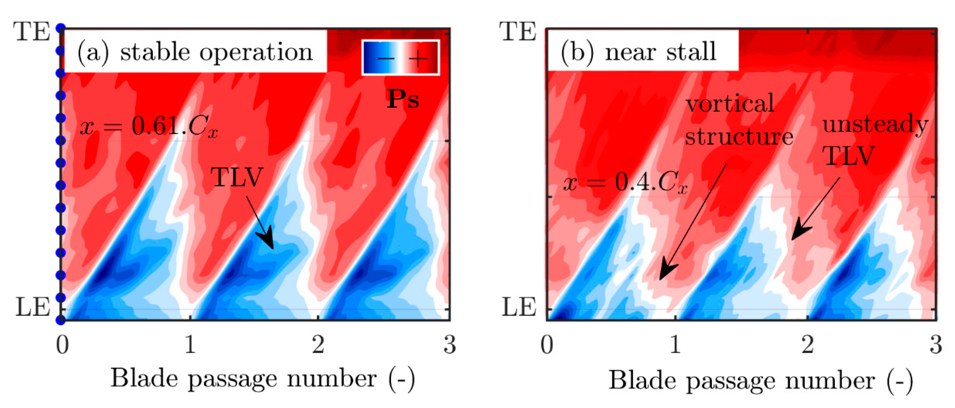
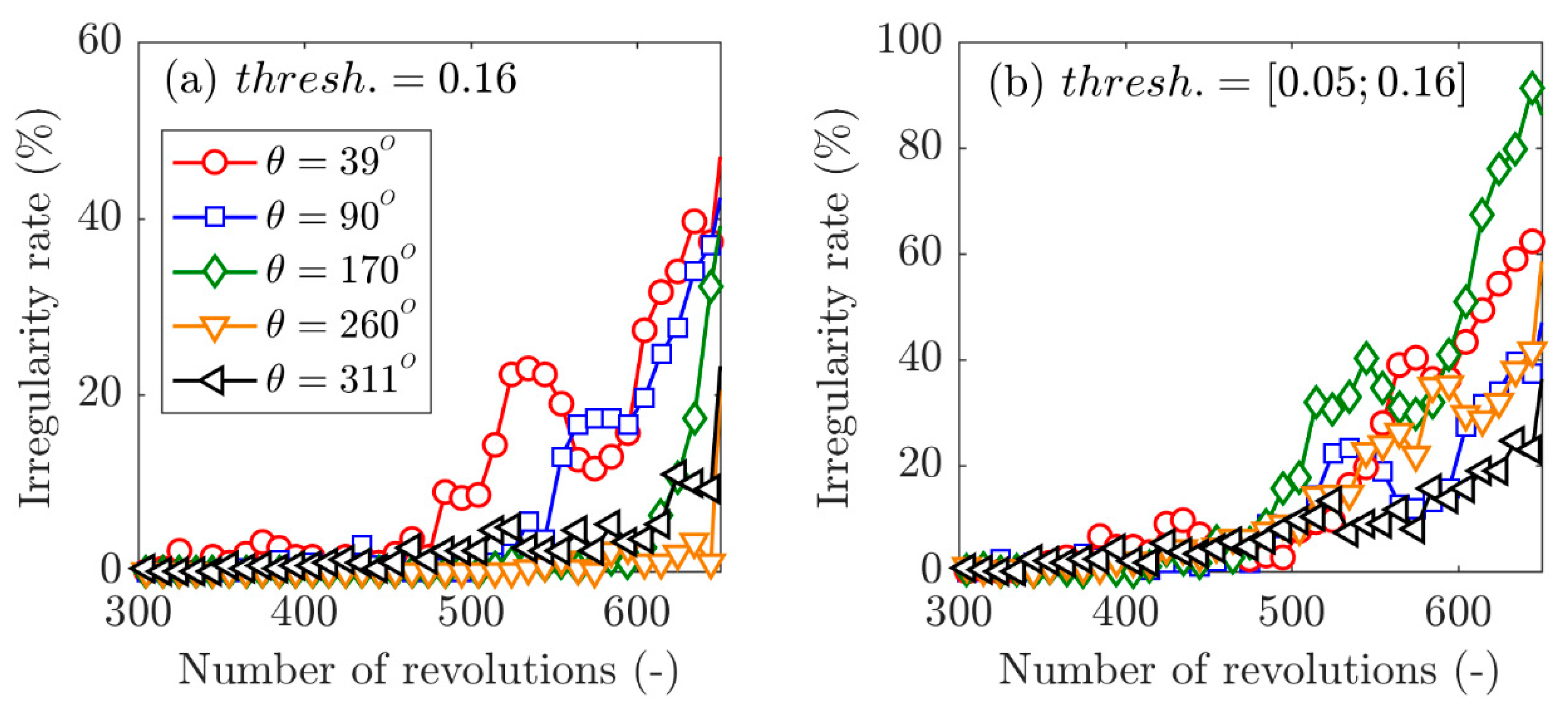
3.3. Influence of Sensor Location

The evolution of the surveillance parameters at different axial and angular locations is now investigated.
To do so, the evolution of the Correlation has been analyzed over 20 angular locations (presented in Figure 3a) (covering the whole circumference) for x = −0.06Cx, 14 axial positions (ranging from the leading edge to the trailing edge of the rotor) for θ = 311°, and five angular positions for x = 0.55Cx (Figure 3b). The results have been gathered on Figure 11.
Before analyzing these results, it is important to have in mind the “true shape” of the compressor casing. Several profiles of the casing have been measured with a contact probe at different axial locations before the experiments. This profile, depicted in Figure 12, exhibits a slightly oval shape with a reduction of the gap in the 0°–100° and 250°–300° sectors.
On Figure 11a, one can clearly see that the Correlation displays a strong degradation around θ = 90°. This confirms the findings of Young et al. [13], who showed that the degradation of the surveillance parameter was observed in the region where the gap varies from large to small values. Using the Graf model (Graf et al. [18]), they showed that the compressor will be locally less stable in the large tip gap sector due to a lower local flow coefficient. This loss of stability appears with a slight offset compared to the maximum value of tip clearance, and will promote rotating stall onset in those regions. They have also linked this loss of stability to the presence of prestall disturbances in this particular region. This behavior has been confirmed in the present setup, with a rotating stall onset rate of 73% in the region directly after the maximum value of tip clearance. It can be noted however on Figure 11a that no degradation is observable in the 270°–300° sector, when it should be according to the Graf model, which also works for two-lobed asymmetry. The assumption made here to explain this difference is the presence of a not-captured eccentricity of the rotor in the 250° direction. Indeed, for the record, only the shape of the casing has been measured.
In Figure 11b, we can see, firstly, that the further downstream a transducer is from the leading edge, the greater the degradation of the warning parameter is, and the sooner it appears. When the operating point moves closer to the stability limit, several phenomena occur. The low-pressure zone attached to the suction side shrinks in the axial direction. This behavior is clearly visible on Figure 13. In this figure, two pressure contours, extracted at a stable operating point (a) and near the stability limit (b), are presented. The sensors’ locations, depicted in Figure 3c, can be seen on the y-axis of Figure 13a. One can see that the size of the low-pressure zone decreases from 61% of the axial chord to 40%, in the axial direction. A second behavior is also visible on this figure where the Tip Leakage Vortex (TLV) can only be easily distinguished from the stable operating points (Figure 13a). When the operating point approaches the stability limit, the TLV decreases in size and becomes highly unsteady. The apparition of vortical structures is also visible close to the leading edge. All these phenomena explain why the degradation of the Correlation is earlier for downstream positions. However, for positions further than x = 0.5Cx, the Correlation does not exhibit noticeable degradation over time. Indeed, the events detected by the Correlation (low-pressure zone shrinkage, TLV destabilization, radial vortices, etc.) are localized in the first half of the chord. In addition to this lack of features to detect, the pressure signals are more perturbed and do not allow a reliable detection.
Thus, Figure 11c also focuses on the degradation of the Correlation for different angular positions, at the axial position x = 0.55Cx. The correlation displays here a strong degradation for every angular position, but still presents the asymmetry visible earlier around θ = 90°. However, this asymmetry is far less pronounced for this downstream location, and all angular positions display at least some degradation before the rotating stall onset, unlike upstream positions.
Thus, axial locations in the first half of the channel are more suitable than locations upstream of the leading-edge. Even for the non-axisymmetric tip gap, there will be an axial location where the surveillance parameter will display a degradation. To overcome the non-even distribution of correlation degradation, it is however necessary to adapt the threshold value depending on the sensor angular position. This can be realized thanks to the automatic optimization procedure presented earlier, and an example is presented in Figure 14. In Figure 14a, the same threshold is applied whatever the sensor location, and as expected, the irregularity rate starts increasing at different moments, ranging from t = tstall—200 revolutions to t = tstall—0 revolutions. In Figure 14b, however, the threshold is changed from one sensor to the other, which leads to almost simultaneous degradation of the irregularity rate. It can also be noted that the slope of the irregularity rate is different depending on the angular position. Indeed, the procedure proposed here only allows one to consider the perturbed profile sooner by analyzing the “normal” level of perturbation under stable operating conditions, and therefore only impacts the irregularity rate degradation at the beginning. However, the quantity of irregularity creations during the throttling remains circumscribed to the local flow and tip gap, thus explaining the difference in slope.
In addition to compensating for the geometrical disparities, such automatic optimization procedure can also be, presumably, well suited to compressor aging. As suggested by Young et al. [13], the geometrical features of a compressor change constantly during the life of the engine, which will therefore induce different levels of irregularity. This geometrical change should be covered by this procedure.

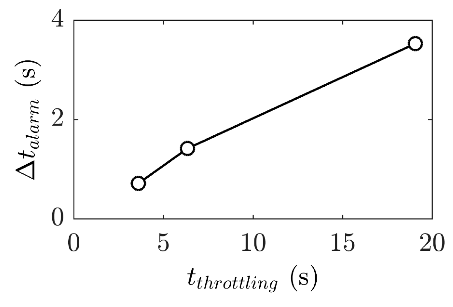
3.4. Influence of the Throttling Process

In this section, we look at the influence of the throttling process on the evolution of the Correlation and the irregularity rate. Both complete and partial throttling are addressed. Some of the results concerning the first process have been presented in a previous paper [17], and are recapitulated here.
Figure 15 depicts the time evolution of the irregularity rate during a complete throttling, for the three throttling speeds. It can be clearly seen that the faster the operating point moves toward the stability limit, the faster the irregularity rate increases.
To confirm this qualitative observation, the average time between the moment the irregularity rate becomes higher than 50% and the rotating stall onset, referred as Δtalarm, is defined. This time is plotted on Figure 16 as a function of the characteristic time of the throttling speed, tthrottling, defined as the time necessary to reduce the flow rate from 4.75 to 4.25 kg·s−1 (this range has been conveniently chosen as the middle of the throttling range). Figure 16 clearly shows that Δtalarm varies inversely proportionally to the throttling speed.
Figure 17 presents the evolution of the surveillance parameter and the associated irregularity rate, during a partial throttling procedure in a representative test. The end of the throttling procedure is reached around t = 200 revolutions, and after this point, the compressor continues working properly during almost 3000 revolutions. [It should be noted that this duration is totally random from one test to the other, ranging from a few hundred (i.e., a few seconds) to several thousand revolutions (i.e., a few minutes).] Whether thousands of revolutions (Figure 17b) before stall or just a few (Figure 17c), the irregularity rate shows no evolution of any kind, and remains around 50%. This lack of evolution of the irregularity rate at this last stability point indicates an absence of noticeable degradation of the flow in the tip region.
This last result confirms that the level of irregularity is, if not an image of the degradation of the flow that leads to the stall, at least an image of the position of the operating point. Indeed, when the throttling is stopped just before stall, no further degradation arises, thus showing a link between the position of the operating point and the irregularity rate. The ultimate degradation only happens when the operating point crosses the stability limit, and is materialized by a jump in irregularity at t = 3100 revolutions on Figure 17c.
This is a quite unexpected and surprising result, compared with the current knowledge about stall inception monitoring. In fact, with it being just an image of the instantaneous flow rate, one can argue that basing a warning parameter on it could be quite risky, and useless in the case of a quick shift of the operating point toward the stability limit. However, a clever application of this finding would be to use it as a true image of the current operating point, and then as a “level of risk” as regards the onset of the rotating stall.

4. Discussion

The performances of two surveillance parameter definitions (i.e., Correlation and RMS) available in the literature have been evaluated, based on unsteady pressure measurements realized on the casing of a single-stage axial flow compressor test bench. A new method to automatically choose the relevant threshold needed to practically apply both surveillance parameters proposed in the literature is offered. This method could be especially useful to compensate for some eventual degradation of the surveillance parameter due to an increase of irregularities over the life of a gas turbine. The two surveillance parameters are based on the comparison of instantaneous pressure profiles to a reference one. This reference profile can be static (fixed during the whole procedure) or dynamic. It has been shown that a static reference is not suited to irregularities measurement, because it records any small change of the operating point, whereas dynamic ones only exhibit degradation close to the stability limit.
RMS- and Correlation-based parameters have been compared. Despite exhibiting some minor differences, it appears that the threshold detection methods make them perform equally well in irregularity rate monitoring. Taken independently, however, the Correlation returns a different level of irregularity depending on the position of the perturbations inside the pressure profile. This behavior, not detrimental in the present case, must be taken into account. Moreover, calculation costs were not investigated in the current study, and could be a convenient way to choose one or the other of these two surveillance parameters.
The influence of the location of the sensors was then investigated. As shown in the literature, the surveillance parameter, close to the leading edge, presents a strong dependency on the tip gap size. However, in light of the present work, these conclusions must be nuanced, as the surveillance parameter exhibits changing behaviors depending on the axial location in the blade passage. In the first half of the passage, the eccentricity dependency is less prominent, and all angular positions exhibit a degradation before stall. Thus, it would be wise, on a real application, to place the pressure sensors in this area in order to overcome the detrimental influence of the tip gap size on the evolution of the parameter. These observations also mitigate the questioning proposed by other authors concerning the real utility of irregularity measurement methods in real applications.
The last series of tests, conducted with different throttling processes, highlighted that the performance of the surveillance is directly linked to the throttling process. More precisely, the warning time between the reaching of a given irregularity rate and the onset of the stall is inversely proportional to the speed of the throttling, in the case of a complete throttling. In the case of a throttling process stopped at an operating point close to stall, the surveillance parameters remain at a constant value, on average, throughout the whole time the compressor operates at this operating point, until stall onset. It appears that the surveillance parameter is not an indicator of flow irregularities that could trigger stall, but is instead an image of the instantaneous flow rate.
This study has brought to the gas turbine community a convenient method for implementing a stall detection algorithm, taking into account practical aspects like geometrical features (imperfections or shape modifications during the compressor’s lifetime), sensor positioning and “objective” parameter setup. However, this is only one of the many outcomes to be addressed in order to see, in the near future, a fully functional active stall control system, allowing us to reduce the stall margin in aeroengines.
In fact, once the stall proximity is detected, one has to act on the flow to prevent or delay it. Active flow control is a promising method, but many questions arise here: which flow structures have to be targeted to mitigate the stall phenomenon? What is the best kind of perturbation to inject into the main flow to do that? How does one guarantee the overall efficiency of the control action? Some of these questions have partial answers in the literature, while some others’ answers are still missing. The next step in the current research work of the authors is thus to refine and complete the available knowledge on the subject, in order to get both a better comprehension of the complex and unstable phenomena prior to stall, but also to consider high TRL experiments in order to contribute to the development of an industrial grade active stall control system able to “pay its place” on a commercial aircraft.

Author Contributions

Conceptualization, A.D.; Formal analysis, G.M..; Funding acquisition A.D. and O.R.; Investigation G.M.; Methodology G.M., P.J., A.D. and O.R., Project administration A.D. and O.R.; Software G.M.; Supervision A.D., P.J. and O.R.; Validation P.J.; Visualisation G.M.; Writing: original draft, G.M.; Writing: review and editing G.M., P.J., A.D. and O.R. All authors have read and agreed to the published version of the manuscript.

Funding

This research was funded by the ANR project NUMERICCS (ANR-15-CE06-0009).

Conflicts of Interest

The authors declare no conflict of interest. The funders had no role in the design of the study; in the collection, analyses, or interpretation of data; in the writing of the manuscript, or in the decision to publish the results.

Abbreviations

The following symbols and abbreviations are used in this manuscript:
CCorrelation
CxBlade axial chord (mm)
FcCumulative distribution function of the Correlation
LELeading edge
PdynDynamic reference pressure profile
PrefReference pressure profile
PstatStatic reference pressure profile
qMass flow rate (kg·s−1)
RMSRoot Mean Square Deviation
TLVTip Leakage Vortex
TRLTechnology Readiness Level
tthrottlingCharacteristic time of the throttling process (s)
UmidMean rotor speed (m·s−1)
urRadial direction
uxAxial direction
uθTangential direction
VxAbsolute axial velocity (m·s−1)
wndAnalyzed temporal window duration
xcArbitrary value of the Correlation
Xt−sTotal-to-static quantity
ΔPPressure rise (Pa)
ΔtalarmMean warning time (s)
ρAir density (kg·s−1)
ΦFlow coefficient, Φ = Vx/Ut
ΨPressure rise coefficient, Ψt−s = ΔPt−s/0.5ρUt2.
ωRotor rotational speed (r/min)

References

  1. Nichelson, B.J. Early Jet Engines and the Transition from Centrifugal to Axial Compressors: A Case Study in Technological Change; University of Minnesota: Saint Paul, MN, USA, 1988. [Google Scholar]
  2. Day, I.J. Stall, Surge, and 75 Years of Research. J. Turbomach. 2015, 138, 011001. [Google Scholar] [CrossRef]
  3. Paduano, J.D.; Epstein, A.H.; Valavani, L.; Longley, J.P.; Greitzer, E.M.; Guenette, G.R. Active Control of Rotating Stall in a Low-Speed Axial Compressor. J. Turbomach. 1993, 115, 48–56. [Google Scholar] [CrossRef]
  4. Haynes, J.M.; Hendricks, G.J.; Epstein, A.H. Active Stabilization of Rotating Stall in a Three-Stage Axial Compressor. J. Turbomach. 1994, 116, 226–239. [Google Scholar] [CrossRef]
  5. Tryfonidis, M.; Etchevers, O.; Paduano, J.D.; Epstein, A.H.; Hendricks, G.J. Pre-Stall Behaviour of Several High-Speed Compressor. In Proceedings of the International Gas Turbine and Aeroengine Congress and Exposition, Orlando, FL, USA, 3–6 July 1994. [Google Scholar]
  6. Dhingra, M.; Neumeier, Y.; Prasad, J.V.R.; Breeze-Stringfellow, A.; Shin, H.-W.; Szucs, P.N. A Stochastic Model for a Compressor Stability Measure. J. Eng. Gas Turbines Power 2006, 129, 730–737. [Google Scholar] [CrossRef]
  7. Höss, B.; Leinhos, D.; Fottner, L. Stall Inception in the Compressor System of a Turbofan Engine. J. Turbomach. 2000, 122, 32–44. [Google Scholar] [CrossRef]
  8. Inoue, M.; Kuroumaru, M.; Iwamoto, T.; Ando, Y. Detection of a Rotating Stall Precursor in Isolated Axial Flow Compressor Rotors. J. Turbomach. 1991, 113, 281–287. [Google Scholar] [CrossRef]
  9. Tahara, N.; Nakajima, T.; Kurosaki, M.; Ohta, Y.; Outa, E.; Nisikawa, T. Active stall control with practicable stall prediction system using auto-correlation coefficient. In Proceedings of the 37th Joint Propulsion Conference and Exhibit, Salt Lake City, UT, USA, 8–11 July 2001; American Institute of Aeronautics and Astronautics: Salt Lake City, UT, USA, 2001. [Google Scholar]
  10. Dhingra, M.; Neumeier, Y.; Prasad, J.V.R.; Shin, H.-W. Stall and Surge Precursors in Axial Compressors. In Proceedings of the 39th AIAA/ASME/SAE/ASEE Joint Propulsion Conference and Exhibit, Huntsville, AL, USA, 20–23 July 2003; American Institute of Aeronautics and Astronautics: Reston, VA, USA, 2003. [Google Scholar]
  11. Dhingra, M.; Armor, J.; Neumeier, Y.; Prasad, J.V.R. Compressor Surge: A Limit Detection and Avoidance Problem. In Proceedings of the AIAA Guidance, Navigation, and Control Conference and Exhibit, Austin, TX, USA, 5–8 August 2005; American Institute of Aeronautics and Astronautics: Reston, VA, USA, 2005. [Google Scholar]
  12. Christensen, D.; Cantin, P.; Gutz, D.; Szucs, P.N.; Wadia, A.R.; Armor, J.; Dhingra, M.; Neumeier, Y.; Prasad, J.V.R. Development and Demonstration of a Stability Management System for Gas Turbine Engines. J. Turbomach. 2008, 130, 031011. [Google Scholar] [CrossRef]
  13. Young, A.M.; Day, I.J.; Pullan, G. Stall Warning by Blade Pressure Signature Analysis. J. Turbomach. 2012, 135, 011033. [Google Scholar] [CrossRef]
  14. Tahara, N.; Kurosaki, M.; Ohta, Y.; Outa, E.; Nakajima, T.; Nakakita, T. Early Stall Warning Technique for Axial-Flow Compressors. J. Turbomach. 2007, 129, 448. [Google Scholar] [CrossRef]
  15. Camp, T.R.; Day, I.J. A Study of Spike and Modal Stall Phenomena in a Low-Speed Axial Compressor. In Volume 1: Aircraft Engine; Marine; Turbomachinery; Microturbines and Small Turbomachinery; ASME: Orlando, FL, USA, 1997; Volume 120, p. V001T03A109. [Google Scholar]
  16. Veglio, M.; Dazin, A.; Bois, G.; Roussette, O. Pressure Measurements in an Axial Compressor: From Design Operating Conditions to Rotating Stall Inception. In Proceedings of the 49th Symposium of Applied Aerodynamics, Lille, France, 24–26 March 2014. [Google Scholar]
  17. Margalida, G.; Dazin, A.; Joseph, P.; Roussette, O. Detailed Pressure Measurements During the Transition to Rotating Stall in an Axial Compressor: Influence of the Throttling Process. In Proceedings of the ASME 2018 5th Joint US-European Fluids Engineering Division Summer Meeting, Montreal, QC, Canada, 15–19 July 2018; p. V001T01A001. [Google Scholar]
  18. Graf, M.B.; Wong, T.S.; Greitzer, E.M.; Marble, F.E.; Tan, C.S.; Shin, H.-W.; Wisler, D.C. Effects of Nonaxisymmetric Tip Clearance on Axial Compressor Performance and Stability. J. Turbomach. 1998, 120, 648. [Google Scholar] [CrossRef] [Green Version]
Figure 1. CME2 axial compressor.
Ijtpp 05 00016 g001
Figure 2. Compressor performances.
Ijtpp 05 00016 g002
Figure 3. Pressure transducer locations.
Ijtpp 05 00016 g003
Figure 4. Schematic representation of the throttling process. (a) Complete throttling; (b) partial throttling.
Ijtpp 05 00016 g004
Figure 5. Construction of the reference profile. Static reference profile (ac); dynamic reference profile (d).
Ijtpp 05 00016 g005
Figure 6. Schematic representation of the evolution of the surveillance parameter and the warning parameter for a given surveillance threshold. (a) Surveillance parameter evolution during a test; (bd) zoomed views; (e) irregularity rate evolution.
Ijtpp 05 00016 g006
Figure 7. (a) Correlation cumulative distribution functions (computed over 5 revolutions and displayed every 20) as a function of the correlation value; (b) iso-level of distribution. Sensor location: (x,θ) = (−0.06.Cx, 90°); moderate throttling speed.
Ijtpp 05 00016 g007
Figure 8. Evolution of the surveillance parameters during a throttling process. (a) Time evolution of pressure; (b) Correlation—Static reference profile; (c) Correlation—dynamic reference profile; (d) RMS—Static reference profile; (e) RMS—dynamic reference profile. Sensor location: (x,θ) = (−0.06.Cx, 90°); moderate throttling speed.
Ijtpp 05 00016 g008
Figure 9. Effect of the position of a perturbation in the blade passage signature on the Correlation and RMS parameters. (a) Perturbed signal; (b) Correlation and RMS response.
Ijtpp 05 00016 g009
Figure 10. Irregularity rate evolution computed from the Correlation and the RMS (surveillance threshold respectively equal to 0.012 and 0.021). Sensor location: (x,θ) = (−0.06.Cx, 90°); moderate throttling speed.
Ijtpp 05 00016 g010
Figure 11. Correlation evolution during a throttling process. (a) For different angular positions, −0.06Cx upstream of the LE; (b) for different axial positions at θ = 311°; (c) different angular positions, 0.55Cx downstream of the LE.
Ijtpp 05 00016 g011
Figure 12. Evolution of the gap around the circumference of the compressor. (a) Tip gap size as a function of the angular position and (b) real shape of the casing.
Ijtpp 05 00016 g012
Figure 13. (a) Pressure contour during stable operation and (b) near stall. θ = 311°. Sensors are represented by blue dots.
Ijtpp 05 00016 g013
Figure 14. (a) irregularity rate evolution at five angular positions for a constant threshold and (b) optimized thresholds depending on the sensor location. x = 0.55Cx, moderate throttling speed.
Ijtpp 05 00016 g014
Figure 15. Evolution of the irregularity rate for three different throttling speeds.
Ijtpp 05 00016 g015
Figure 16. Evolution warning time Δtalarm as a function of tthrottling for the 3 continuous throttling speeds.
Ijtpp 05 00016 g016
Figure 17. Correlation and irregularity rate evolution for a fixed operating point just before stall. (a) Correlation; (b) irregularity rate; (c) zoomed view of the irregularity rate. Sensor location: (x,θ) = (−0.06Cx, 90°).
Ijtpp 05 00016 g017
Table 1. Compressor parameters.
Geometrical ParametersNon-Dimensional Operating Parameters
Tip diameter549 mmInlet axial Mach number0.12
Hub–tip ratio, LE0.75Flow coefficient, Φ0.44
Theoretical rotor tip gap0.5 mmTotal-to-static pressure rise coefficient0.45
Rotor chord84 mm
Rotor tip stagger angle54°

