1. Introduction
CFD continues to be a critical tool in the design and development of turbomachinery equipment. It is used in the evaluation of the performance of complex multistage turbines at design and off-design points, and in the optimization of single blades. Furthermore, the continuous increase in available computational resource has allowed for a substantial improvement in the quality of simulations as compared to a decade ago. While the majority of compressible flows still uses the perfect gas model, it is becoming more common to work on applications where real gas effects are no longer negligible. Example where these situations occur include low pressure stages of steam turbines [
1] or ORC turbines [
2].
Many authors have investigated the impact of various real gas models, mainly focusing on possible achievements in the accuracy of the results and the impact on computational time due to the increased complexity of the thermophysical models, see, e.g., [
2,
3,
4,
5,
6,
7]. The later point, the increase in computational time, has, however, received less attention. While the complexity of real gas relations is probably the most obvious cause, other factors also play a role, such as the iterative nature of the solution procedures used to update thermophysical properties. This non-linearity is often addressed by using lookup tables, see, e.g., [
5]. In this case the user needs to know in advance the range of the thermophysical states, which is not always available at the start of a simulation. This is further complicated by the fact that, prior to convergence, some intermediate solutions can run out of the tabulated range. For such situations, a stabilization criterion is needed. Additional issues arise concerning the resolution of the generated lookup table. A low resolution may lead to a faster numerical procedure, but can diminish the quality of the results. The high sensitivity of the results to lookup table resolution was described in [
8]. Other techniques to address the weakness of lookup tables include the use of structured grids for the lookup tables and the use of various interpolation methods whether bi-linear or bi-cubic ([
5]).
In this paper the real gas relations are incorporated algebraically, i.e., without using lookup tables, into an in-house, pressure based, all-speed, fully coupled solver [
9,
10,
11]. The main intention is therefore to contribute to the understanding of the necessary modifications considering a compressible all-Mach solver when using real gas state equations. Starting from the basic real gas relation, the conservation equations and boundary conditions and the derivation of the developed numerical techniques are presented in details with a main focus on retaining the performance and robustness of the coupled solver. Furthermore, the computational cost of the use of real gas relations is thoroughly investigated. Although the developed methods to deal with real gas relations are general, two specific relations are evaluated in more detail. It is for the reason that these models are later used for the validation and it is considered a contribution to help the reader to apply the procedure to his desired real gas model. The highlighted models are the cubic state equations, e.g., [
12] and the IAPWS database for water at any state [
13]. It will be shown that the increase in computational time often does not justify the problems arising from lookup table formulations. Replacement with tabulated data is, however, straight forward.
Three test cases are used to validate and evaluate the presented numerical approach. In the first case, the consistency of the approach is demonstrated. This is accomplished by showing that the solution of additional iterative procedures needed for real gas formulations recovers the results of the perfect gas model when applied to a 2D transonic bump case. In the second test case, the IAPWS-97 formulation [
13] is applied to a nozzle configuration with the operating range varying from supersonic to transonic flow regimes. The expansion for the transonic conditions yield to operating conditions in the two-phase region. Results are compared to those obtained from a commercial code. The last test case is an industrial type two stage compressor at one operational speed for the full range from choking flow to the stability limit, the cubic state equations are used as they are the manufacturer’s choice for this application. Results are then compared against measurement data. Furthermore, for cases two and three, an evaluation of the computational cost of the real gas implementations is presented.
2. Thermodynamic Modeling of Real Gas
Real gases are compositions of materials at thermophysical states under which its molecules are dense enough so that intermolecular forces can no longer be neglected. This is in contrast to the theory of ideal gases. For ideal gases, the molecules are sparsely distributed in space and these forces are not taken into account. It is this assumption that leads to the well known ideal gas state equation.
The fundamental derivative of gas dynamics is a key parameter in understanding real-gas flows. It is a measurement for the change in speed of sound through a change in density, its definition is provided in Equation (
1).
While this expression reduces to a constant value of for perfect gas and is always greater than one, this does not apply for real gas. A special example are Bethe–Zel’dovich–Thompson (BZT) fluids, which are heavy polyatomic compositions. For these materials, can even have negative values when approaching the critical point. The effect is an inverted gas dynamic behavior, where, contrary to perfect gas, the Mach number decreases as the flow expands.
2.1. General Comment on Real Gas Modeling
The modeling of real gases in a numerical framework is accompanied with a variety of additional challenges. This is a direct result of the increased complexity of the state equations compared to the simple ideal gas state equations. The non-linearities introduced require iterative updates of a variety of quantities, which will be a major part of what follows. It also requires a profound analysis of all underlying equations and thermophysical relationships. Entropy, internal energy and enthalpy are a function of two variables for the general case of a real gas. Since cubic equations are used in the final validation (in which ), the equations and partial derivatives are given using as primary input variable. However, this does not limit the generality of the approach and just requires a careful derivation of what is exemplified below. are interchangeable through the state equation, but depending on its formulation it may simplify the analysis if the input variables are changed to, e.g., .
2.2. Real Gas State Equations
Various models have been proposed to better account for intermolecular forces when encountering denser fluids, each having its own justification depending on the operting conditions and the working fluid. Analytical representation for superheated and two-phase steam is given by the model of Young [
14] in virial form or for water at any state in the form given through IAPWS [
13]. When modeling hydrocarbons, cryogenic fluids or refrigerants, well known virial equations are those of Benedict–Webb–Rubin (BWR) [
15] and its modifications. Another group of real gas state equations is represented in the form of cubic state equations. The original formulation was introduced by Van der Waals [
16] but many other models have emerged to overcome some of its drawbacks. Modifications have been applied to improve the phase transition, see Soave et al. [
17], or the prediction of liquid phase density and accuracy in the critical region by Peng et al. [
12].
2.2.1. Cubic State Equations
The cubic state equation, used for the final validation case, is based on the formulation provided by Peng et al. [
12] and therefore given in Equation (
2).
and
are temperature and pressure at the critical point and
being the accentric factor.
2.2.2. IAPWS-97
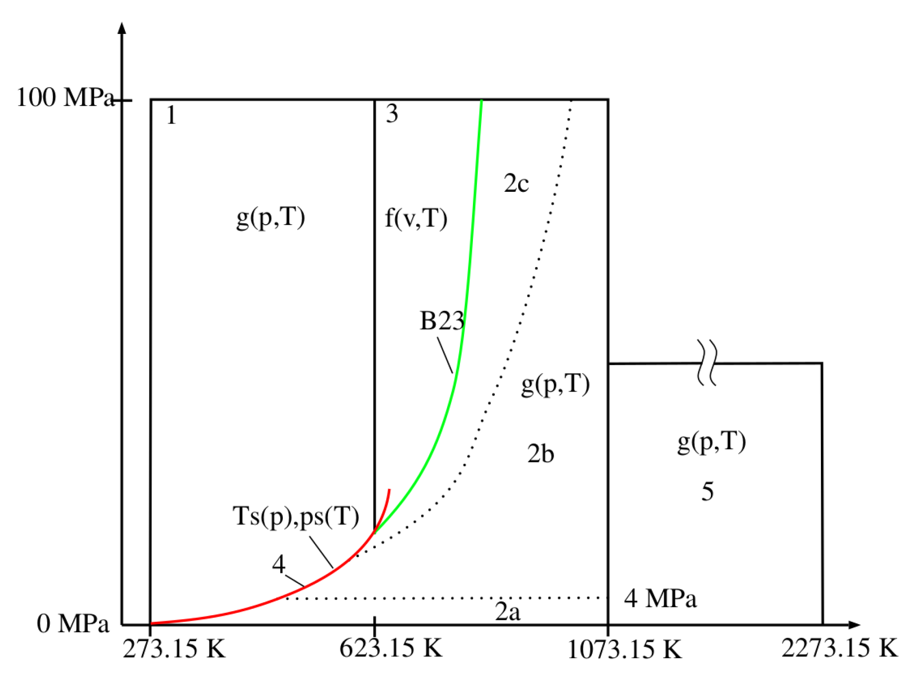
The IAPWS-97 [
13] formulations provide accurate state equations for the properties of water at any state. The equations are highly polynomial functions and provided for five different subregions described in
Figure 1. Region 1 is the liquid phase and region 3 accounts for the transition from liquid to gaseous phase above the critical point. Region 2 and 5 are gaseous states and region 4 is the two-phase region below the critical point.
While this set of equations allows for a highly accurate representation of the properties of water, they can lead to a massive increase in computational costs. Even by the use of provided backwards functions to eliminate at least partially the iterative procedures the increase in computational time is still considerable. The usual approach is therefore the use of lookup tables generated using IAPWS formulations.
2.3. Caloric State Equations and Definition of Entropy
The numerical algorithm requires values of internal energy, entropy and enthalpy at a certain point. This can be the case during the update of variables that are not a direct outcome of a conservation equation such as temperature or density. However, it may also be required when updating boundary conditions, such as given stagnation conditions at the inlet. Using real gas state equations, the definitions of the caloric state equations for enthalpy and internal energy are functions of two intensive properties, e.g., temperature and pressure, and are no longer only a function of temperature alone. The derivation of generalized state equations is therefore briefly described here on the basis of internal energy.
The definition for the change in internal energy is given in
Appendix A and the final expression is shown in Equation (
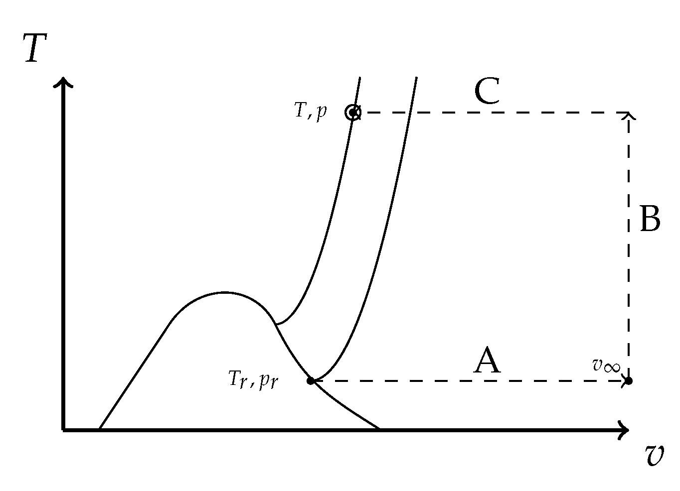
5). The integral form of this differential equation can be found using an integration along paths as shown in
Figure 2.
The value of
is computed through integration along lines of constant temperature (
) and constant specific volume (
B) using a given reference state
. The final expression for internal energy is thus given in Equation (
6), formulations for enthalpy and entropy (see
Appendix E) can be found using the same basic idea.
It is obvious that such a representation of the integral value can be understood as the sum of the ideal gas contribution plus a correction to adjust for real gas effects. As stated earlier, ideal gas behavior is encountered when intermolecular forces do not affect the properties of the fluid. This is always valid if the molecules are separated by an infinite distance. In other words the density goes towards zero or specific volume to infinity. Hence the integration along line
B accounts for the ideal gas contribution, and integration along the lines
corrects the value to correspond to the real gas change in the state variable. The ideal gas heat capacity in term
B can be described with a variety of models. The simplest is the assumption of calorically perfect gas (i.e.,
= const.), other options are Sutherland models or NASA’s polynomial approach [
18]. As stated in the introduction, the final validation of the coupled solution strategy for real gas CFD is based on an industrial sized two-stage radial compressor. It is the manufacturer’s choice to use the Peng–Robinson [
12] state equation.
Appendix C therefore gives a detailed derivation of Equation (
6) for this type of state equation. To provide an example of the generality of the approach the derivations for internal energy for the Benedict–Webb–Rubin (BWR) [
15] state equation are given in addition in
Appendix D.
2.4. Stagnation Conditions
Evaluation of stagnation conditions given static values or vice versa is a necessity frequently encountered in engineering practice. The relation is usually based on the assumption of an isentropic state change, leading to the well known expressions for incompressible and compressible (assuming ideal gas) flows as given in Equations (
7) and (
8) exemplarilly for pressure.
These relationships usually provide the basis in the derivation of stagnation conditions, however they do not apply to real gas. In the derivation of Equation (
8) it is assumed that the isentropic exponent is a constant, a simplification which is not valid for real gas. Some authors ([
19,
20]) argue that the variations are, however, small and Equation (
8) can be applied with minimal loss of accuracy. While this may be a justified assumption for a variety of applications, its generality is questionable. The generalized approach used in the present article is therefore explained in later sections when describing boundary conditions and the update of domain internal quantities.
2.5. Specific Heat Capacity
As already introduced when discussing the stagnation conditions, the heat capacity and heat capacity ratio do no longer follow the well known ideal gas relations. The heat capacity ratio can vary for different thermophysical states and requires a generalized approach. The derivation used in the implementation is therefore given in detail in
Appendix F. The final expression is given in Equation (
9)
2.6. Mach Number
The Mach number is a frequently used quantity for the post-processing and analysis of numerical results. In the following we will therefore provide a general formulation for the speed of sound. The definition of the Mach number is given by Equation (
10).
The speed of sound for any compressible medium is given by Equation (
11).
Detailed derivation of the partial differential of pressure with respect to density under isentropic conditions can be found in
Appendix G. The final expression is given in Equation (
12).
The partial differentials can again be found in
Appendix B.
3. Numerical Environment
Segregated pressure-based solution algorithms [
21,
22] based on the SIMPLE family of algorithms have been applied successfully over the past decades. The popularity of these algorithms is partly due to their low memory requirement based on the sequential method in solving the RANS equations. Another reason is the relatively simple implementation. On the downside, these algorithms suffer from convergence breakdown for large-scale problems. The reason for this issue is that the naturally strong pressure-velocity coupling is numerically decoupled when solving the momentum and continuity equation sequentially.
Owing to the developments in computer architecture, coupled solution strategies for pressure-based algorithms have regained interest in recent years [
23,
24]. These algorithms solve the momentum and continuity equation together, i.e., coupled. The numerical framework used in this article is based on the coupled solution strategy presented in [
9,
10,
11]. The coupled system of linearized momentum and continuity equations for each cell of the computational domain takes the form given in Equation (
13).
The final system of linearized equations is solved using algebraic multigrid algorithms on the basis of an additive correction approach [
25,
26] with a block-ILU smoother.
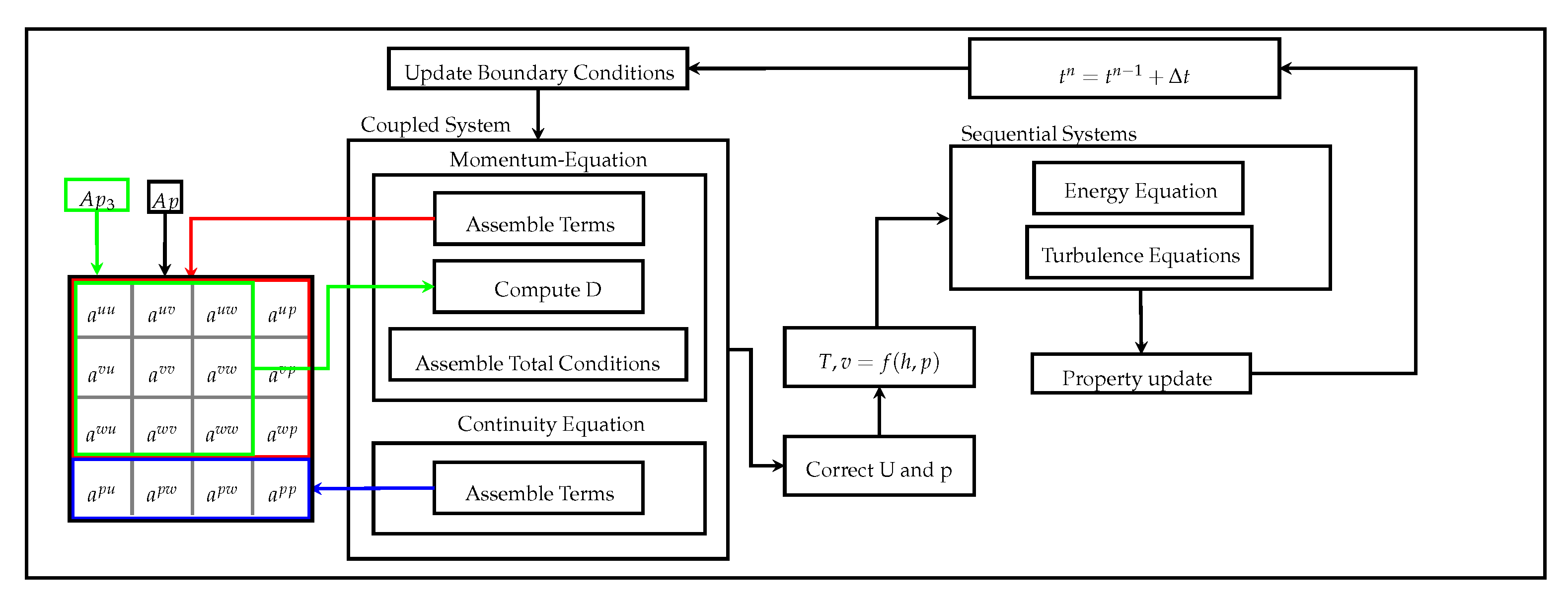
Figure 3 highlights the main body of the coupled solution strategy. The blocks of the flow chart will also define the structure of the present article. In
Section 5, the conservation equations are revisited with a focus on the difference when integrating real gas thermophysics. This is followed by a detailed analysis of boundary conditions mainly focusing on the implementation of total conditions, see
Section 6. The theoretical part is finalized showing the chosen strategies for the update of flow properties in
Section 7.
4. Governing Equations
The above described numerical framework solves the RANS equations as:
in the momentum and energy equation is the deviatoric stress tensor given as:
in the energy equation accounts for diffusive heat flux modeled through Fourier’s approach as:
5. Numerical Discretization of Governing Equations
The governing equations for compressible fluid dynamic analysis are the momentum, continuity, energy and turbulence equations. As described in Equation (
13) the momentum and continuity equations are solved simultaneously to retain the pressure-velocity coupling, followed by a sequential solution of the energy and turbulence equations. A complete derivation of the governing equations, schemes and used solvers would go beyond the scope of this article. Implementation details of the numerical framework is best described in [
9,
10,
11,
27,
28,
29,
30,
31,
32]. The main focus will be the integration of a generalized approach for real gas physics. Partial recapitulation of the derivations concerning conservation equations and boundary conditions will be given where necessary.
5.1. Momentum Equation
The momentum equation remains unchanged compared to the derivation for perfect gas. It is, however, important in order to introduce the coupled solver framework and therefore given in Equation (
19).
accounts for body forces and
is the normal vector of the face with the length of its area. The implicit contributions of the single terms of the momentum equation to the coupled, block-structured coefficient matrix are assembled in what is marked as a red box in
Figure 3. The coupling of the momentum equation to the pressure based continuity equation is dominated by the pressure gradient and assembled in
and
, shown in red in Equation (
13). This is one of the major advantages of coupled solution strategies. The pressure gradient is treated implicitly and thus updated during inner iterations. Segregated solution strategies consider the pressure gradient in the momentum equation as a constant contribution to the source when solving the momentum equations.
5.2. Continuity Equation
For pressure based numerical frameworks, the continuity equation is used to obtain an equation for the pressure which serves as a constraint to fulfill the conservation of mass. Equation (
20) shows the continuity equation in its semi discrete form with
being the velocity flux across a face.
The temporal derivative is expanded using the general assumption that the density can be expressed as a function of pressure and enthalpy. This is a procedure that has been described in [
7]. The linearization of this term is therefore given as shown in Equation (
21). Expressions have to be found for the thermophysical derivatives based on the chosen real gas state equation. This derivation will be exemplified in a later section.
Equation (
21) differs from perfect gas computations where it is usually assumed that the change of density with respect to time can be simply expressed as given in Equation (
22).
The second term of the continuity equation, the convective contribution, is discretized using Newton linearization, see Equation (
23). Variables indexed with ∗ are previous iteration values while variables without this index represent current iteration values.
To avoid checkerboarding pressure fields on collocated arrangements and to introduce the necessary implicit dependency on pressure together with a coupling of the continuity equation to the velocity, the velocity flux of the new time step (
) is computed using the Rhie–Chow [
33] interpolation technique.
is the velocity flux on the face, computed using adjacent cell values through linear interpolation, contributing to the coefficients
and
in the coefficient matrix
. This couples the continuity equation to the velocity field, shown in green in
Figure 3. The pressure gradient
A is evaluated directly on the face, while term
B is evaluated based on cell center values and then interpolated on the face. The term
is the inverted 3 × 3 coefficient sub-matrix
(given in green in
Figure 3) after cell-to-face interpolation.
The density
in Equation (
23) is computed using a first order linearization, to obtain the necessary implicit dependency on pressure. This is in contrast to the derivation for ideal gas, where density is substituted with pressure by simply using the state equation.
Inserting Equations (
24) and (
25) in Equation (
23) and using Equation (
21) in Equation (
20) leads to the final continuity equation in pressure form shown in Equation (
26).
The term introduces an implicit coupling of the continuity equation to the velocity and will therefore contribute to and . Three terms are implicit contributions to , namely , and .
To summarize, the difference in the derivation of the pressure equation for real gas compared to idealized gas is listed below:
Linearization of transient term
Linearization of the density of the actual time step
Partial derivatives and
Thermophysical Partial Derivatives in the Continuity Equation
The derivation of the partial derivatives given above is crucial for the stability of the solver. In this section the derivation of
is given as an example. Expansion of the expression is first done through triple product rule.
Part B1 can extended as follows
In this derivation
is the thermal expansion coefficient and
is the compressibility as given in Equations (
33) and (
34).
Part B2 can be extended as follows
The final expression can therefore be written as given in Equation (
39)
5.3. Energy Equation
The definition of the conservation equation for total internal energy is given in Equation (
40).
For compressible flows it is, however, more convenient to express the energy equation in terms of total enthalpy as
. Equation (
40) is therefore rewritten as Equation (
41).
Compared to ideal gas state equations, the elementary changes are in the modeling of the heat flux. Using Fourier’s law to relate the heat flux to the local temperature gradient with
being the conductivity of the working fluid, Equation (
42). is derived.
This term would lead to a completely explicit contribution to the source of the energy equation, diminishing the stability of the iterative solution procedure. What is needed is an algebraic relation for the dependency of temperature in terms of enthalpy to obtain an implicit formulation of the heat conduction. For calorically perfect ideal gases, this poses no challenge, since enthalpy can be expressed as
. A generalized approach, as considered in this publication, allows no such simplification. To recover at least partly the implicit contribution a first order linearization of the enthalpy is introduced as given in Equation (
43).
Expression
A can be found in
Appendix B and is simply the definition of the specific heat capacity
.
B is zero because the pressure is kept constant during the solution of the energy equation. An expression for the temperature of the actual time step can therefore be found as given in Equation (
45)
Substituting the temperature
T in Equation (
42) using Equation (
45) allows to rewrite the Laplacian contribution as given in Equation (
46). Term
a introduces the implicit contribution providing the needed stability of the discretization.
At convergence term a and b vanish due to their dependency on the correction of enthalpy, hence the heat conduction is modeled accurately. Part b can usually be neglected since the gradient of the heat capacity is often rather small.
6. Boundary Conditions
Considering the implementation of boundary conditions for a coupled framework, it is crucial to identify any coupling between velocity and pressure as well as implicit dependencies on the variable that is solved for. A detailed derivation of the implemented boundary conditions can be found in [
32,
34]. While these articles give a detailed insight in the numerical discretization of a variety of boundary conditions, they assume perfect gas state equations. The focus of this section will therefore remain on the difference when integrating real gas state equations.
6.1. Total Conditions
The use of total conditions at the inlet is a very common boundary condition. A detailed derivation is therefore given in what follows. As already shown, in a coupled framework, the momentum and continuity equation are assembled into one system of equations. In order to properly account for the boundary contribution, each term of the conservation equations has to be analyzed with respect to the constraint given by the user. This is described in detail in [
32] for ideal gas.
The derivation of total conditions in this section is given by first providing the algorithm for consistent total to static conversion. The algorithm uses the common assumption of an isentropic deceleration to stagnation conditions but without all the simplifications valid only for perfect gas. This is followed by the discretization of the Navier–Stokes equations itself. With the exception of the pressure gradient term, this is in close agreement to what is given in [
32]. The main body of this section will therefore be a detailed revision of the discretization of the pressure gradient term when dealing with real gas state equations.
6.1.1. Isentropic Total-to-Static Conversion
As already mentioned above, the computation of static values using given total conditions can no longer be obtained using well-known algebraic relations. It is, however, possible to find an iterative solution procedure to accurately compute these quantities. The algorithm used is a Newton–Raphson root finding method. The roots are the two underlying constraints of the total to static conversion. Root 1 as given in Equation (
47) is the isentropic constraint, while root 2 as given in Equation (
48) is simply using the definition of total enthalpy.
In the following the Newton–Raphson root finding method is explained as a reference. This procedure is later applied to a variety of solution strategies used for finding iterative solutions for thermophysical changes in real gas. The procedure starts with a first order Taylor expansion of the roots.
From Equations (
47) and (
48) it is known that these equations are equal to zero. Hence we can reformulate them as shown in Equations (
51) and (
52).
The corrections
and
are defined as:
This is system of equation is then rewritten in matrix form as:
By inverting matrix
A the system can be solved as shown in Equation (
56)
The variables
are then updated with the correction and the procedure repeated until certain convergence criterion is achieved. Applied to the roots given in Equations (
47) and (
48) with
and
, the following derivatives have to be found using the chosen real gas state equation.
can be found in
Appendix B.
is equal to
and
can be replaced with
by using Maxwell relations.
is found as given in Equation (
59).
In a second step,
is derived from Equation (
6) as given in Equation (
60).
Hence Equation (
59) can be written as given in Equation (
61). The derivatives of the pressure are easily found through the chosen state equation.
6.1.2. Pressure Gradient Term
As already pointed out, the discretization of the Navier–Stokes equation for given total conditions is best described following what is written in [
32]. When integrating real gas state equations, the only difference is in the discretization of the pressure gradient term of the momentum equation. Using Green–Gauss theorem to rewrite the volume integral value of the pressure gradient as a surface integral, this term is written as given in Equation (
62). An expression for the value of the pressure at the boundary face is therefore needed. The requirement is a strong coupling to face adjacent cell values of pressure and velocity, leading to an implicit contribution to the coefficient matrix. This ensures a robust integration of boundary conditions into the linearized equation system.
Using the well known strong coupling between pressure and velocity, a first order linearization of the pressure with respect to the velocity flux
is introduced as given in Equation (
63).
b indexes values evaluated at boundary faces. Again, the velocity flux is defined as
with
being a face normal vector with the length of the area of the face. As for the continuity equation this leads to an implicit contribution to the cell velocity and an implicit coupling to the pressure field of the continuity equation.
What is needed is an expression for the gradient
and the value of the velocity flux of the new time step
. The value for the velocity flux is computed using Rhie–Chow interpolation, given in Equation (
64).
The gradient of the pressure at the boundary is approximated as given in Equation (
65).
With
being the cell pressure value and
the normal distance from face to cell center. Inserting Equation (
63) in Equation (
64) leads to the final definition for the boundary pressure value given in Equation (
66).
The only unknown is therefore the gradient of pressure with respect to the velocity flux
. This is usually computed using the algebraic relations for the static to stagnation conversion, given in Equation (
70) for incompressible cases and Equation (
71) for compressible cases.
As explained before, direct algebraic relations that describe the change in pressure of a fluid particle when brought to rest isentropically are not explicitly available for the general case of a real gas. To approximate the gradient
the definition given in Equation (
72) is used.
The static value of the pressure is computed using an iterative scheme given the total conditions based on
and
as described above. In a second step, the velocity is computed that corresponds to a slightly increased pressure level
, following an isentropic change. Hence the roots are:
In addition to the derivatives given in the section dealing with total to static conversion the partial derivatives of the pressure are needed.
Using the values for
and
the value of the static enthalpy
is computed according to Equation (
76). The calculation of internal energy follows the previously explained integration along paths.
The velocity magnitude corresponding to these updated values is further found through the definition of total enthalpy as given in Equation (
77).
The value for the derivative of pressure with respect to velocity is then found by substituting these results into Equation (
72).
7. Update of Flow Properties
As shown in
Figure 3, the outcome of the conservation equations for momentum, continuity and energy are updated values for velocity, pressure and total enthalpy. There are, however, many other flow properties that are not directly obtained but which have to be computed based on these known values. This may be because they are intrinsically necessary for the solution procedure, as, e.g., density or viscosity, or because they are valuable quantities for post-processing such as Mach-number or entropy. This section explains their computation when operating in regions, where real gas effects can no longer be neglected.
7.1. Update of Temperature and Density
Given the velocity, the pressure and total enthalpy from the conservation equations, it is possible to update the temperature and density independent of the state equation. First, the static enthalpy is computed using the given total enthalpy
and the velocity based on the solution of the RANS equations.
The value for temperature and density are computed using the Newton–Raphson method. The roots of the method are:
The rest of the Newton–Raphson root finding procedure can be done in analogy to
Section 6.1.1.
7.2. Total Pressure and Total Temperature
In contrast to the problem of specified total conditions for boundary conditions as described in
Section 6.1, finding stagnation values for static conditions is usually required for the remaining cells and boundary faces of the computational domain. As described, no explicit relation exists for the static to stagnation conversion, asking for an iterative procedure for the isentropic state change. Consequently, Newton–Raphson root finding method is used. Given the static values of temperature and specific volume, the two roots therefore are given in Equations (
81) and (
82). With
and
being the requested stagnation values
and
.
As written above, having the roots of the Newton–Raphson method defined, the solution is in close analogy to what is given in
Section 6.1.1. With the stagnation values for
and
the total pressure is easily reconstructed using the chosen state equation.
8. Validation and Results
This section provides an assessment of the generality and accuracy of the implemented numerical solution procedure when dealing with real gas state equations. Initially, the well-known transonic bump of Peric [
35] is used. This test case is used to test the consistency of the implemented procedures when perfect gas state equations are used. The expressions and iterative algorithms given above have to return the same solutions as when using the mentioned algebraic relations only valid for perfect gas. Validity of the implemented procedures is given through comparison of the RMS-residuals.
The second test case is a transonic nozzle configuration operated using steam based on the IAPWS-97 formulation [
13]. Results are compared to a commercial code.
To demonstrate the generality of the approach to any type of state equations, cubic state equations are used for a two-stage radial compressor. Results are compared against commercial code and measurement data.
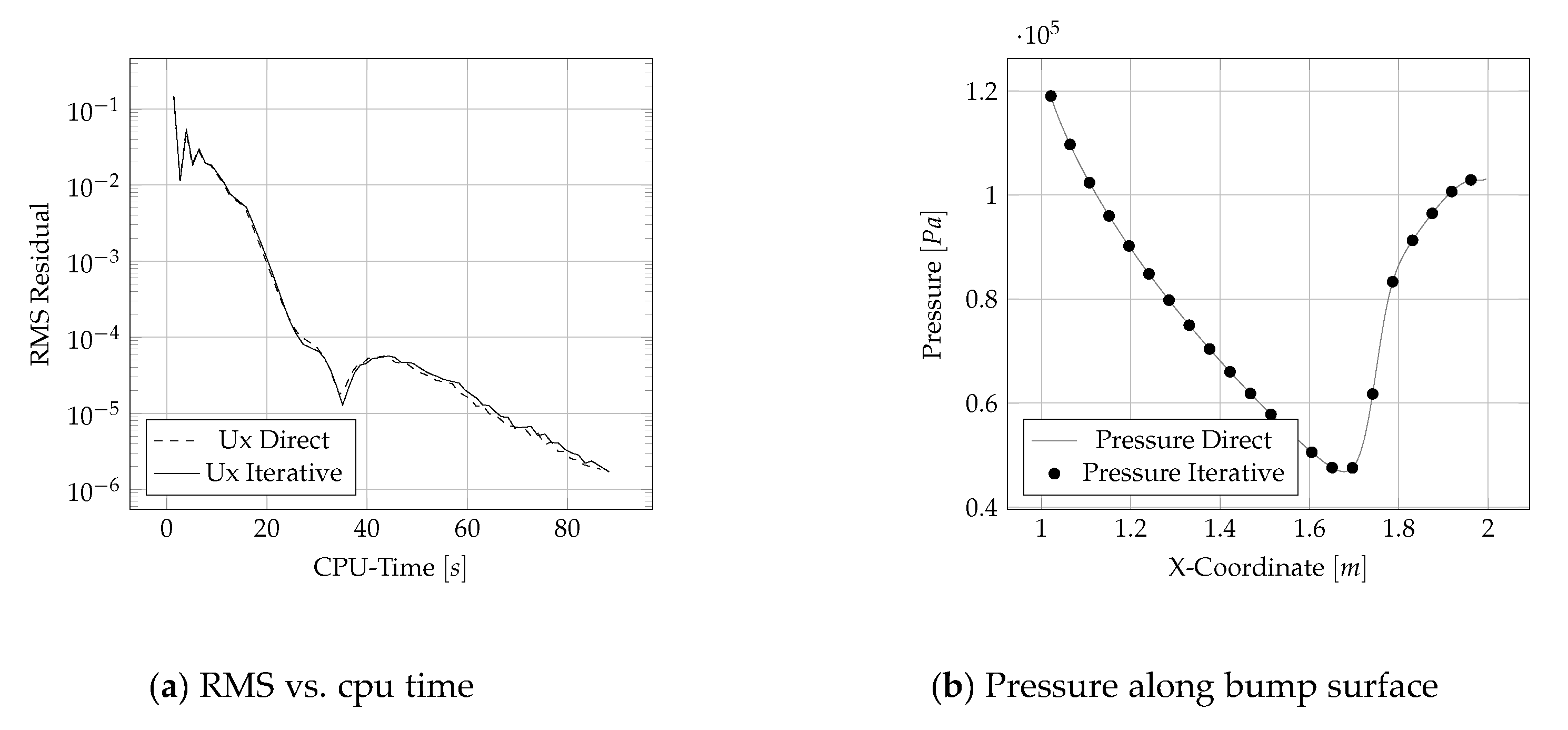
8.1. Consistency of the algorithms for Perfect Gas State Equation
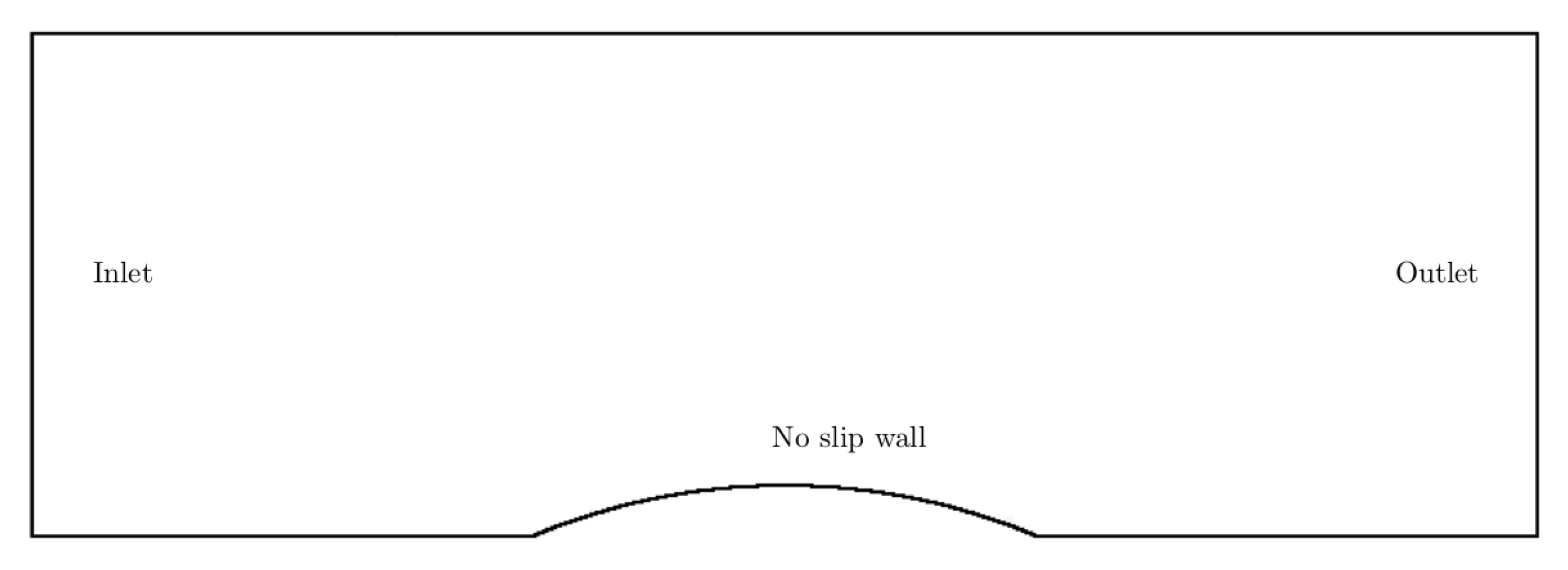
The transonic bump test case of Peric [
35] is given in
Figure 4. The thickness to chord ratio of the bump is 10% and the computational domain consists of 53,000 quadrilateral grid elements. The inlet boundary conditions is set to a total pressure of 1.4 bar and a total temperature of 783K, turbulence intensity is 0.1% and the eddy viscosity ratio is set 2. The outlet static pressure is 1bar. The working fluid is air with the turbulence modeled using the
k-
-SST model of [
36].
To prove the consistency of the implemented generalized approach, the results should reduce to the same output as when directly using perfect gas assumptions, when deriving the fundamental equations.
Figure 5a shows the comparison between the direct solution and the iterative procedure for the ideal gas case. The small difference results from the fact that the generalized approach uses an iterative procedure to evaluate isentropic conditions and to update temperature and density, hence the accuracy of the solution is limited by the convergence criterion. For reference the pressure distribution along the bump surface is given in
Figure 5. The solutions coincide for the two methods.
8.2. Validation Using IAPWS-97 Real Gas State Equations
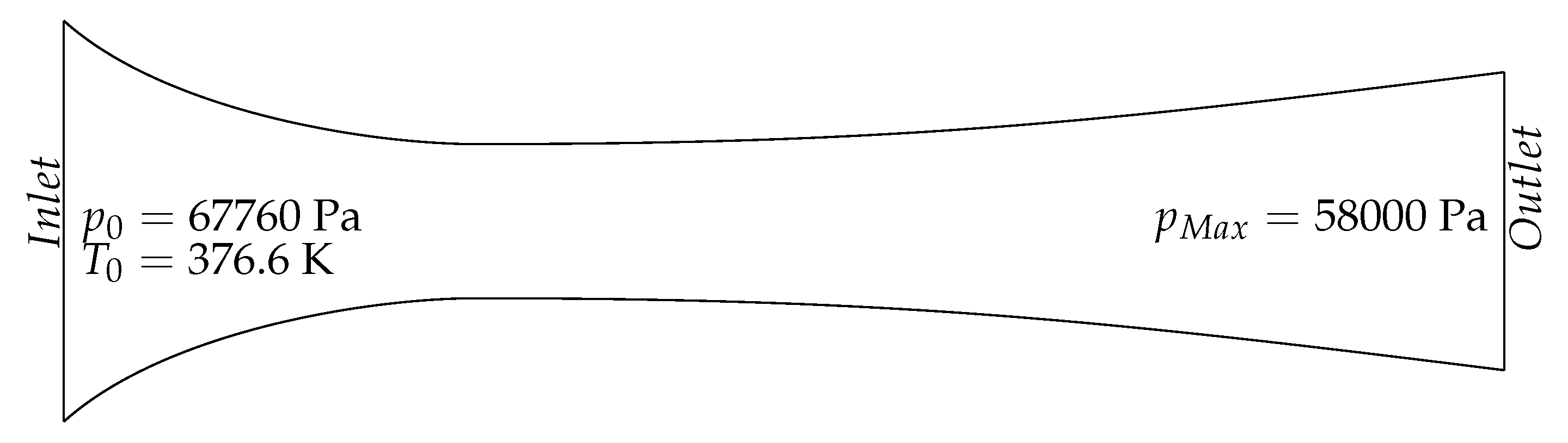
The second test case is a nozzle configuration published by Moses and Stein [
37]. This configuration is frequently used to investigate droplet growth and real gas flow physics, see e.g., [
38]. Since this investigation of real gas flow physics lays the basis for further extension to multiphase flows, this test case provides an ideal reference for testing the robustness of the implementation.
Figure 6 shows the overall domain.
The inlet total pressure was set to 67,760 Pa, while the outlet static pressure was varied. From an outlet pressure of 58,000 Pa the pressure was constantly lowered until choking flow configurations were obtained. As for the transonic bump test case before, the
k-
SST turbulence model of [
36] was used.
Initially, the computational domain is thermophysically assigned to region 2 of the IAPWS standard, i.e., gaseous state. When lowering the outlet static pressure, the temperature drop due to the acceleration in the nozzle theoretically leads to cells that are assigned to the two-phase region of the IAPWS standard, i.e., region 4. However, it was observed that the commercial code software restricts to region 2 of the IAPWS standard, when running single fluid.
Figure 7a shows the centerline temperature along the nozzle geometry from inlet to outlet and demonstrates this behaviour.
The dashed line is the solution of the in-house code, the continuous line shows the solution of the commercial code. Extrapolation of region 2 into the two-phase region 4, as done by the commercial code, leads to considerably lower temperatures in the throat area. The in-house code applies the proper formulations of the IAPWS standard if phase transition is detected. However, it needs to be mentioned that both solutions do not entirely reflect the full reality. Although the properties of the water are clearly better described using the state equations for the two phase region 4, it is not equal to a full two-phase simulation. The assumption of instant thermal equilibrium for example is an oversimplification of the actual problem and prevents an accurate modeling of the phase change. Being able to switch the state equation in a region where the flow properties change rapidly, however, is a demonstration of the stability of the underlying methods. An option was implemented that allows a restriction of the in-house code to stay within a prescribed region. In case a transition into the two-phase region is detected, the values of region 2 are extrapolated. The effect is presented in
Figure 7b. The solutions obtained with the in-house framework match the commercial code.
The following validation was therefore carried out restricting the framework to region 2 of the IAPWS standard.
Figure 8 shows the temperature and pressure distribution along the symmetry plane for three different outlet pressures. As can be seen the results are in close agreement with commercial code results, over the complete range from subsonic flow (black lines) to transonic flow (gray lines) until supersonic, chocking flow regime (light gray lines). In
Figure 8a a continuous line can be seen for the 15,000 Pa case for both numerical algorithms. The pressure curve in
Figure 8b does not show this sharp limit. This is because the value of the pressure in the interior of the domain is a direct outcome of the linearized equation system, while temperature is computed as a post-processing field based on the values of pressure and enthalpy. In this post-processing step the values for the temperature are limited to 273.25 K which is the limit of defined temperatures of the IAPWS-97 formulation.
8.3. Two-Stage Radial Compressor
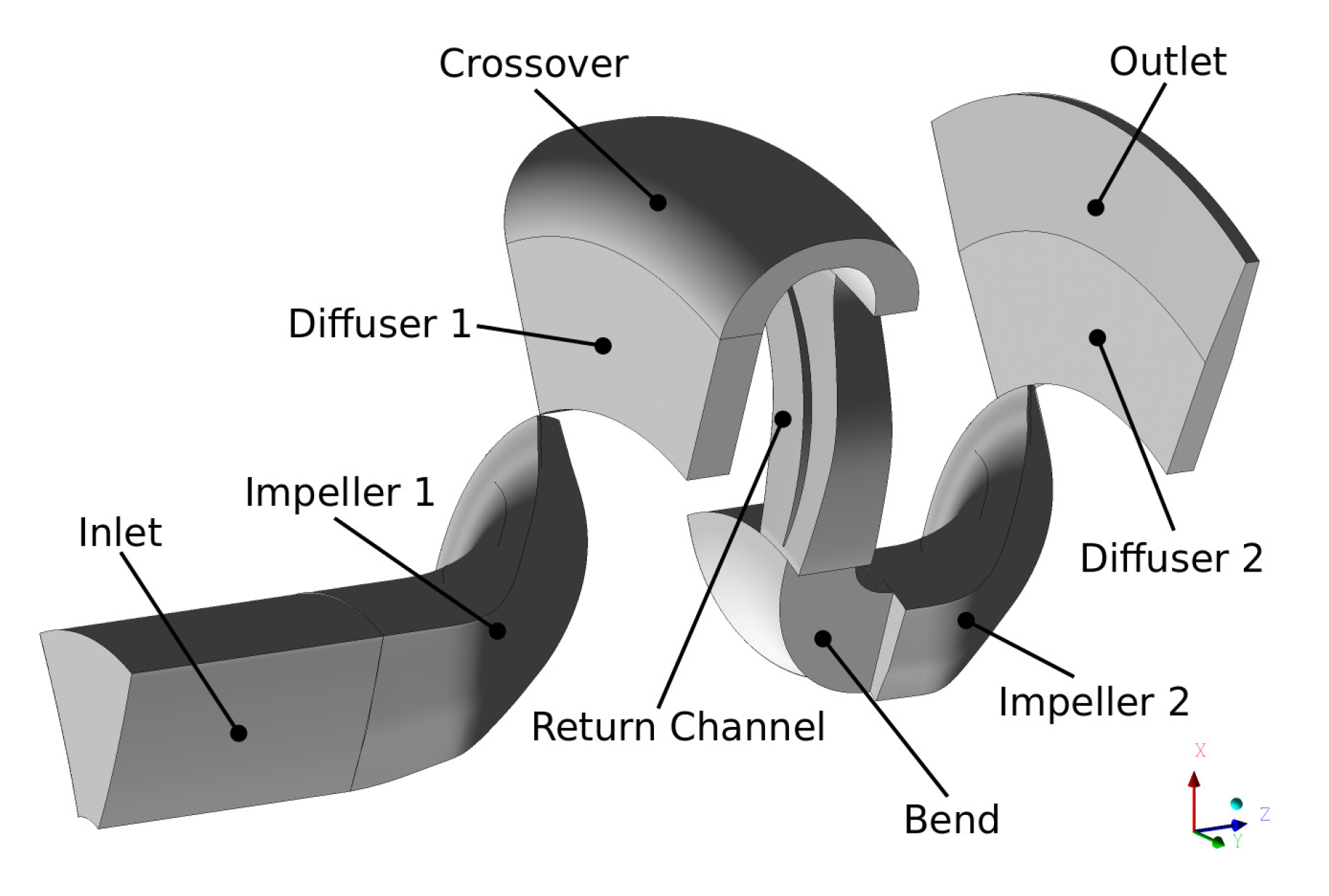
Final validation is carried out on the basis of a two-stage radial compressor with a refrigerant as a working fluid. Due to the governmental requirements on the global warming potential (GWP), a replacement of the refrigerant became necessary. This led to a redesign of the components accompanied with measurements herein used for the validation of the implemented numerical model. The main objective of the measurement campaign was to gain information on the surge line under various operating conditions to allow for a controlled operation of the compressor. A vaneless radial diffuser follows each impeller while the return channel contains a single row of stationary blades to reduce the swirl before the second impeller.
Figure 9 shows the individual parts.
8.3.1. Measurement Setup
The two stage compressor was installed in the laboratory of the Institute for Thermal Energy System and Process Engineering at HSLU in Lucerne. Restriction in the laboratory environment, however, led to operating conditions, which are not in line with the design. This concerns mainly the inlet temperature and pressure levels, which could not be tuned to design conditions.
In order to account for this inconsistency, dynamic scaling was applied to match the operating conditions of the design. The rotational speed of the compressor was corrected using Equation (
83), with
f being the design frequency and
the corrected frequency of the laboratory setup. The mass flow is then corrected based on the non-dimensional mass flow as given Equation (
83) for comparison with the design conditions.
8.3.2. Numerical Setup
The manufacturers choice for the real gas state equations was the standard Peng–Robinson model as given in Equation (
2). In order to account for the temperature dependency of the dynamic viscosity, the interacting sphere model given in [
39,
40] was applied. Furthermore, the thermal conductivity is modeled using the modified Eucken formulation as described in [
41]. This decision is mainly based on comparability considerations concerning the CFD computations which have been carried out using a commercial tool during the measurement campaign. Of the available models in the commercial tool, the Peng–Robinson EOS showed the smallest error for the chosen working fluid and operating conditions.
Table 1 shows the relative error comparing the chosen thermophysical models against tabulated values from REFPROP [
42] over the operating range of the working fluid. A significant error can be seen in laminar conductivity and viscosity; however, this effect is negligible since dominated by the turbulent contributions. The error in the heat capacity was tested on its effect on the results and a change in the value in the range given in the table did not have a significant influence on the final results.
The ideal gas contribution of any internal energy change (Path B in
Figure 2) is evaluated using a fourth order polynomial for the specific heat capacity at constant pressure. Turbulence is accounted for by the use of the Menter-SST model [
36] with automatic wall treatment. The mesh consists of a total of nine different regions connected with fourteen interfaces for general grid connections and six in-house developed mixing planes, connecting the regions with different periodicities. Details on the implementation of the mixing plane can be found in [
43]. The computational domain consists of 4 mio cells with
values around 20.
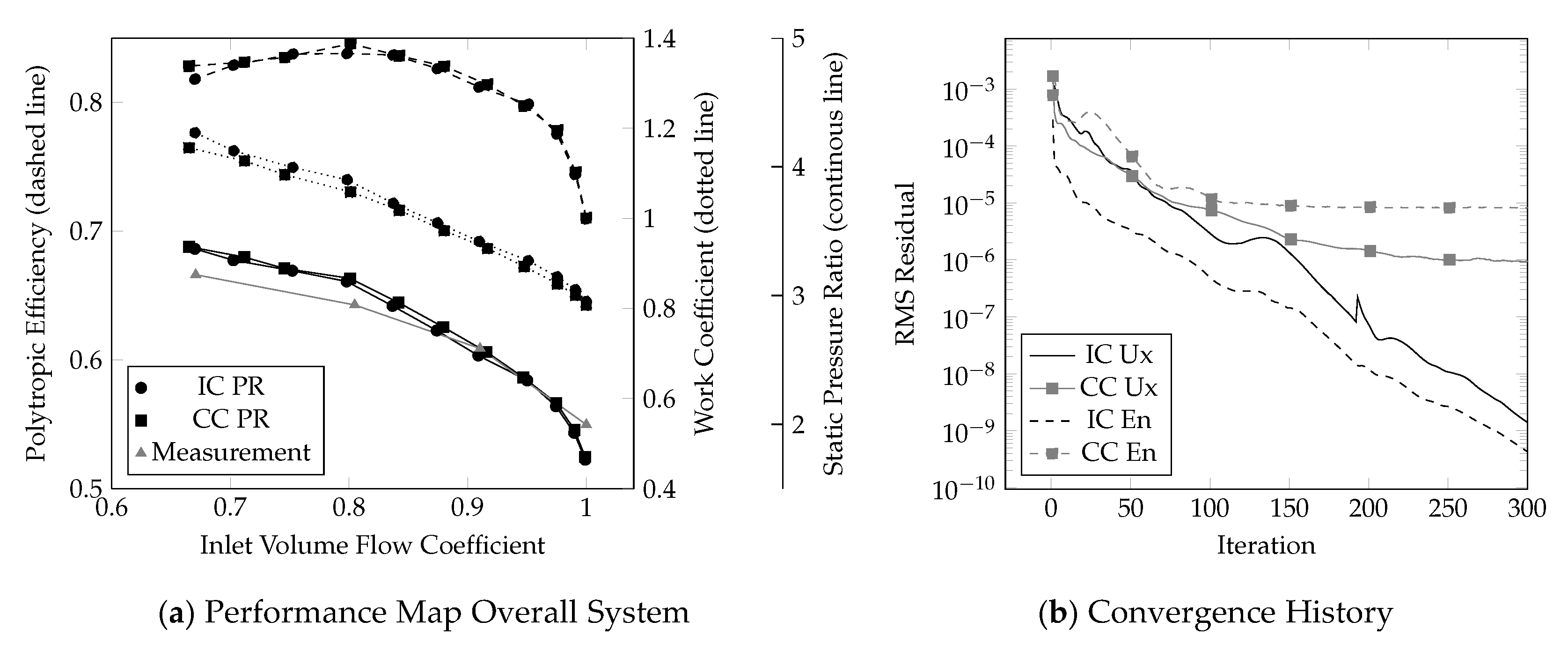
8.3.3. Global Performance Comparison
The complete operating range for a given rotational speed was computed using the above described real gas models by continuously increasing the backpressure until the stability limit was reached. In order to assess the quality of the results, the solutions are compared against commercial code results and measurement data. At the time, the only measurement data available for comparison was the pressure ratio. This is due to the fact that the main objective of the measurement campaign was to find the surge lines to allow for a controlled operation. To validate the implemented procedure, the results are further compared with commercial code results by plotting polytropic efficiency Equation (
84) and work coefficient Equation (
85) against flow coefficient Equation (
86). The circumferential velocity
is evaluated at the radius (
) of the first compressor outlet.
Figure 10a shows the results for the whole operating range from choking flow to the stability limit. The legend entries IC and CC stand for the in-house code and commercial code, respectively. It is evident that the solutions are in very close agreement, indicating the consistency of the underlying thermophysical models. Comparison against measurement data was only available in terms of static pressure ratio, shown in gray. The differences in the results between numerical predictions and measurement setup are dominated by the limitations of the laboratory setup as explained in the section covering the measurement setup.
In order to provide a reliable tool for the design of turbomachinery applications operating in real gas thermophysical regions, accurate numerical solutions are not enough. To allow for a high work efficiency and reduced resources, numerical stability of the iterative process together with a small computational overhead are equally important. Investigations considering the convergence behavior have shown promising results as can be seen from
Figure 10b.
In order to examine the effects of real gas modeling compared to perfect gas thermophysical models, cpu time was compared as well. An increase of about 50% compared when switching to real gas models could be observed for this test case setup. A value well within what is observed from commercial code results.
8.3.4. Real Gas Effects
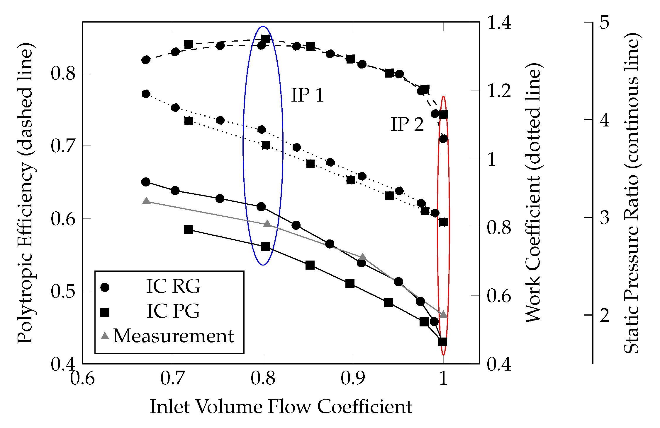
In this section, we only compare solutions obtained with the in-house framework. The investigation focuses on differences in the results when using real gas models instead of perfect gas assumptions. In order to do so, the characteristic was recomputed using standard models for perfect gas as Newtonian viscosity, constant heat capacity and Prandtl’s law for the conductivity based on average values from the real gas solutions. The results are shown in
Figure 11. Lines with square markers correspond to solutions of the perfect gas model (PG) and lines with circular markers correspond to the real gas solution (RG) based on Peng–Robinson state equation as already shown in
Figure 10a.
With respect to polytropic efficiency (dashed line), similar results are obtained for flow coefficients above the peak efficiency point. Considering peak efficiency, a difference of ∼2% can be found. While this is surely not negligible, the differences are too small to draw any general conclusions. Comparing the curves of static pressure ratio (continuous line), it is however clear that when using perfect gas state equation lower back pressure is necessary for the same volume flow coefficient. Using the perfect gas model, it was not possible to reach the same pressure levels as when using the real gas model. The compressor stability limit was detected at much smaller levels of back pressure and the flow coefficient dropped much faster for the perfect gas when increasing the back pressure.
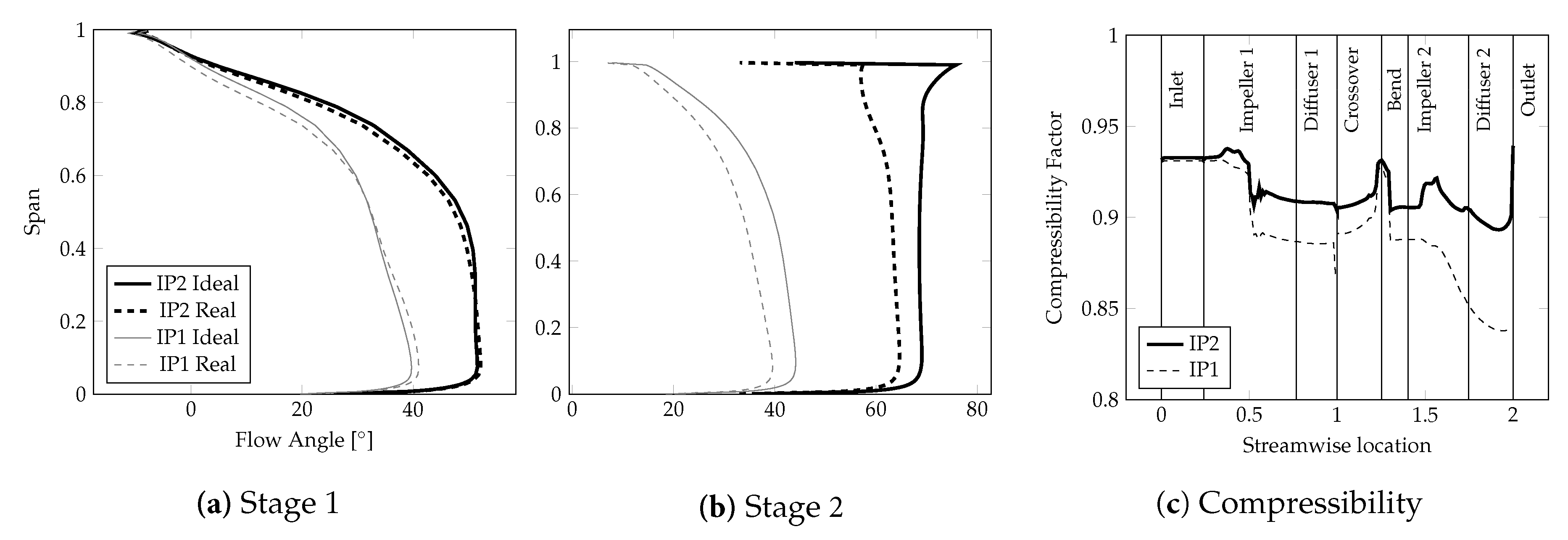
Further investigation of the marked regions (IP1 in blue, IP2 in red) show the differences. IP1 corresponds to peak efficiency for both setups, IP2 are choking conditions. The operating points of the CFD simulation were set by fixing the value of the pressure at the outlet. As can be seen from IP1 (peak efficiency), to obtain the same flow coefficient, the perfect gas model needs a much smaller static pressure ratio between inlet and outlet. In fact, the outlet pressure of the perfect gas simulation is roughly 13% lower than for real gas. This is in contrast to IP2 (choking conditions) where pressure ratio and flow coefficient are in close agreement. This can, however, be explained by
Figure 12c. Under choking conditions, the flow is much closer to ideal gas behavior (Compressibility z = 1), thus the effect of real gas modeling is smaller.
Comparing the exit flow angles from
Figure 12a the general orientation between real gas and perfect gas in stage 1 do not show a significant difference. This is independent whether choking or peak efficiency is considered. Increasing deviation can be found when comparing the results in stage 2, see
Figure 12b. An explanation can be found when plotting the average compressibility factor in streamwise direction given in
Figure 12c, showing the increasing deviation from ideal gas state through the compressor. This deviation from perfect gas modeling assumptions become more and more dominant with increasing back pressure (denser gas), explaining the increased difference in polytropic efficiency for the peak efficiency point.
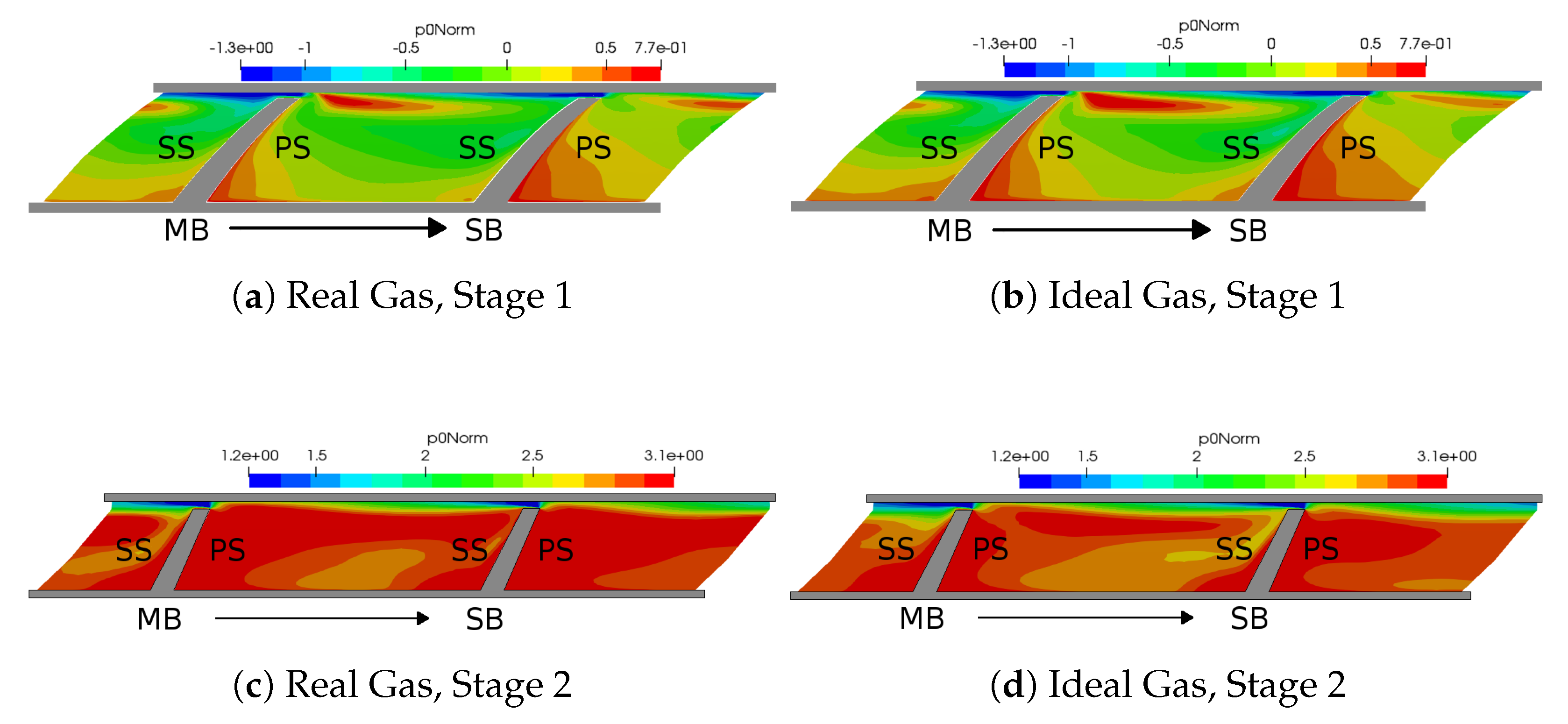
A normalized dynamic pressure was computed in order to compare the dynamic contribution between real and perfect gas computations as given in Equation (
87).
Figure 13 shows the results for IP1 (Peak efficiency) at sections close to the impeller outlets. For stage 1 the results are comparable, differences however become present in the second stage. This is especially true for the suction side (SS) of the splitter blade (SB), where the dynamic contribution is much lower.
These differences in terms of compressor dynamics when switching between real and perfect gas model explain the importance of an accurate representation of the thermophysical properties and derivation of the conservation equations. Using perfect gas models would lead to errors in the design of blade geometries because the flow physics are not captured accurately.
9. Conclusions
The present work summarizes the necessary steps during the derivation and implementation of Navier–Stokes equations into a pressure based numerical framework when operating in non-ideal gs conditions. Detailed analysis is given concerning the discretization of the conservation equations when using real gas state equations. This is extended furthermore to the development of boundary conditions and iterative procedures for the update of various flow quantities. A transonic bump case was chosen to demonstrate the consistency of the modifications. The added iterative solution procedures for the thermophysical states reduce to the same results as the direct algebraic relations for perfect gas.
The real gas models were then tested using two different state equations, once using the IAPWS-97 formulation for water and once using the Peng–Robinson cubic state equation. Comparison against the commercial code results was carried out using the IAPWS-97 formulation on a transonic nozzle configuration. It was found that commercial code extrapolates the gaseous equations into the two-phase region. Applying the same treatment to the in-house code then allowed further comparison and a close agreement between the two frameworks was found.
Cubic state equations were then applied to an industrial type compressor setup and compared against commercial code results and measurement data. It could be proven that the implemented procedure is not only able to accurately replicate commercial code results but also leads to a stability of the iterative scheme that goes beyond the capabilities of the used commercial tool. Comparison against perfect gas assumptions justify the increased complexity of the implementation. It could be demonstrated, based on overall performance prediction and local flow features, that the assumption of perfect gas shows its limitation under certain operating conditions, especially away from choking conditions. At moderate backpressure levels, however, i.e., high volume flow rate, the assumption of perfect gas might be a viable option. Especially during preliminary design phase, the possibility to use perfect gas assumption without great loss of accuracy can lower the computational costs and therefore increase the throughput. For a thorough analysis of the geometry, real gas state equations are, however, a necessity.

 ,
, 


