
Continuous Adjoint-Based Optimization of an Internally Cooled Turbine Blade—Mathematical Development and Application †

 , , , and
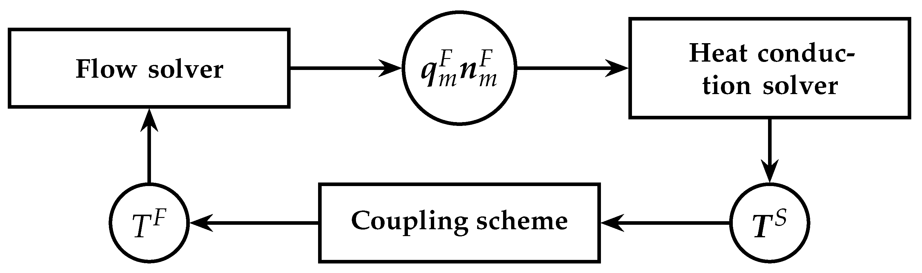
Abstract
:1. Introduction
2. Governing Equations
3. Continuous Adjoint Formulation
3.1. Development of the Integral
3.2. Development of the Integral
3.3. Development of the Integral
3.4. Development of the Integral
3.5. Field Adjoint Equations (FAEs) and Adjoint Boundary Conditions (ABCs)
3.6. Expression for
4. The PUMA Software
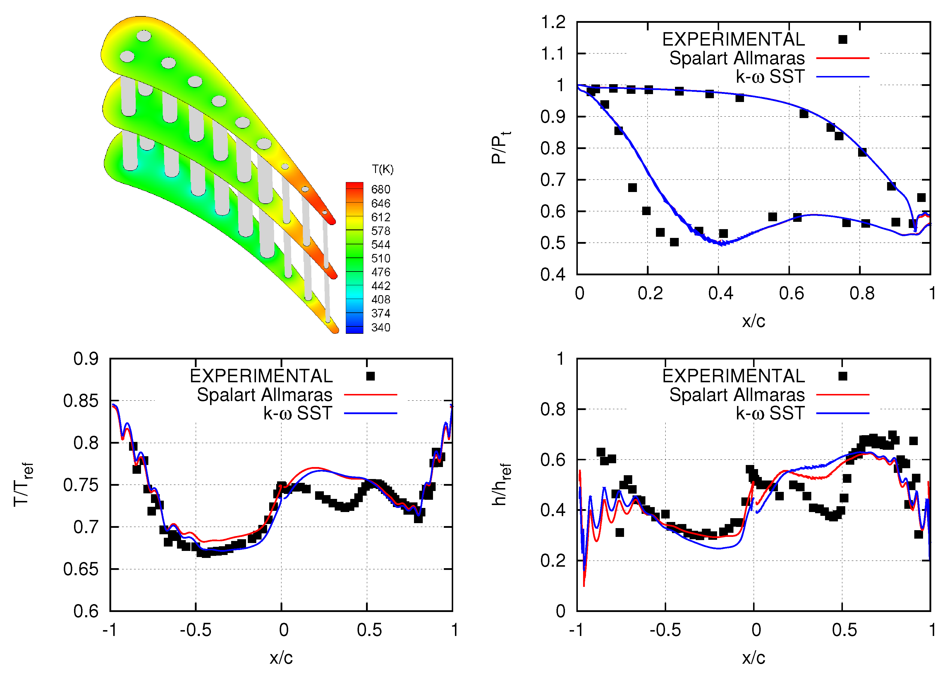
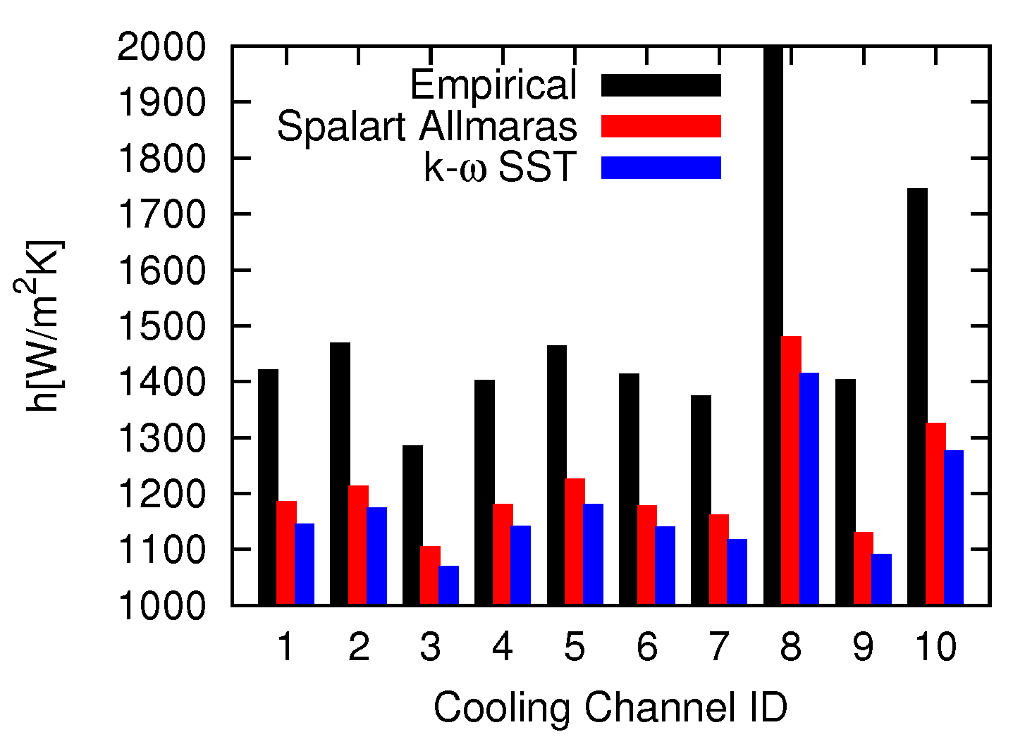
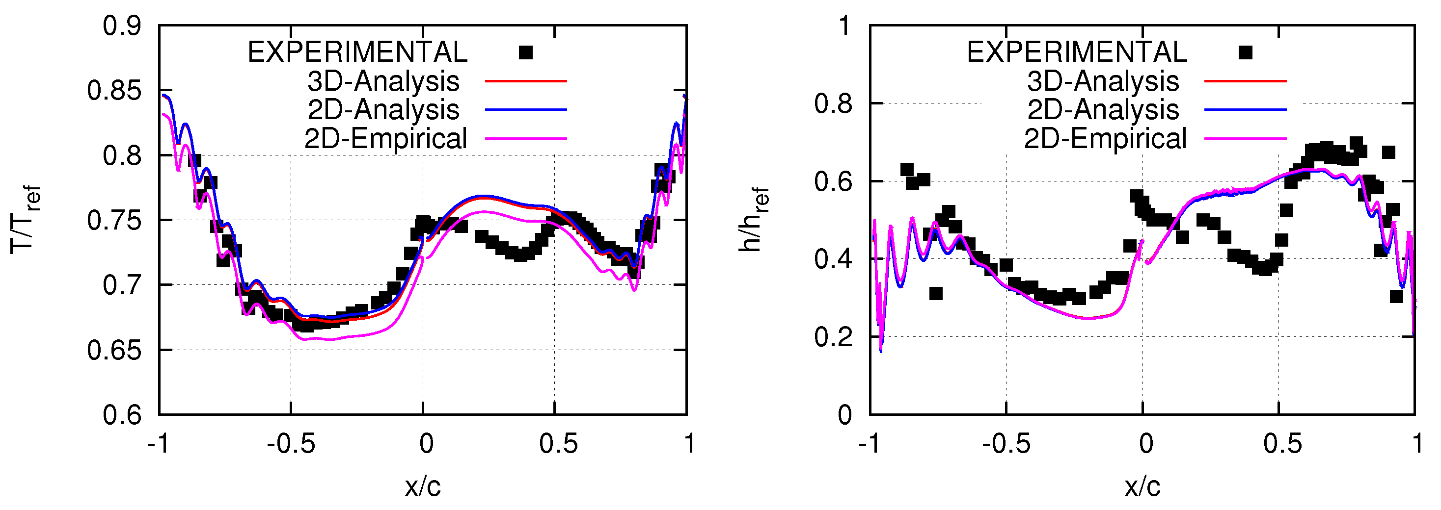
5. CHT Analysis of the C3X Turbine
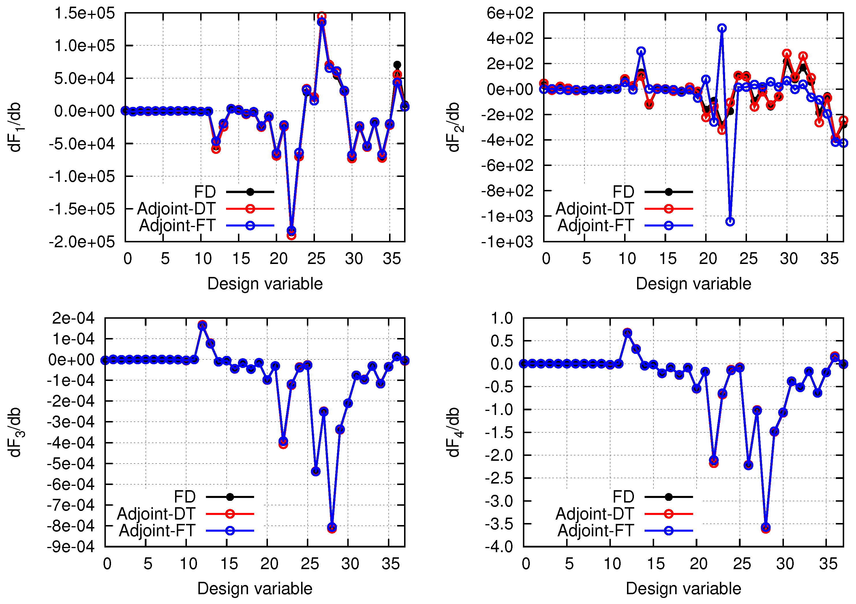
6. Verification of the Adjoint Sensitivities
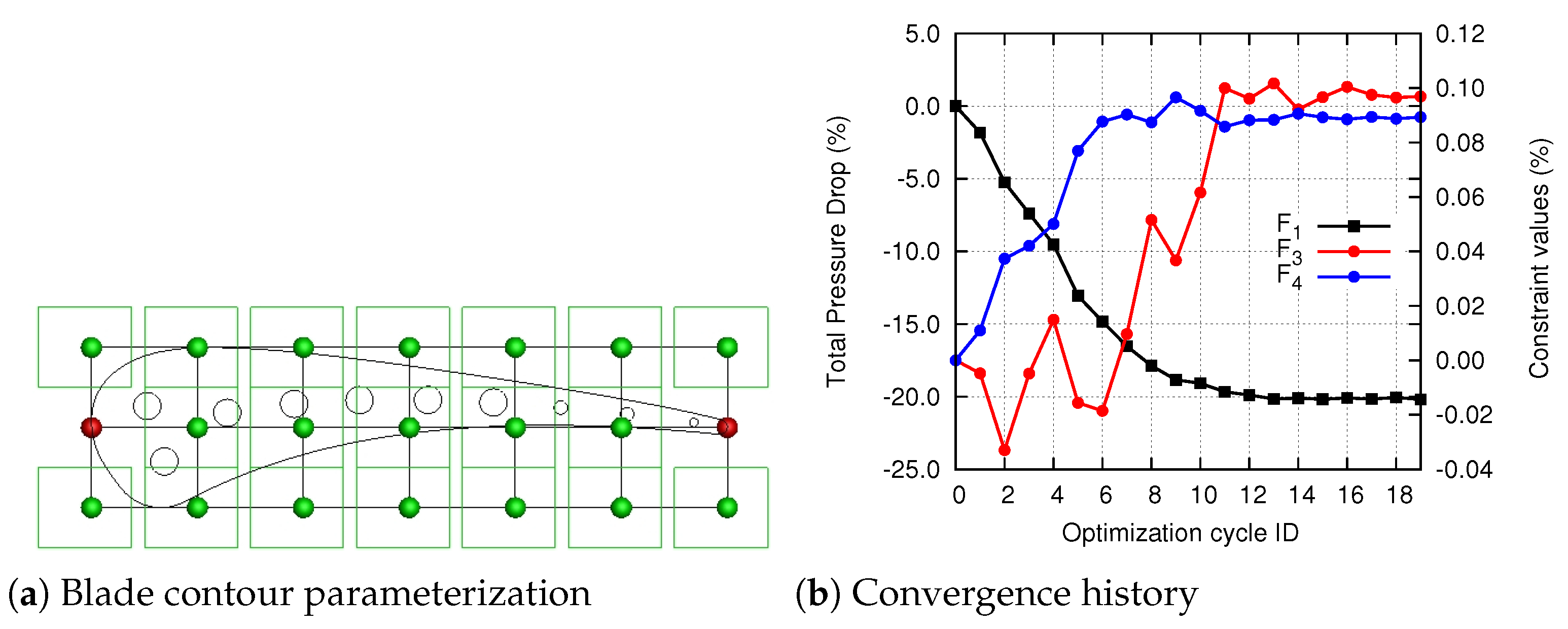
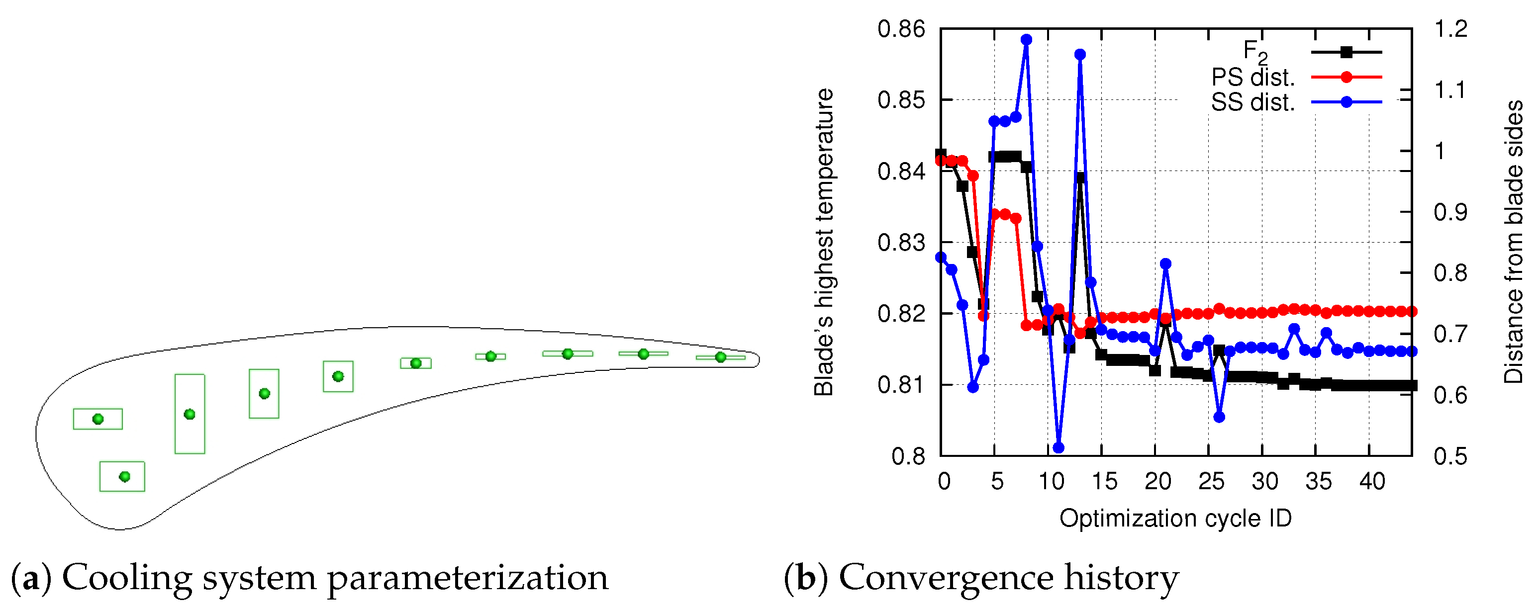
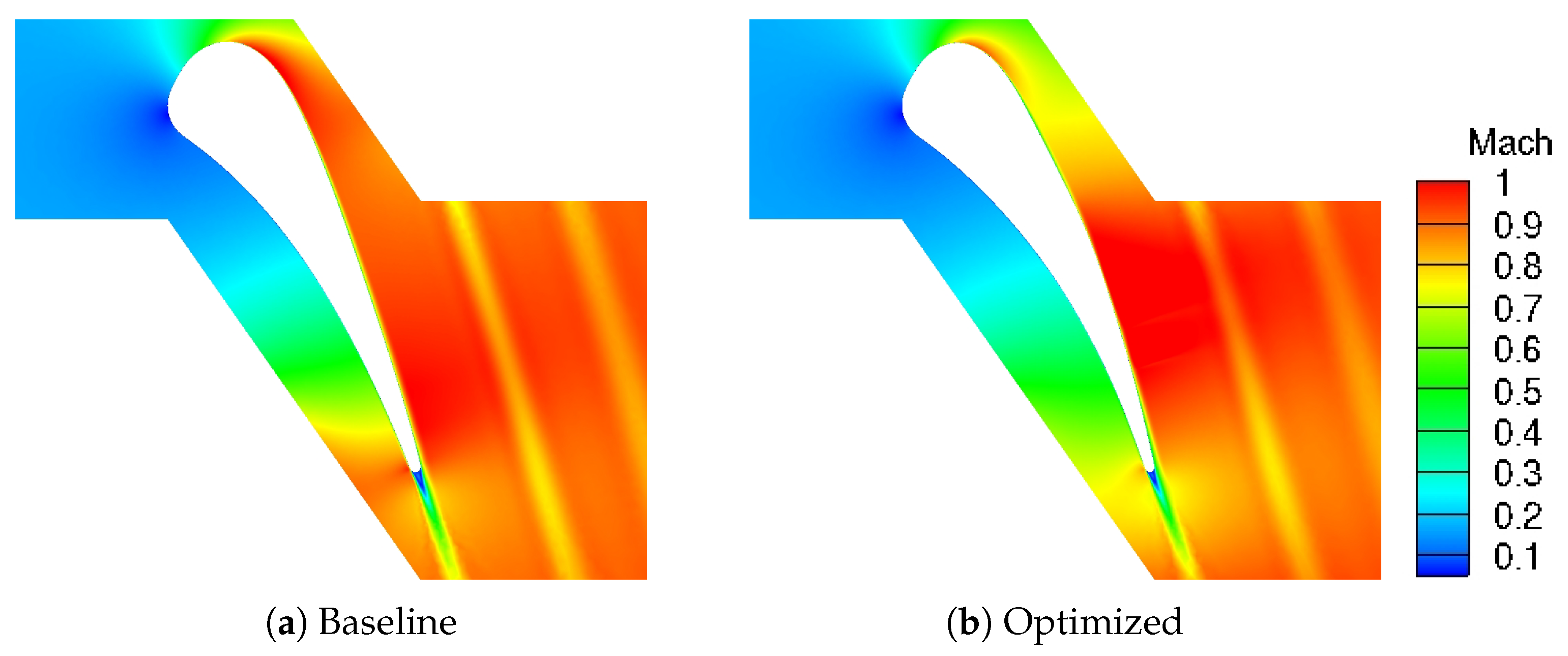
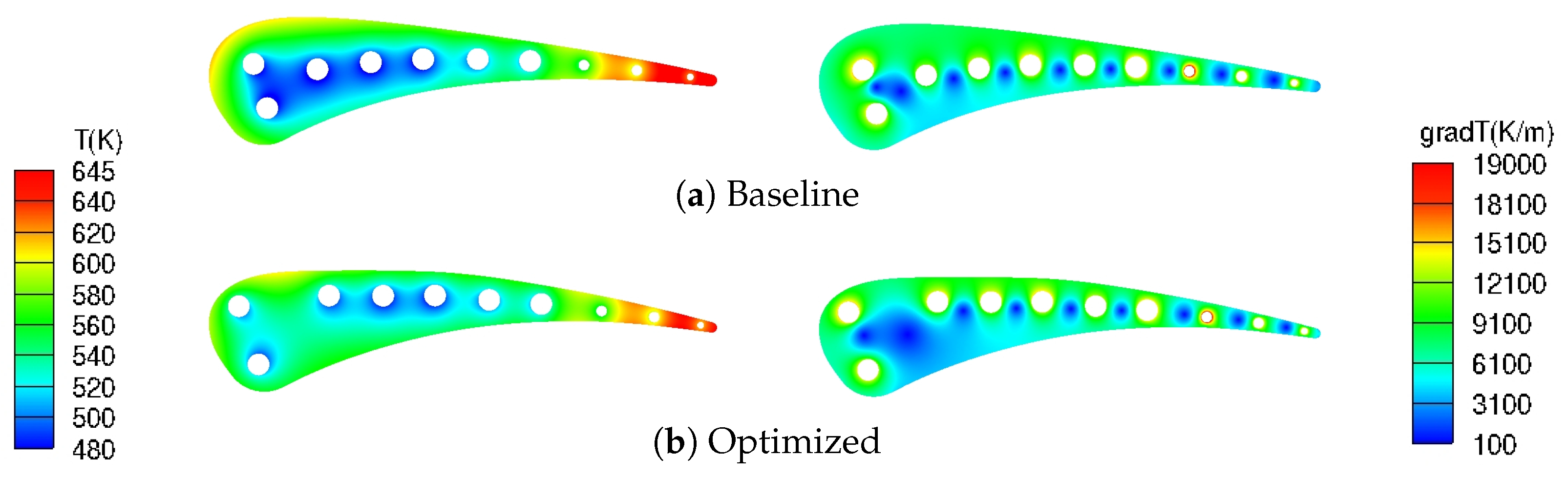
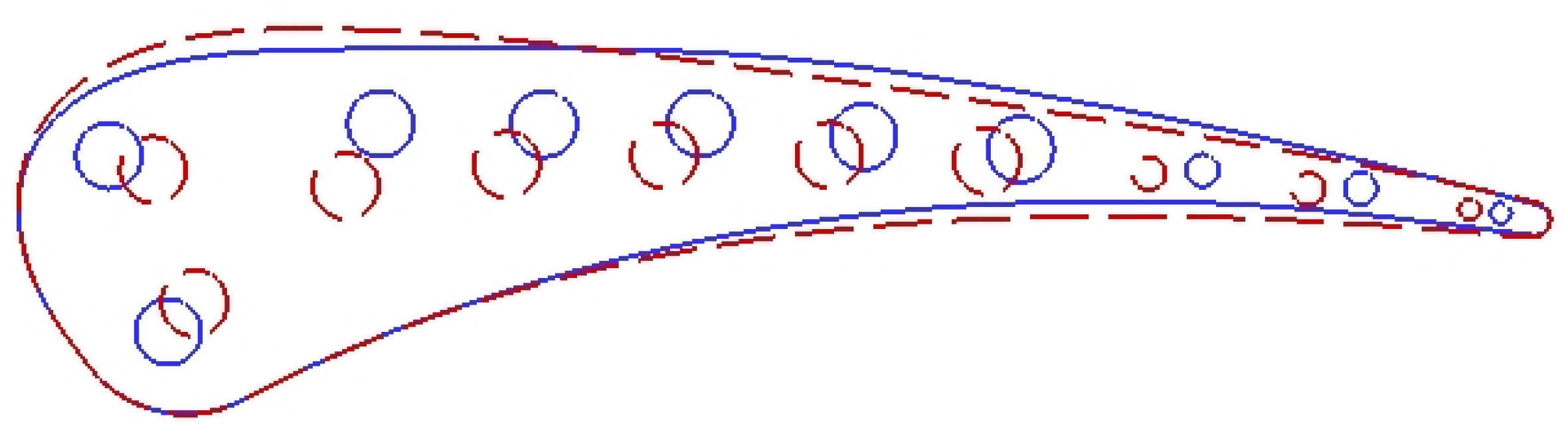
7. CHT Optimization of the C3X Turbine
8. Conclusions
Author Contributions
Funding
Institutional Review Board Statement
Informed Consent Statement
Data Availability Statement
Conflicts of Interest
Abbreviations
| CFD | Computational fluid dynamics |
| CHT | Conjugate heat transfer |
| FAE | Field adjoint equation |
| FDs | Finite differences |
| FSI | Fluid–solid interface |
| GPU | Graphics processing unit |
| NURBS | Non-uniform rational B-splines |
| RANS | Reynolds-averaged Navier–Stokes |
| SD | Sensitivity derivative |
References
- Moretti, R.; Errera, M.; Couaillier, V.; Feyel, F. Stability convergence and optimization of interface treatments in weak and strong thermal fluid-structure interaction. Int. J. Therm. Sci. 2017, 126, 23–37. [Google Scholar] [CrossRef] [Green Version]
- Gkaragkounis, K.; Papoutsis-Kiachagias, E.; Giannakoglou, K. The continuous adjoint method for shape optmization in Conjugate Heat Transfer problems with turbulent incompressible flows. Appl. Therm. Eng. 2018, 140, 351–362. [Google Scholar] [CrossRef]
- Hylton, L.; Mihelc, M.; Turner, E.; Nealy, D.; York, R. Analytical and Experimental Evaluation of the Heat Transfer Distribution over the Surfaces of Turbine Vanes. In NASA-CR-168015; Detroit Diesel Allison: Indianapolis, IN, USA, 1983. [Google Scholar]
- Andrei, L.; Andreini, A.; Facchini, B.; Winchler, L. A decoupled CHT procedure; application and validation on a gas turbine vane with different cooling configurations. Energy Procedia 2014, 45, 1087–1096. [Google Scholar] [CrossRef] [Green Version]
- De Marinis, D.; de Tulio, M.; Napolitano, M.; Pascazio, G. A conjugate-heat-transfer immersed-boundary method for turbine cooling. Energy Procedia 2015, 82, 215–221. [Google Scholar] [CrossRef] [Green Version]
- Nowak, G.; Wroblewski, W. Optimization of blade cooling system with use of conjugate heat transfer approach. Int. J. Therm. Sci. 2011, 50, 1770–1781. [Google Scholar] [CrossRef]
- Mazaher, K.; Zeinalpout, M.; Bokaei, H. Turbine blade cooling passages optimization using reduced conjugate heat transfer methodology. Appl. Therm. Eng. 2016, 103, 1228–1236. [Google Scholar] [CrossRef]
- Wang, B.; Zhang, W.; Xie, G.; Xu, Y.; Xiao, M. Multiconfiguration Shape Optimization of Internal Cooling Systems of a Turbine Guide Vane Based on Thermomechanical and Conjugate Heat Transfer Analysis. J. Heat Transf. 2015, 136, 061004. [Google Scholar] [CrossRef]
- Trompoukis, X.; Tsiakas, K.; Asouti, V.; Kontou, M.; Giannakoglou, K. Continuous Adjoint Shape Optimization of Internally Cooled Turbine Blade. In Proceedings of the 14th European Turbomachinery Conference, Gdansk, Poland, 12–16 April 2021. [Google Scholar]
- Asouti, V.; Trompoukis, X.; Kampolis, I.; Giannakoglou, K. Unsteady CFD computations using vertex-centered finite volumes for unstructured grids on Graphics Processing Units. Int. J. Numer. Methods Fluids 2011, 67, 232–246. [Google Scholar] [CrossRef]
- Sutherland, W. The Viscosity of Gases and Molecular Force. Phil. Mag. 1893, 36, 507–531. [Google Scholar] [CrossRef] [Green Version]
- Spalart, P.; Allmaras, S. A one-equation turbulence model for aerodynamic flows. Rech. Aerosp. 1994, 1, 5–21. [Google Scholar]
- Menter, F.; Kuntz, M.; Langtry, R. Ten Years of Industrial Experience with SST Turbulence Model. Heat Mass Transf. 2003, 4, 625–632. [Google Scholar]
- Papadimitriou, D.; Giannakoglou, K. A continuous adjoint method with objective function derivatives based on boundary integrals, for inviscid and viscous flows. Comput. Fluids 2007, 36, 325–341. [Google Scholar] [CrossRef]
- Zymaris, A.; Papadimitriou, D.; Giannakoglou, K.; Othmer, C. Continuous adjoint approach to the Spalart-Allmaras turbulence model for incompressible flows. Comput. Fluids 2009, 38, 1528–1538. [Google Scholar] [CrossRef]
- Degand, C.; Farhat, C. A three-dimensional torsional spring analogy method for unstructured dynamic meshes. Comput. Struct. 2002, 80, 305–316. [Google Scholar] [CrossRef]
- Svanberg, K. A class of globally convergent optimization methods based on conservative convex separable approximations. SIAM J. Optim. 2002, 12, 555–573. [Google Scholar] [CrossRef] [Green Version]


Publisher’s Note: MDPI stays neutral with regard to jurisdictional claims in published maps and institutional affiliations. |
© 2021 by the authors. Licensee MDPI, Basel, Switzerland. This article is an open access article distributed under the terms and conditions of the Creative Commons Attribution (CC BY-NC-ND) license (https://creativecommons.org/licenses/by-nc-nd/4.0/).
Share and Cite
Trompoukis, X.; Tsiakas, K.; Asouti, V.; Kontou, M.; Giannakoglou, K. Continuous Adjoint-Based Optimization of an Internally Cooled Turbine Blade—Mathematical Development and Application. Int. J. Turbomach. Propuls. Power 2021, 6, 20. https://0-doi-org.brum.beds.ac.uk/10.3390/ijtpp6020020
Trompoukis X, Tsiakas K, Asouti V, Kontou M, Giannakoglou K. Continuous Adjoint-Based Optimization of an Internally Cooled Turbine Blade—Mathematical Development and Application. International Journal of Turbomachinery, Propulsion and Power. 2021; 6(2):20. https://0-doi-org.brum.beds.ac.uk/10.3390/ijtpp6020020
Chicago/Turabian StyleTrompoukis, Xenofon, Konstantinos Tsiakas, Varvara Asouti, Marina Kontou, and Kyriakos Giannakoglou. 2021. "Continuous Adjoint-Based Optimization of an Internally Cooled Turbine Blade—Mathematical Development and Application" International Journal of Turbomachinery, Propulsion and Power 6, no. 2: 20. https://0-doi-org.brum.beds.ac.uk/10.3390/ijtpp6020020