1. Introduction
Given the widespread application of steady-state flow simulations as part of state-of-the-art turbomachinery design, more aggressive blade designs can be realized by the further consideration of unsteady flow phenomena. However, since some aspects in turbomachinery design, as e.g., aeroelasticity, must be discussed in an unsteady framework inevitably, the demand for efficient and fast numerical methods to evaluate transient effects in turbomachinery flows has already been subject to intense research for years. Recalling the focus on structural eigenfrequencies, the application of frequency domain methods is an attractive choice for aeroelastic key quantities. For instance, the Nonlinear-Harmonic (NLH) and the Harmonic Balance (HB) methods as proposed in [
1,
2,
3,
4] promise to meet industrial requirements regarding performance and efficiency by exploiting the highly harmonic character of the unsteadiness in turbomachinery flows.
The capability and the efficiency of the HB approach applied in this research are demonstrated by [
3], where cylindrical vortex shedding and a pitching airfoil are investigated. Focusing on applications to multistage turbomachinery, the capability of the HB method to provide results of high quality is shown by [
4,
5,
6]. In these works, the separation of the respective sources of unsteadiness in multiple sets of varying base frequencies and associated harmonics proves to reduce the required numerical efforts while providing results of high quality at the same time.
However, the consideration of the unsteadiness in the transport equations linked to turbulence modeling is found to be a challenging task due to the destabilizing impact of the Gibbs phenomenon as stressed by [
7,
8]. Hence, previous studies relying on the HB solution method tend to neglect the transient behavior of turbulence quantities by referring to a so-called frozen eddy viscosity approach [
9]. The resulting limitations of a solution approach neglecting the transient turbulence behavior are shown by [
8]. Furthermore, ref. [
8] proposes the application of a Lanczos-type filter method to alleviate the undesired impact of the Gibbs phenomenon. The benefit of taking into account the unsteadiness of the underlying turbulence models is demonstrated for the evaluation of a modern low-pressure turbine (LPT) configuration.
Nevertheless, the question remains how taking advantage of the Lanczos-filter method affects the capability of the HB method to predict unsteady pressure fluctuations and transient turbulence mechanisms. The latter aspect is discussed in [
10] where the prediction of unsteady transition mechanisms is validated by time-resolved hot film measurement data. Furthermore, the results from [
10] support previous studies of [
7,
11] where the HB method’s general capability to reproduce the transient transition behavior is assessed by data based on fast-response pressure transducers.
The presented research evaluates the capability of a Lanczos-filtered HB method to predict unsteady pressure fluctuations. Therefore, numerical results provided by a Lanczos-filtered HB approach are compared to time-resolved measurement data relying on fast-response pressure transducers. In addition to that, the HB results are benchmarked numerically by results of an established time-integration method. This allows for assessing the validity extent of the Lanczos-filter-based frequency domain approach in predicting transient pressure fluctuations. Furthermore, the impact of considering turbulence in an unsteady fashion during the HB solution process is assessed. Results of a second HB approach neglecting unsteady turbulence by solving only for its temporal average are presented and the deviations are discussed.
The paper is outlined as follows: First, the assessed LPT cascade test facility as well as the measurement devices are introduced briefly. Then, the numerical setups are described for the time-integration and the HB approaches. Subsequently, the results are presented and validated against the measurement data. Finally, the capability of the Lanczos-filtered HB method to predict unsteady pressure fluctuations is discussed.
2. Low-Pressure Turbine Test Facility and Measurement Setup
The test facility, the capability of the instrumentation and a discussion of the quality of the exploited measurement data are presented by [
12]. In their work, the same instrumentation is used for a comparison of the unsteady profile pressure captured by fast-response pressure transducers and unsteady pressure-sensitive paint. However, since the instrumentation of [
12] is used as a validation basis here, a brief overview of the underlying test environment is given in the following.
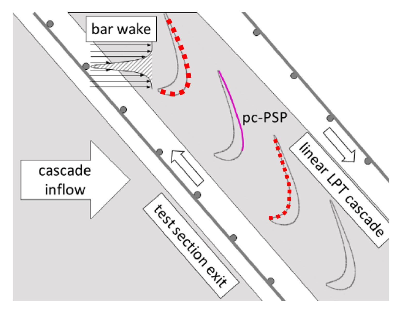
The time-resolved profile pressure measurements of the investigated LPT cascade were conducted in the High-speed Cascade Wind tunnel (HGK) located at the Institute of Jet Propulsion at the Universität der Bundeswehr Munich, Germany. The cascade consists of seven stator vanes. A general overview over the investigated geometry is displayed in
Figure 1. In contrast to the experimental setup of [
12] which focuses on the suction surface, two instrumented vanes are used in this research: One vane with 11 measurement positions on the suction and a second one with 13 positions on the pressure surface. For the measurements, these vanes are located adjacent to a central blade, each measuring the static pressure in the passage towards it. The location of the tappings, as well as their arrangement within the cascade is indicated by the red dots in
Figure 1.
The unsteady profile pressure is measured by fast-response pressure transducers of type
Kulite LQ-062 [
13] and is separated into its spectral components by means of Fourier-decomposition. The transducers are installed close to stator midspan where a two-dimensional flow is apparent. The transducers are incorporated from the backside into the vanes ensuring a high surface quality and avoiding disturbances of the flow by the large sensor screen. However, this leads to a cavity between measurement position on the surface and the sensor whose impact on pressure amplitude and phase must be taken into account. As discussed by [
12], the impact of the transfer function of the cavities is negligible at the investigated frequency. The phase lag due to the cavities’ lengths is considered. To achieve the best possible accuracy, all sensors are calibrated in MTU’s certified calibration facility.
Unsteady inflow conditions being representative for the wakes of an upstream located blade row are induced by the operation of a wake generator (WG) as proposed by [
14,
15]. The WG assembly consists of cylindrical steel bars of 2 mm diameter that are fixed on two moving belts. The belts move continuously in a loop with a constant circumferential speed providing a periodic inflow condition at a frequency of
500 Hz. A trigger signal linked to the WG is recorded allowing for a synchronization of its temporal position and the pressure transducers. Detailed information regarding the impact of the WG on the established flow field are given by [
16].
Although there are limitations in the rotational speed of the WG, the results are transferable to engine-like Strouhal numbers Sr and flow coefficients
[
17]. The flow condition at the inlet is determined by a total pressure level of
kPa and an inlet stagnation temperature of
K. The turbulence intensity of the inflow is raised to
by a turbulence grid installed in the upstream inlet nozzle. The assessed operating point corresponds to a Reynolds number of Re
60,000 and a Mach number of Ma
being representative for LPT conditions.
3. Evaluation Setup
In this section, a brief overview of the assessed numerical configurations is given. This includes a description of the applied flow solvers and a specification of the numerical setups. The flow field is determined by the solution of the compressible unsteady Reynolds-Averaged Navier–Stokes (URANS) equations. The physical state is described completely by the fluid density , momentum and the total energy .
The impact of turbulence is considered in accordance with Wilcox’
two-equation turbulence model [
18]. Although the flow around the moving WG is considered to be fully turbulent, the transition of the boundary layer from a laminar to a turbulent state is considered over the cascade surface by a correlation-based transition model [
19].
The evaluated solver methods are part of the CFD code framework TRACE which is developed at the Institute of Propulsion Technology at the German Aerospace Center DLR, Cologne, in cooperation with MTU Aero Engines AG, Munich. TRACE is a hybrid solver for the finite-volume discretization of the compressible URANS equations on both structured and unstructured grids in the relative frame of reference [
20]. It enables a nonlinear and unsteady analysis of three-dimensional turbomachinery flows in the time and the frequency domain in a parallel fashion exploiting hybrid distributed-/shared-memory structures.
Inviscid fluxes are treated by second-order accurate Roe upwind spatial discretization. The upwind states are considered by application of monotonic upwind schemes for conservation laws (MUSCL) [
21]. To avoid unphysical oscillations in the presence of shocks, a modified van Albada limiter [
22] is applied. The discretization of viscous flow components is realized via second-order accurate central difference schemes. The impact of turbulence can be considered by a various number of turbulence and transition models [
23] integrated in the code.
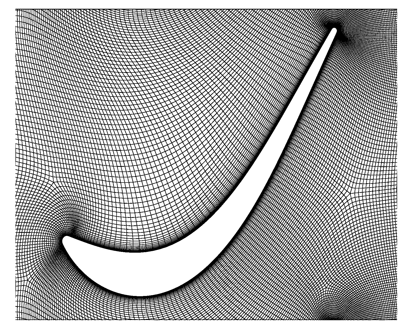
For the measured vane span, the spanwise flow components are of negligible order providing a nearly two-dimensional flow state. Therefore, the applied computational domain is reduced to only 5 cells in spanwise direction with symmetry conditions imposed on the spanwise boundaries. The numerical mesh discretizes the geometry of two WG passages and three stator vane passages, respectively. The resulting quasi three-dimensional mesh consists of ∼800,000 cells and relies on a block-structured grid topology as displayed in
Figure 2 for one LPT stator. The boundary layers around the WG surfaces are resolved by a dimensionless wall distance
of
forcing the application of wall functions there. In the stator cascade, a wall distance of
is never exceeded avoiding the usage of wall functions at the measured surface. The dependency of the results regarding a refinement of the mesh has been checked and found to be of negligible order.
For all simulations, equivalent boundary conditions are imposed. The boundary conditions are of non-reflecting type as proposed by [
24] and based on a formulation in the frequency domain as described by [
25]. At the inlet boundary, constant values of stagnation pressure
, stagnation temperature
and pitchwise flow angles are prescribed according to inflow measurements. Furthermore, constant inlet values for turbulence intensity Tu and length scale
are imposed in accordance with the installed turbulence grid. To reproduce the measured performance point, a constant static pressure level as met during the test is imposed as outlet boundary condition.
3.1. Setup for the Unsteady Simulations in the Time Domain
The mutual communication between the adjacent domains of the rotating WG and the non-rotating stator vane is realized by exploiting a zonal interface as described by [
26]. The simulations are performed by resolving a complete revolution of the two WG passages with 256 physical timesteps. This enables at least 128 physical timesteps per generator bar passing and 85 physical timesteps per vane passing, respectively. The underlying time-integration is based on a backward Eulerian scheme of second order. Within each physical timestep, a relaxation in pseudo-time related to an implicit Gauss-Seidel method with multiple solver sweeps is applied. To provide a periodic state at the end of the simulation, convergence is assessed according to [
27]. The simulation is stopped after 20 complete revolutions of the rotating WG domain.
3.2. Setup for the Harmonic Balance Simulations in the Frequency Domain
The consideration of the respective sources of unsteadiness appearing at differing frequencies and inter blade phase angles (IBPA) is treated by employing the harmonic set approach as proposed by [
4]. Each unsteady interaction between the adjacent computational domains is associated to an explicit combination of a base frequency and an IBPA. Since the higher harmonics of these interactions are defined as integral multiples of the respective combinations of base frequency and IBPA, they can be summarized in a so-called shared harmonic set (HS). The communication enabling the unsteady interaction between the adjacent domains is realized via a transfer of the harmonic content in each considered HS. The resolved harmonic sets, namely their base frequencies and their associated harmonics are summarized in
Table 1.
The dominant source of unsteadiness within the measured stator cascade (V1) is induced by its operation in the wake of the upstream located wake generator (WG). The harmonic content linked to the wake generator passing frequency (WGPF) is resolved by taking into account 10 harmonics and represented by a shared HS denoted in the following as HS
. The unsteady interaction between wake WG and potential field of the downstream stator cascade at the passing frequency of V1 (VPF
) in the rotating frame of reference is provided by HS
by resolving 4 harmonics. All considered harmonic content is coupled with the time-averaged flow field as indicated by the zeroth harmonic entries in
Table 1.
Two harmonic balance approaches differing in the treatment of turbulence are assessed in this work. One approach considers only the temporal average of the applied
turbulence model. This means that the flow fields of turbulence kinetic energy
k and dissipation rate
are only solved for their Reynolds-averaged components
and
Formulating this approach in terms of the frequency domain, this is equivalent to a consideration of only the zero harmonic component of the turbulence quantities k and . Therefore, this approach is in the following also denoted as HB- since it includes only a time-invariant information of the eddy viscosity .
The second HB approach resolves the unsteady turbulence components
and
by the number of harmonics listed in
Table 1. As explained in the following and motivated in [
8,
11], the HB method is then prone to numerical instabilities induced by the unsteady consideration of the turbulence model. Thus, this HB approach requires the application of a Lanczos-type filter method and is therefore in the following abbreviated with HB-
.
3.3. The Lanczos-Filter Method
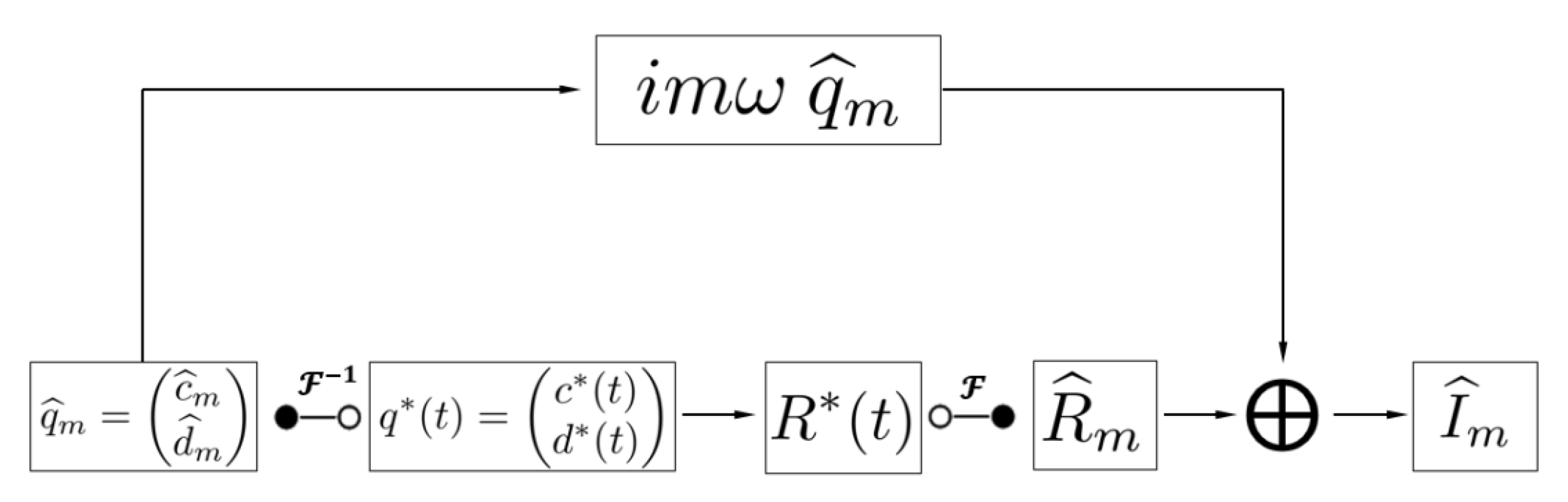
The HB method realized in the applied flow solver TRACE relies on a hybrid frequency-time-domain approach as described in [
3]. As displayed in
Figure 3, the nonlinear contributions
of the URANS equations are provided in the frequency domain by relying on a transformation from frequency to time domain and vice versa.
Based on the harmonic content of a previous iteration step, the flow field is first reconstructed in the time domain for a defined set of N sampling points. This is achieved by performing an inverse discrete Fourier transform. Hence, for each of the predefined N sampling points, information about the complete flow field is available. Accordingly, the associated nonlinear contribution can be calculated for each of the N sampling points in time. In a subsequent step, a discrete Fourier transform over all stored in each of the N sampling points is performed providing the required nonlinear component in the frequency domain.
The basic idea behind the application of any frequency domain method as the HB approach is to take advantage of model order reduction by focusing on a limited number of frequencies and associated harmonics. Since the number of considered harmonics is highly limited, the reconstruction from frequency to time domain suffers always to a certain extent from the Gibbs phenomenon. Quantities linked to turbulence modeling—that is turbulence kinetic energy
k and dissipation rate
— are affected by this in the most critical order as discussed by [
8].
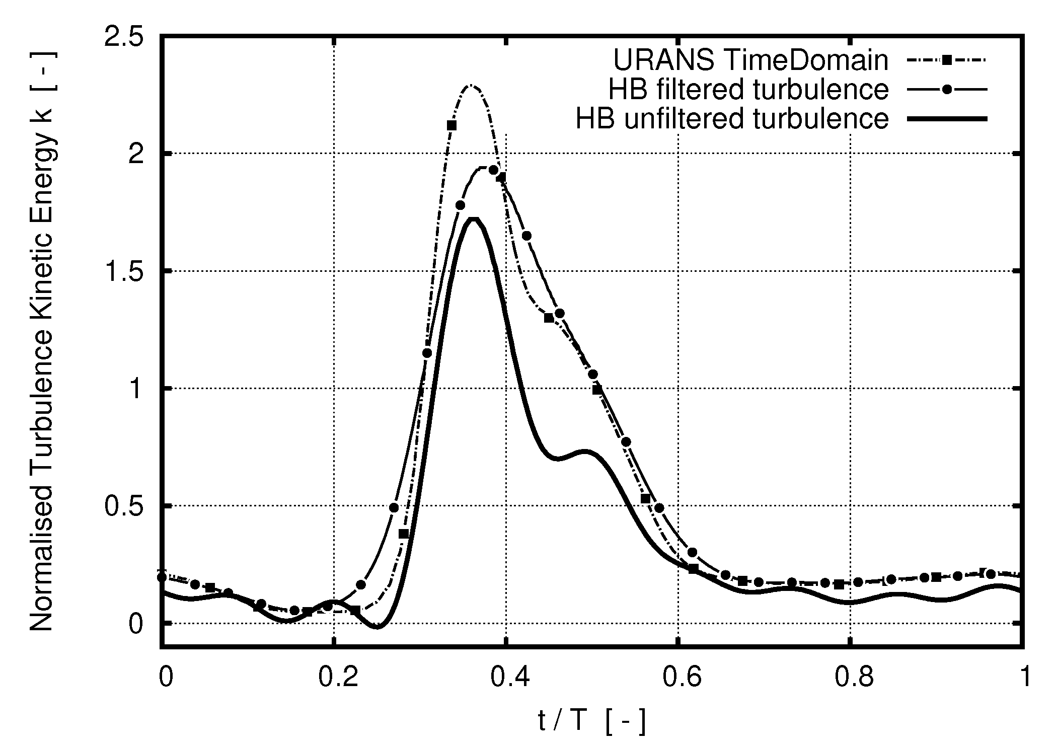
The ringing associated with the Gibbs phenomenon causes undershoots for
k and
potentially leading to negative values for these quantities. This is highlighted in
Figure 4, where the turbulence kinetic energy
k downstream of a LPT stator vane is plotted over one blade passing period
T. The dash-dotted line in
Figure 4 displays the reference result from a time-marching URANS simulation which indicates high levels of turbulence kinetic energy
k in the presence of the wake between
. In the freestream region of the stator exit, the level of turbulence fluctuation turns out to be close to zero.
The equivalent wake resulting from a HB simulation operating with a limited number of harmonics is represented in
Figure 4 with a solid line. The negative impact of Gibbs phenomenon becomes obvious in regions close to high gradients as in the appearance of the wake. The undershoots caused by the Gibbs phenomenon lead to approximations of
k with very low or even negative values. From a physical point of view, this is not feasible since
k is a quantity defined as solely positive. In the context of turbulence and transition modeling, operating with values close or even out of the defined range affects both the reliability and the stability of the underlying numerical algorithms in a very unfavorable fashion. Hence, unsteady turbulence effects have been neglected in previous HB studies by exploiting a frozen eddy viscosity approach [
9].
However, the negative impact of the Gibbs phenomenon in the presence of high gradients can be alleviated by the application of Lanczos-type filter methods as proposed by [
8,
28,
29]. In practice, the application of the Lanczos-filter can be realized via a multiplication of the Fourier coefficients of the respective turbulence quantities with the Lanczos-
factors
Here,
m represents the respective harmonic degree while
M denotes the truncation order. Detailed information regarding theory and its computational realization can be found in [
8].
According to
Figure 4, the wake predicted by the Lanczos-filtered HB-
approach is displayed by a solid line with dots. The solution of the HB-
method shows no critical undershoots near the wake while the level of turbulence kinetic energy
k is maintained in the freestream region. However, the wake’s shape is predicted to be wider and its peak to be lower if the Lanczos-filter method is applied. Both observations are not surprising since the increase of stability due to the filter happens at the expense of the capability to capture sharp gradients. This is the case for all blurring-type filters.
Therefore, the question arises if the application of the Lanczos-filter method affects the capability of the HB- method to predict the unsteady pressure fluctuations in an ineligible fashion. This is discussed in the remainder of this work.
This is achieved by comparing the results of the HB- approach to measurement data, as well as to reference results generated by a time-marching URANS simulation and to the HB- method. Since the HB setup defined above suffers from the destabilizing Gibbs phenomenon in a way that makes a solution without filter application impossible, a validation against an unfiltered HB approach is not possible in this work.
4. Results and Discussion
The results of the respective numerical solution approaches regarding the unsteady pressure fluctuation are compared to the unsteady measurement data. Therefore, the pressure fluctuation amplitude—normalized by the leading edge’s stagnation pressure—is plotted for the respective approaches in
Figure 5. The results are displayed along the axial chord length
at the midspan of the stator cascade. The stator’s pressure side is displayed from
while the results associated with the stator’s suction side are plotted in the range between
. Accordingly, the stagnation point and the leading edge of the profile, respectively, are marked by
while the profile’s trailing edge is determined by
. The focus of this research is exclusively on an assessment of the frequency linked to the first WGPF harmonic.
In
Figure 5, the reference relying on the unsteady fast-response measurement data are plotted with filled squared symbols while the benchmark results generated by the time-integration method are represented by a dashed line. The results of the filtered HB-
approach are displayed with a solid line. Finally, the results of the HB-
method are added to
Figure 5 by a solid-dotted line.
Focusing on the results for the pressure side in the range from , a remarkable agreement of the time-integration and the HB- method with the measurement data can be observed. Both methods can reproduce the fluctuation amplitude induced by the WG in both quality and quantity. Differences appear increasingly in regions closer to the trailing edge. The prediction of the time-integration and the filtered HB- method match over the complete pressure side. The HB- approach shows in return a significant though rather constant offset over the profile’s pressure side. The qualitative behavior of the fluctuation amplitude, however, is captured very well.
Looking on the suction side, again the time-integration and the filtered HB- approach agree over a substantial region of . In this region, the numerical results are supported by a satisfying agreement with the measurement data. As for the pressure side, the HB- approach overestimates the pressure fluctuation amplitude in this part of the suction side while still being able to capture the qualitative behavior in a suitable manner.
Further downstream at , the deviations of the assessed approaches in both quality and quantity become more apparent. Although all numerical approaches overestimate the pressure fluctuation amplitude compared to the measurement data, the results of the time-integration solver reproduce at least qualitatively the measurement. In particular, the time-integration method proves to be the only one indicating a substantial fluctuation peak towards the trailing edge at . However, both decline of the fluctuation amplitude between as its subsequent rerise between are underestimated by the time-integration method.
Although the tendency of a raise in the predicted pressure fluctuation amplitude can be observed for the results of both investigated HB methods, this behavior is limited to a very short region in the case of the HB- solver. Although the HB- method predicts this rerise over a wider part of the stator in the region between , its peak appears to be of substantially lower order and by a much smaller gradient if compared to the transient measurement data and the time domain solution, respectively.
Recalling the sufficient agreement for the pressure side and the upstream part of the suction side, this hints at a differing prediction of the transition from a laminar to a turbulent state of the underlying boundary layer. To judge potential differences regarding the predicted transition behavior, the shape factor
defined as
is assessed for the respective solution approaches. Here,
denotes the displacement thickness and
the momentum thickness of the boundary layer.
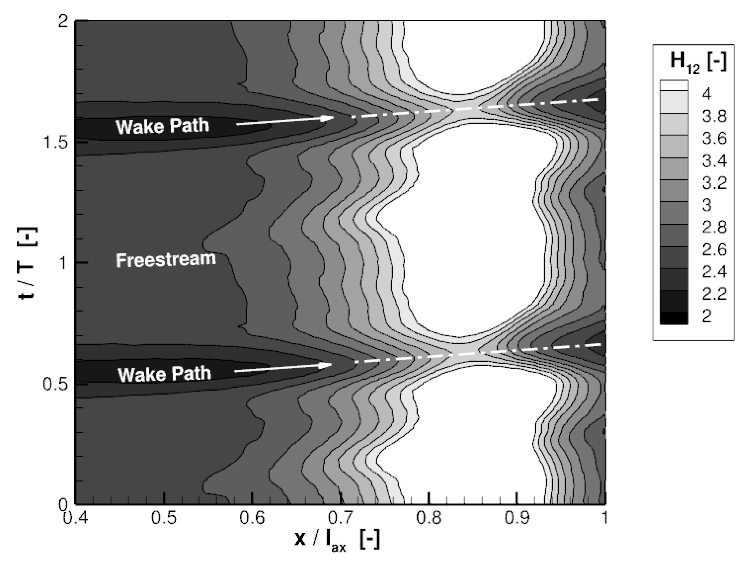
In
Figure 6 and
Figure 7, the space-time diagrams of the shape factor
are displayed for two WG passings
T. The focus is on the suction side in the range between
. The results of the time-integration method are shown in
Figure 6 and indicate a transition behavior alternating between separation induced transition at freestream and bypass induced transition at wake conditions, respectively. The flow separation at freestream condition marked by high values of the shape factor
between
is completely suppressed in the presence of the passing wake. This is highlighted by low levels of
at
resulting in a subsequent reattachment. The reattachment appears as a consequence of an increased turbulence level induced by the upstream located WG. This behavior is in-line with the findings of [
12] where a separation bubble pulsating with the WGPF could be identified by means of pressure-sensitive paint.
The results of the Lanczos-filtered HB-
method are shown in
Figure 7. The presence of the flow separation is predicted reliably in general. However, the suppression induced by the passing wake though present is not causing a complete reattachment neither it affects a region of same order. In fact, the significant increase of the pressure fluctuation amplitude between
coincides for both solution methods with the region of flow separation identified in
Figure 6 and
Figure 7.
Consequently, the impact of the unsteady transition behavior dominates in the presence of separation induced transition the excitation behavior completely. However, all applied numerical solution methods suffer to a certain extent from an underestimation of the separation induced excitation. Nevertheless, this raises the question about the HB method’s capability to predict the unsteady transition behavior and to which extent it is affected by the application of the assessed Lanczos-filter approach.
In recent studies of [
10], the general capability to predict the unsteady transition if the Lanczos-filter method is applied, has been investigated. This is achieved by comparing time-resolved measurement data conducted by surface thin film gauges within a 2-stage LPT test facility. The results presented in [
10] support the harmonic balance general capability to reflect the unsteady transition behavior while taking advantage of the Lanczos-filter approach. However, in contrast to the pure correlation-based transition model applied in this effort, transition is modeled in [
10] by relying on the solution of two additional transport equations. As usual in the context of Menter’s
framework [
30], one equation represents the intermittency
and the second models the transition Reynolds number
. It is neither new nor surprising that a hybrid frequency-time domain approach, as the Harmonic Balance method applied in this work, suffers if transition modeling is considered based on pure correlation. In fact, the treatment of the transition modeling in the frequency domain in an equivalent fashion turns out to be difficult.
However, the transition model based on the work of [
19] proves to be the only one being able to predict the presence of the separation bubble for the investigated LPT-geometry. Therefore, a separated discussion of the differences induced by the Lanczos-filter method and by the differing treatment of the underlying transition model is not possible in this work.
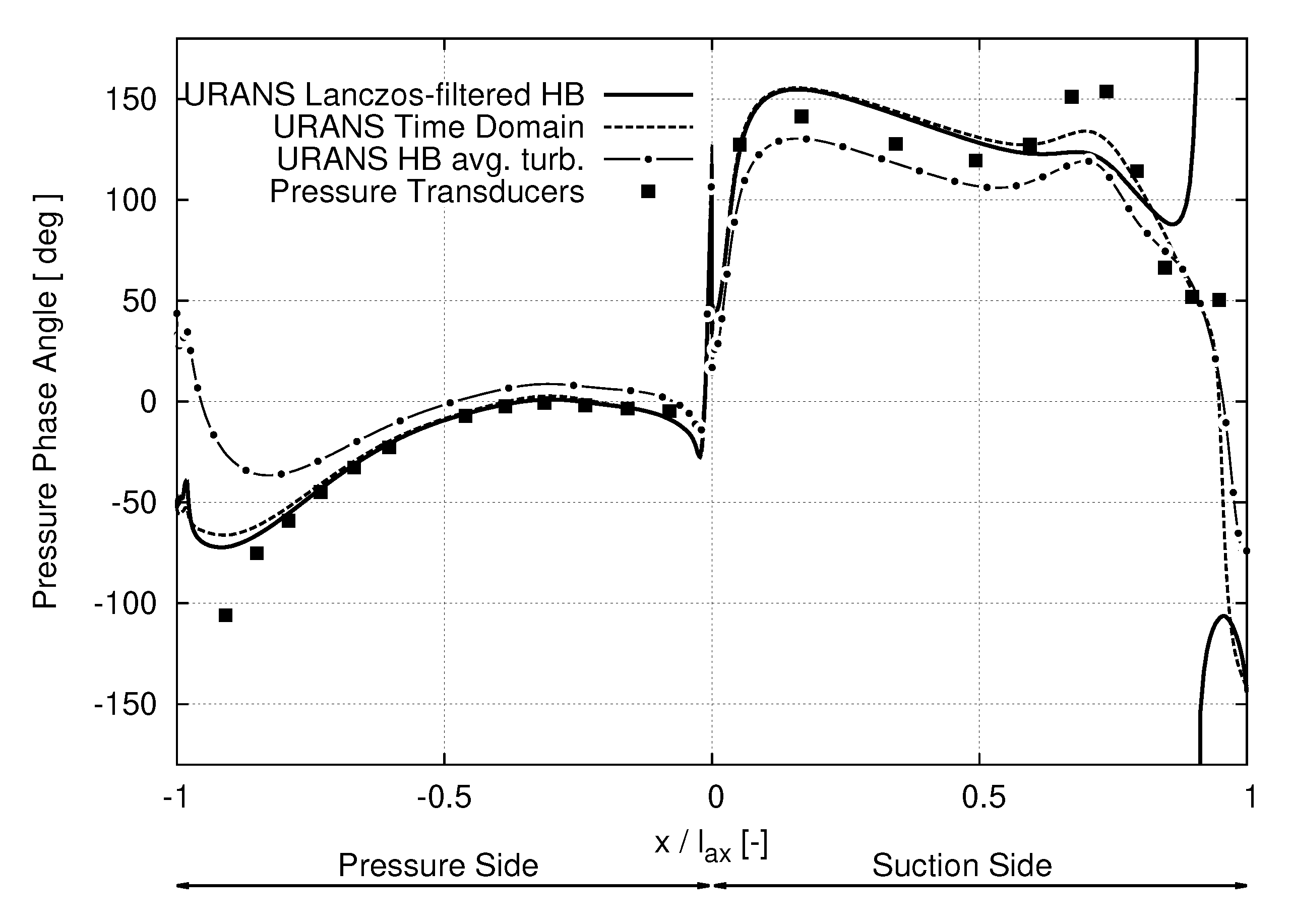
In terms of forced response driven excitation, the reliable prediction of the pressure fluctuation’s phase relation is of same importance as its associated amplitude. Therefore, results of the fluctuation phase relation are plotted in
Figure 8. The numerical results for both the pressure and the suction side are synchronized in accordance with the recorded trigger signal linking the WG start position to the pressure tappings. As already noticed for the fluctuation amplitude, all investigated numerical approaches can reproduce the phase relation over vast parts of the pressure side between
. Again, the HB-
approach indicates a constant phase shift of approximately
. However, all predictions of the fluctuation phase relation differ increasingly and substantially by proceeding further downstream towards the pressure side’s trailing edge at
.
Finally, the results of the fluctuation phase angle linked to the suction side of the investigated stator cascade differ quantitatively for all presented solution approaches though the qualitative behavior is reproduced sufficiently for the front part up to . Again, the results of the time-integration and the HB- method match in this region while the HB- solution shows an offset in an order of . Since the measurement indicates values in between, all simulations suffer from a shift in an order of approximately in this region though.
As previously stated, the rear part of the suction side at is highly dependent on the presence of the separation behavior. This results in substantial deviations of the fluctuation phase angle in this region as well. The time-integration method reproduces the best approximation of the phase relation. Although the HB method neglecting unsteady turbulence differs massively from the measurement data, the HB approach considering the turbulence’ unsteadiness is not able to reflect the sharp local rise and decrease in the presence of the separation sufficiently.
Coming closer to the suction side’s trailing edge, the agreement of the predicted phase relations with the measurement data decreases further which makes a reliable assessment of the results difficult in this region. This is in particular the case for the HB-
approach indicating a rise of the phase angle at
. This hints again at an insufficient prediction of the spatial and temporal propagation of the separation bubble in the HB-
approach as apparent in
Figure 6 and
Figure 7. In fact, the measurement data indicate its impact to be more distinct and to be located further downstream. To improve the quality of the Lanczos-filtered HB-
method, it is mandatory to consider the unsteady transition behavior in a more reliable fashion than it is possible at this stage.
The benefit of model order reduction approaches as the assessed HB method consists of a more time-efficient and less time-consuming solution approach. Accordingly, the quality of the provided results must be related to the underlying numerical costs of the respective approaches. The computational efforts required by the methods are summarized in
Table 2. Generating the results by relying on the time-integration method leads to highest requirements regarding CPU- and total wall-time. Compared to the effort linked to the HB-
method, the numerical costs turn out to be of factor 2 higher. The HB-
approach provides a compromise between both methods. Resolving during the HB-
solution the equations for turbulence kinetic energy
k and dissipation rate
in an unsteady framework raises the numerical effort in an order of 50%.
However, the investigated two-dimensional evaluation setup favors the time-integration method in a disproportional order. Blade counts in real engine-like problems often force the consideration of half- or even full-wheel configurations for the time-stepping method—which is not the case for the HB approach. Therefore, for real three-dimensional engine applications, the numerical effort required by the time-integration method turns out to be ∼20 times higher than in HB, as stressed for instance by [
10].


 ,
, 


