Article

Multi-Channel High-Dimensional Data Analysis with PARAFAC-GA-BP for Nonstationary Mechanical Fault Diagnosis

1
Wuhan Institute of Technology, School of Mechanical and Electrical Engineering, Wuhan 430074, China
2
Nanchang Institute of Science and Technology, School of Artificial Intelligence, Nanchang 330108, China
*
Author to whom correspondence should be addressed.
Int. J. Turbomach. Propuls. Power 2022, 7(3), 19; https://0-doi-org.brum.beds.ac.uk/10.3390/ijtpp7030019
Submission received: 1 February 2022 / Revised: 23 April 2022 / Accepted: 3 May 2022 / Published: 28 June 2022

Abstract

:
Conventional signal processing methods such as Principle Component Analysis (PCA) focus on the decomposition of signals in the 2D time–frequency domain. Parallel factor analysis (PARAFAC) is a novel method used to decompose multi-dimensional arrays, which focuses on analyzing the relevant feature information by deleting the duplicated information among the multiple measurement points. In the paper, a novel hybrid intelligent algorithm for the fault diagnosis of a mechanical system was proposed to analyze the multiple vibration signals of the centrifugal pump system and multi-dimensional complex signals created by pressure and flow information. The continuous wavelet transform was applied to analyze the high-dimensional multi-channel signals to construct the 3D tensor, which makes use of the advantages of the parallel factor decomposition to extract feature information of the complex system. The method was validated by diagnosing the nonstationary failure modes under the faulty conditions with impeller blade damage, impeller perforation damage and impeller edge damage. The correspondence between different fault characteristics of a centrifugal pump in a time and frequency information matrix was established. The characteristic frequency ranges of the fault modes are effectively presented. The optimization method for a PARAFAC-BP neural network is proposed using a genetic algorithm (GA) to significantly improve the accuracy of the centrifugal pump fault diagnosis.

1. Introduction

Mechanical equipment plays a significant role in the construction of the national economy and is an integral part of the entire industrial sector [1]. With the great developments in the improvement of modern production that have taken place, the structures of modern equipment are becoming much more complex. The mechanical equipment needs to remain resilient in severe working conditions. Due to the influence of many unavoidable severe environmental factors, machinery and equipment such as the centrifugal pumps, gearboxes, engines, and other major components that work under a heavy load, high temperature and high pressure experience a variety of the failures. Especially given the extension in their working life, the mechanical components inevitably suffer aging, wear, tear, etc. If failure in the machinery and equipment is not handled promptly, minor damages progress to severe failures, which delays production, causes huge economic losses and serious accidents that endanger the lives of staff [2]. The timely prevention of mechanical equipment failure to maintain the safe operation of equipment in industrial production is of paramount importance.
Centrifugal pumps have excellent properties such as a simple structure, high efficiency and stable performance. They are widely used in industrial production. It is necessary to diagnose and monitor the running status of the centrifugal pumps during the complex industrial process such as in the oil industry, etc. [3]. The current mainstream vibration signal-based centrifugal pump fault diagnosis method mainly relies on machine learning [4]. Reference [5] selects the time-domain characteristic signal of an electrical submersible pump using the decision tree algorithm and inputs it into a classifier to realize fault separation. Studies in the literature [6] introduce the idea of the k-nearest neighbor algorithm into traditional Markov distance fault judgment to forecast three common centrifugal pump faults. Bordoloi D J et al. used support vector machines to effectively diagnose the blockage level and obstruction cavities at different pump speeds [7]. In the context of Industry 4.0, given the progress in computer science, sensors, cloud technology, big data, etc., the large scale of data collection and the storage of the complex industrial systems are becoming easier and the scale of data is becoming larger, which characterizes the structure of data as high-dimensional. Currently, the processing of high-dimensional data from the large scale industrial processes, which are used to mine valuable information, is a hot topic in the literature [8].
Traditional data-processing methods have a great capability of reducing the dimension of data, such as the Principal Component Analysis (PCA), Intrinsic Modal Analysis (EMD), Wavelet Packet Energy (WPE) and local characteristic analysis (LFA) [9]. Combining the above dimensionality reduction method with a neural network to process massive data and realize data mining has become the mainstream research direction in the research community [10]. C Cui constructed the PCA-BP-MSET model to achieve effective fault warning in an air compressor fault diagnosis system [11]. For abnormalities in the sensor system, Yu used EMD to process the data and PNN as a classifier to achieve fault classification [12]. Compared with the above algorithms, the parallel factorization processing tensor has the advantage of reducing data loss and computational complexity because the tensor represents the properties of the higher order data without damaging the intrinsic structure and underlying information of the data. One of the most promising theories of parallel factorization comes from Kruskal and the new concept of k-order [13]. The k-order for matrix A is the maximum that satisfies the condition that any k column vectors of the matrix A are uncorrelated linearly, which reveals sufficient conditions for the application of the parallel factorization method and lays foundations for its applications in signal processing [14]. Zhang et al. applied PARAFAC decomposition for radar spatial-temporal signal processing to achieve the automatic angle and frequency matching [15]. Li et al. [16] used the parallel factor analysis to deal with the separation of multiple fault sources in the mechanical equipment and achieved the desired results. Sidiropoulos et al. used PARAFAC analysis for the recognition and identification of multiple targets in MIMO radar systems [17]. Weis et al. used the PARAFAC algorithm in their EEG data analysis to determine the individual components of the correlation [18]. Yang et al. constructed tensor using wavelet transform and processed multi-dimensional fault signals with parallel factor theory to achieve effective classification [19].
Genetic algorithm (GA) comes from the idea and mechanism of natural evolution as the optimal parallel search in the laws of biology. It is constructed by simulating the principle of “natural selection and survival of the fittest” in the natural evolutionary process. GA provides a solution to complex nonlinear problems that are not easily solved by the traditional optimization methodology [20]. A genetic algorithm was proposed for combination with the support vector machine (SVM) to achieve the optimal algorithm for fault diagnosis of the rolling bearing machines [21]. The ICA algorithm was implemented for the feature extraction of the signal in the motor bearing, which is combined with GA to optimize the radial basis neural network for fault diagnosis. The diagnostic accuracy was significantly improved [22]. Compared with the traditional neural network (NN), the optimized and improved NN has an optimal network structure and higher accuracy.
This paper investigates the relevant theory relating to signal matrix decomposition and applies continuous wavelet transformation to multi-channel signal analysis to construct a three-dimensional tensor. The parallel factor decomposition achieves the characteristic information extraction of the complex systems, which determine the frequency range of the faulty centrifugal pump. The effective feature frequency information extraction is combined with the excellent adaptive updating ability and nonlinear characteristics of BP-NN. The BP-NN model is established to diagnose the fault modes of the centrifugal pump. In order to overcome the disadvantage of the slow convergence of the BP-NN, the optimization method based on GA is proposed to optimize the BP neural network model so that it finds the appropriate weights and thresholds at a quicker rate and rapidly achieves fault classification.

2. Principle of Parallel Factor Analysis

Tensor is the high-dimensional form of data construction. The dimensionality of the data is called the order of the tensor and is considered the generalization of the matrix and vector in the high-dimensional spatial construction. Traditional methods such as ICA, PCA, etc. used for processing data with high dimensionality generally spread the data into a two-dimensional matrix for processing to remove the structural data. The solution often fails to achieve the expected results. PARAFAC is a common decomposition treatment in tensor decomposition. The core idea is to approximate the original tensor data by the sum of finite rank-1 tensors.

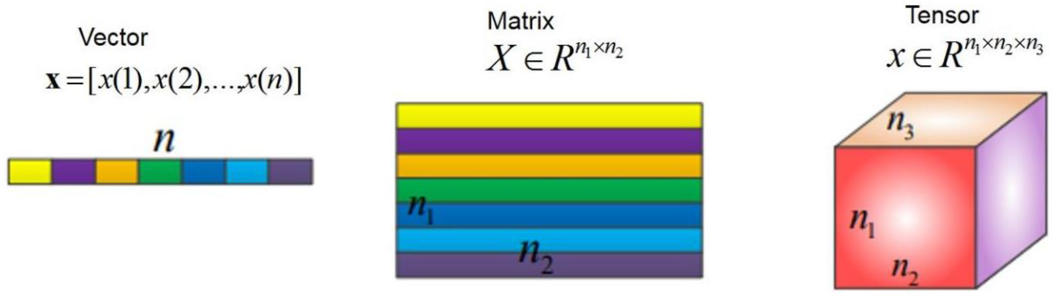
2.1. Parallel Factor Model

Tensor is a high-dimensional extension of the matrix. The order of the tensor represents the dimensions of the tensor as shown in Figure 1. The vector formed by the one-dimensional time series of the vibration signal collected by the single-channel sensor is the 1 st order tensor. The matrix is the 2nd order tensor. The multi-dimensional array above the three-dimensional level is the high-order tensor.
In the two-dimensional matrix, the variable x p , q generally is applied to indicate the components of the two-dimensional matrix that the subscript denotes the x-axis and the subscript q denotes the y-axis during the x y 2D coordinate system. The variable x p , q , k indicates the element of the three-dimensional matrix that the subscript p denotes x a xis, subscript q denotes y axis and subscript q denotes z a xis during the x y —z 3D coordinate system. The 2-D array of the 3D matrix constitutes the subarray of the 3D matrix. The subarray is labeled as the slice of the 3D matrix in the axis. The low-rank decomposition of the matrix is extended to construct the 3D matrix. Let the variable x p , q , k be the elements of the three-dimensional matrix X C P × Q × K , where p = 1 , , P ; q = 1 , , Q ;   k = 1 , , K . Three-dimensional matrices can be represented as vector outer product as follows:
X = a 1 b 1 c 1 + , , + a R b R c R = r = 1 R a r b r c r
where a r C P b r C Q c r C K r = 1 , 2 , , R . Equation (1) provides the low order decomposition process of the 3D matrix. The orders of the 3D matrices X are R . The model for the low-rank decomposition of the 3D matrix as shown in Equation (1) is Parallel Factor Model. Figure 2 shows the procedure of the PARAFAC model.
Here, the definitions of the three matrices are as follows:
A = [ a 1 , , a R ] B = [ b 1 , , b R ] C = [ c 1 , , c R ]
The symbols A, B, and C are the three loading arrays in the PARAFAC model. Equation (2) shows that the components in the 3D array X are decomposed as the sum of the multiplication of R components.

2.2. Uniqueness of Parallel Factor Decomposition

For a two-dimensional matrix, when the rank of the matrix is greater than 1, the two-dimensional matrix’s low-rank decomposition is not unique if there are no special structural constraints. For the matrix decomposition process X = ABT, there exists another set of matrices A ¯ , B ¯ that is X = A B ¯ T . However, A ¯ A Π A Δ A , B ¯ B Π B Δ B , Here, the symbols Π A and Π B are column swap matrices and the symbols Δ A and Δ B are the diagonal scale matrices. The uniqueness of the two-dimensional matrix decomposition is illustrated by the converse method. Given any full-rank approach T C F × F with
X = A B T = A T T 1 B T = A B ¯ T
Among them
A ¯ = A T = [ a ¯ 1 , , a ¯ F ]
B ¯ = B ( T 1 ) T = [ b ¯ 1 , , b ¯ F ]
where a ¯ f and b ¯ f are the column vectors of the arrays A and B. If the arrays A, B are full rank, A ¯ and B ¯ are also full rank matrices, then we have
X = A B ¯ T = a 1 ¯ b 1 T ¯ + a 2 ¯ b 2 T ¯ + + a F ¯ b F T ¯
The above formula satisfies the definition of the low order decomposition. However, T Π Δ . Therefore, the 2D matrix low-rank decomposition is not unique.
The fundamental difference between the parallel factorization and the 2D matrix decomposition is the uniqueness of its decomposition, which is one of the reasons that the PARAFAC model is widely used in data analysis. The uniqueness theorem of PARAFAC decomposition comes from the new concept of the k-order. The k-order for a matrix A is the maximum order of k and satisfies the condition that any k column vectors of the array A are linearly uncorrelated, which reveals the sufficient conditions for the uniqueness of the parallel factorization method for application in data analysis. Consider the sub-profile matrix of the PARAFAC model along the X-axis.
X P Q × K = B D p ( A ) C T p = 1 , 2 , , P
Here, the matrix is A R P × R , B R Q × R , C R K × R , if the following inequality is satisfied
k A + k B + k C 2 ( R + 1 )
The matrices A, B, and C are unique.

3. Hybrid Method with PARAFAC_GA_BP_NN

3.1. Algorithm on PARAFAC

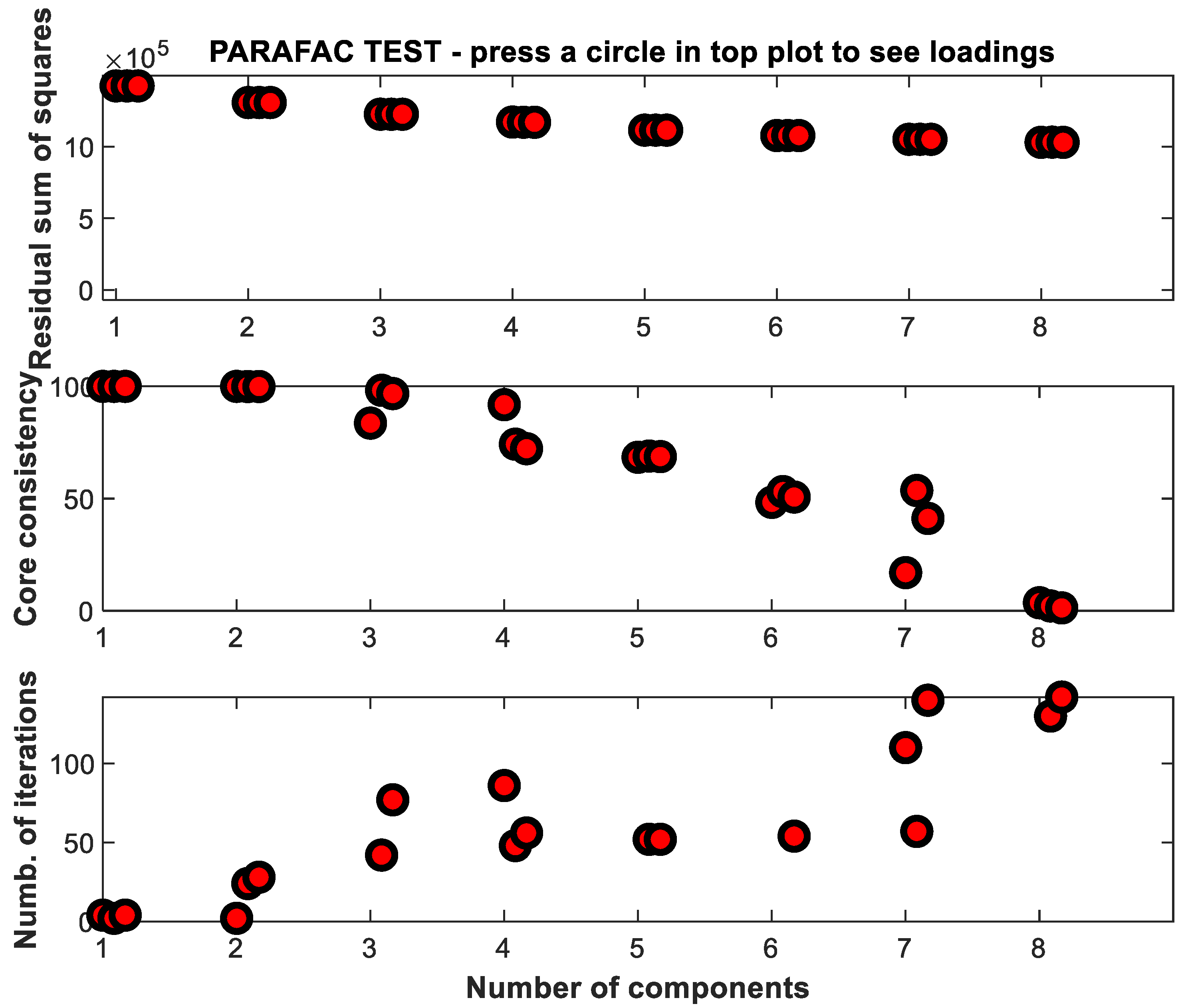
3.1.1. Nuclear Consistency Estimation

The PARAFAC algorithm is very sensitive to the pre-estimated factor F. When the parameter F is estimated as too low, no physically meaningful solution is obtained. If the parameter F is estimated as too high, it leads to an increase in the model error and makes the deviation between the calibration values and the true values larger. Therefore, a suitable value for factor F is very important for constructing the PARAFAC model. It is necessary to pre-estimate the number of factors. Since the ranks of the tensors are obtained asymptotically, different methods are usually used to evaluate the decomposition factor number from several perspectives. Here, Core Consistency estimation is an effective methodology for the estimation of the factors by calculating the level of the similarity between the super-diagonal array T and the core 3D data array G in the PARAFAC model. The calculation of Core Consistency ( δ ) is defined as follows:
δ = 100 × ( 1 d = 1 F e = 1 F f = 1 F ( g d e f t d e f ) 2 F )
where the parameter F is the factor number in the PARAFAC model, the parameter g d e f is the element of the matrix G, the parameter t d e f and is the element of T. For the ideal PARAFAC model, the superdiagonal arrays T and G should be very similar, at which point the kernel agreement value equals 100%. Usually, when the kernel agreement value is equal to or more than 60%, the model is considered to be close to trilinearity. However, when the kernel agreement value is lower than 60%, the model is considered to deviate from trilinearity. A much more accurate factor number is obtained according to the change in the kernel agreement value.

3.1.2. Trilinear Alternating Least Squares (TALS)

| X p q k | is an arbitrary three-dimensional data set. The two-dimensional matrices defined as X p ( Q × K ) , X q ( P × K ) and X k ( P × Q ) that the corresponding elements satisfy the following conditions.
X p ( q , k ) = X q ( p , k ) = X k ( p , q ) = X p q k
Then, the three-dimensional matrix is described as the joint cubic equation along the three different dimensions.
{ X p = B d i a g ( A ( p , : ) ) C T , p = 1 , 2 , , I X q = C d i a g ( B ( q , : ) ) A T , q = 1 , 2 , , J X k = A d i a g ( C ( k , : ) ) B T , k = 1 , 2 , , K }
where the variables X p X q and X k denotes the slice of the three-dimensional matrix X in the three directions P , Q and K. The symbol d i a g ( A ( k , : ) ) denotes the square matrix after the diagonalization of the k th row elements of the matrix A and so on from Equation (11).
[ B d i a g ( A ( 1 , : ) ) C T C d i a g ( B ( 2 , : ) ) C T A d i a g ( C ( I , : ) ) C T ] = [ B d i a g ( A ( 1 , : ) ) C d i a g ( B ( 2 , : ) ) A d i a g ( C ( I , : ) ) ] C T = [ X i = 1 X i = 2 X i = I ] = X P Q × K
[ B d i a g ( A ( 1 , : ) ) C d i a g ( B ( 2 , : ) ) A d i a g ( C ( I , : ) ) ] = A B
Then, the PARAFAC model is expressed in the form of the Khatri-Rao product.
X P × Q K = A ( B C ) T X Q × K P = B ( C A ) T X K × P Q = C ( A B ) T
The basic idea of the TALS method is to update one array at one step by initializing a matrix and updating the remaining matrices using the Least Mean Square (LMS) Method. This step is repeated until the algorithm converges.
The hypothetical 3D dataset X with the dimensions P × Q × K is represented by a trilinear model in the following form.
x p , q , k = f = 1 F a p , f b q , f c k , f + e p q k p = 1 P q = 1 Q k = 1 K
Here, the symbol F denotes the number of components, the symbol a p , f is the p th component of the vector a f , the symbol b q , f is the q th component in the vector b f , the symbol c k , f is the k th component in the vector c f . The symbol x p , q , k   ( p = 1 , , P ,   q = 1 , , Q ,   k = 1 , , K ) . P × Q × K forms the three-dimensional space of the data set X. The symbol e p q k ( p = 1 , , P , q = 1 , , Q , k = 1 , , K ) is the error, which forms the 3D error set E on the P × Q × K coordinate system. The symbol A = [ a 1 , a 2 , , a P ] is defined as a P × F matrix. B = [ b 1 , b 2 , , b Q ] is a Q × F matrix. The symbol C = [ c 1 , c 2 , , c K ] is a K × F matrix.
Matrix A is calculated as:
[ X 1 X 2 X K ] = [ B d i a g C ( 1 , : ) B d i a g C ( 2 , : ) B d i a g C ( K , : ) ] A T + E K
Here, X k = B d i a g ( C ( k , : ) ) A T + E k , k = 1 , 2 , , K , E k is the error.
The least mean square estimate of the matrix A T is determined by the following equation.
A ^ T = [ B d i a g C ( 1 , : ) B d i a g C ( 2 , : ) B d i a g C ( K , : ) ] + [ X 1 X 2 X K ]
Here, [ ] + is the generalized inverse.
The matrix B is determined as:
[ Y 1 Y 2 Y P ] = [ C d i a g A ( 1 , : ) C d i a g A ( 2 , : ) C d i a g A ( P , : ) ] B T + E P
Here, Y p = C d i a g ( A ( p , : ) ) B T + E p , p = 1 , 2 , , P , E P is the error.
The least mean square estimate of the matrix B T is defined as:
B ^ T = [ C d i a g A ( 1 , : ) C d i a g A ( 2 , : ) C d i a g A ( P , : ) ] + [ Y 1 Y 2 Y P ]
The matrix C is determined as follows.
[ Z 1 Z 2 Z Q ] = [ A d i a g B ( 1 , : ) A d i a g B ( 2 , : ) A d i a g B ( Q , : ) ] C T + E Q
Here, Z q = A d i a g ( B ( q , : ) ) C T + E q , q = 1 , 2 , , Q , E Q is the error.
The least mean square estimate of the parameter C T is defined as:
C ^ T = [ A d i a g B ( 1 , : ) A d i a g B ( 2 , : ) A d i a g B ( Q , : ) ] + [ Z 1 Z 2 Z Q ]
Loop (1) to (3) are repeated, and the matrix is updated until convergence.

3.1.3. Algorithm Implementation of Parallel Factor Analysis

Each element X p q k of the tensor X P × Q × K consists of a trilinear component model as follows:
x p q k = f = 1 F a p f b q f c k f + e p q k
In signal processing, the parameter F contributes to the transient response signal, the variable a p f is the value of the f component related to the p th sample information, the variable b q f is the response value of the f th component related to the q th sample information, the variable c k f is the value of the f th component related to the k th sample information. The variables a p f , b q f and c k f are the components of the array A, B and C. The variable e p q k is the measurement error. The above equation is in the form of the PARAFAC model. It can be expressed in terms of three slice matrices that the trilinear model is expressed as in the following form, which is similar to the singular value decomposition in PCA.
X p ( Q × K ) = B d i a g ( a p ) C T + E p ( J × K ) , p = 1 , 2 , , P X q ( K × P ) = C d i a g ( b q ) A T + E q ( K × I ) , q = 1 , 2 , , Q X k ( P × Q ) = A d i a g ( c k ) B T + E k ( P × Q ) , k = 1 , 2 , , K
Here, the parameters a p , b q and c k are the p th row of the array A, the q th row of the array B and the k th row of the array C. The symbols d i a g ( a p ) , d i a g ( b q ) and d i a g ( c k ) are diagonal vectors of the F × F matrix. The parameters a i , b j and c k are the elements of the diagonal vectors. The symbol “T” denotes the transpose of the matrix. The variables E p ( Q × K ) , E q ( K × P ) and E k ( P × Q ) are three slices of the error array. Equation (22) is expressed as a matrix.
X = A T ( F × F F ) ( C B ) T + E
Here, the symbol is the Kronecker product, the array T ( F × F F ) is a two-dimensional matrix of the recombination of the core 3D data frame T. The variable T is a unit diagonal 3D-data array (also called a super diagonal array) with the matrix size ( F × F × F ) where the super diagonal element equals 1 and the remaining elements are zero.
In the standard PARAFAC model, the sum of squared residuals (SSR) is the minimization of the loss function, which is defined as:
S S R = p = 1 P q = 1 Q k = 1 K ( x p q k f = 1 F a p f b q f c k f ) = p = 1 P q = 1 Q k = 1 K e p q k 2
PARAFAC decomposition can be implemented using Alternate Least Squares (ALS) with the following iterative process.
  • Determining the number of the components F.
  • Initialize arrays B and C
  • Solve matrix A.
Solving the estimate a p T = d i a g [ B + X p ( C T ) + ] p = 1 , , P of matrix A, which means the vector d i a g ( ) obtains the elements on the main diagonal of the matrix. The superscript “+” indicates the generalized inverse, B + = ( B T B ) 1 B T .
The arrays B and C are estimated by the following equations.
b q T = d i a g [ C + X q ( A T ) + ] , q = 1 , , Q
c k T = d i a g [ A + X k ( B T ) + ] , k = 1 , , K
Then, (3) and (4) are repeated until the SSR is less than the threshold, which is set by default as 1 × 10 6 .
Based on the unique multi-decomposition in the PARAFAC model, the sub-arrays A, B and C are obtained, which represent the sample information, the response process information and sensing information.

3.2. Algorithm on GA

GA is an evolutionary heuristic algorithm, which was developed from Darwin’s natural selection and biological evolution of genetics in 1975. It was originally created to handle large scale and complex optimization problems that could not be solved effectively by classical mathematical methods. The idea of GA is as follows: In a random initialized set, individuals are selected according to their fitness size, and then crossover and mutation by genetics produce new sets that are better than the previous one and also relatively closer to the global optimal solution.
When GA is used to solve a problem, the objective function and variables of the problem are determined firstly and the variables are encoded. The solution to the problem is represented by the strings of numbers in GA. The genetic operator operates directly on the strings. The encoding method is divided into binary encoding and real encoding. If the individual is represented by the binary encoding, the decoding formula for converting binary numbers to decimal numbers is defined as:
F ( x i 1 , x i 2 , , x i l ) = R i + T i R i 2 i 1 j = 1 l x i j   2 j 1
Here, the parameters x i 1 , x i 2 , , x i l are the i th string. The length of each string is l. Each parameter is 0 or 1. The parameters T i and R i are the two endpoints of the i th string X i .
The fundamental procedure of GA consists of selection, crossover and mutation operations. The new population is chosen from the old population with the probability threshold, which is determined by the fitness values. The principle is that the better the fitness value of an individual the higher the probability of a new population. The crossover operation consists of exchanging and combining two chromosomes to produce a new superior individual. The mutation is to select any individual from the population and a point in the chromosome is chosen to b mutated to produce a better individual. In this paper, GA is used to optimize BP to improve the classification diagnosis of centrifugal pumps. The basic implementation process is as follows:
(1)
Random initialization of populations.
(2)
Calculate the population fitness values from which the optimal individuals are identified.
(3)
Select the chromosomes.
(4)
Crossover chromosomes.
(5)
mutation of chromosomes.
(6)
Determine if the evolution is finished, if not, return to step 2.

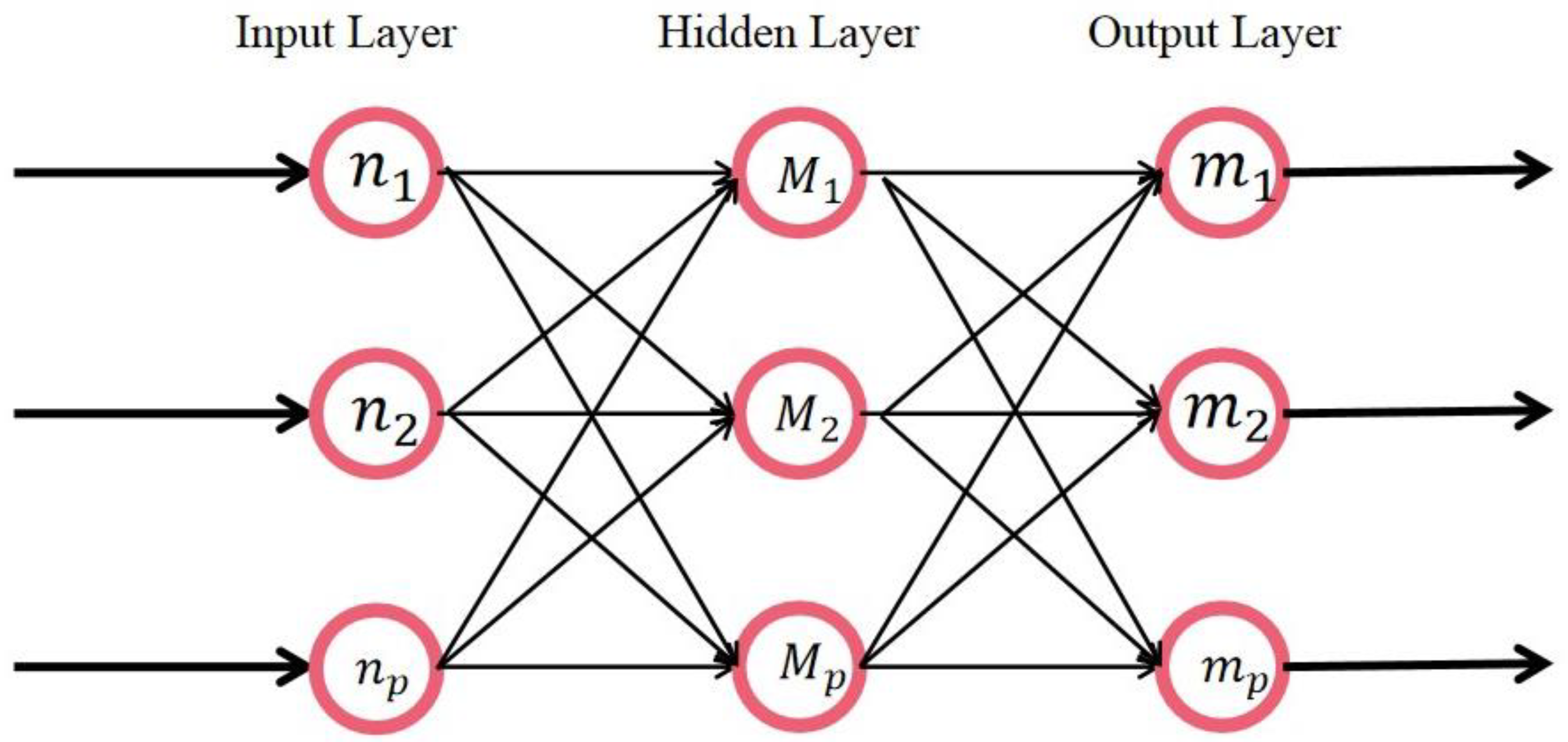
3.3. Principle on BP_NN

Back Propagation is the multilayer feed-forward NN, which is trained according to the error. It has the broadest applications among NN at present. BP-NN is typical of the forward network and has more than three layers without feedback. There is no interconnection within layers. Its structure is shown in Figure 3. The structure shows that the BP-NN neural network can realize the mapping from an n-dimensional input matrix to an m-dimensional output matrix by connecting the updated weight and threshold. In general, BP_NN uses the Sigmoid function or linear function as the transfer function.
f ( x ) = 1 1 + e x
In the BP_NN model, the node number of the hidden layer has a great influence on diagnostic accuracy. A smaller number of nodes reduces the ability of the net to learn, which required an increase in the number of training cycles. Too many nodes makes the training time longer, meaning that overfitting can easily occur. Reference [23] points out that the optimal number of hidden layer nodes must exist. For the exploration of this number of nodes, many scholars have given various solutions [24,25,26], including the use of the experimental method, the introduction of the hyperplane, dynamic full parameter self-adjustment and so on. A series of empirical formulas are obtained. After the summary, the optimal number of hidden layer nodes can be obtained. Refer to the following formula [24,25,26]:
l < m + n + a l = log 2 n
Here, the parameter n is the number of nodes on the input level, the variable l is the number of nodes on the intermediate level, the variable m is the number of nodes on the output level and the variable a is a constant between 0 and 10. In the paper, the input nodes (n) equal 8, the output nodes (m) equal 4 and the nodes of intermediate level are set to be 3.

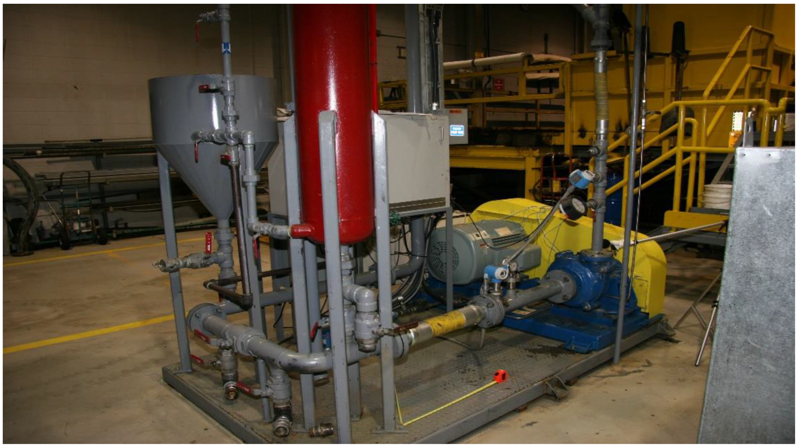
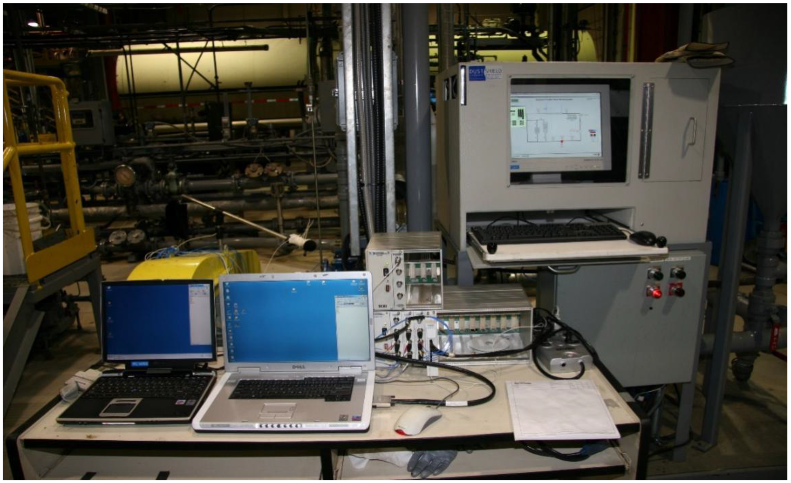
4. Experimental System of Centrifugal Pump

The industrial experimental system of the slurry pump is shown in Figure 4. The model for the centrifugal pump in the experiment is Weir/Warman 3/2 CAH with a closed impeller that is C2147. The diameter of the impeller is 8.5 inches. The centrifugal pump is driven by the motor. There is a V-belt drive between the motor and the centrifugal pump with a transmission ratio of 13/6. The parameters of the motor are shown in Table 1.
The vibration signal acquisition system is shown in Figure 5, which mainly consists of a signal analyzer and a laptop computer for storing data. The system acquires multiple channel signals including 3-axis vibration, acoustics, flow, pressure and temperature. The following conditions are satisfied for the acquisition of the experimental data.
(1)
Data collection does not begin until the centrifugal pump is running smoothly.
(2)
The sampling frequency satisfies the sampling theorem.
(3)
Multiple sets of data are collected for experiments conducted in each state.
In order to collect nonlinear multi-fault-mode characteristic signals, when the centrifugal pump is running steadily, the motor speed is set to be 1200 rpm for data acquisition. The data acquisition time of each group is 20 s. The sampling frequency is 9 kHz. The system synchronously collects online data on the vibration, acoustics, flow, pressure, etc. The nonlinear operation state of the machinery during the industrial process is simulated by controlling the flow rate and pressure of flow during the processing circuit, which consists of the nonlinear and nonstationary multi-failure mode.

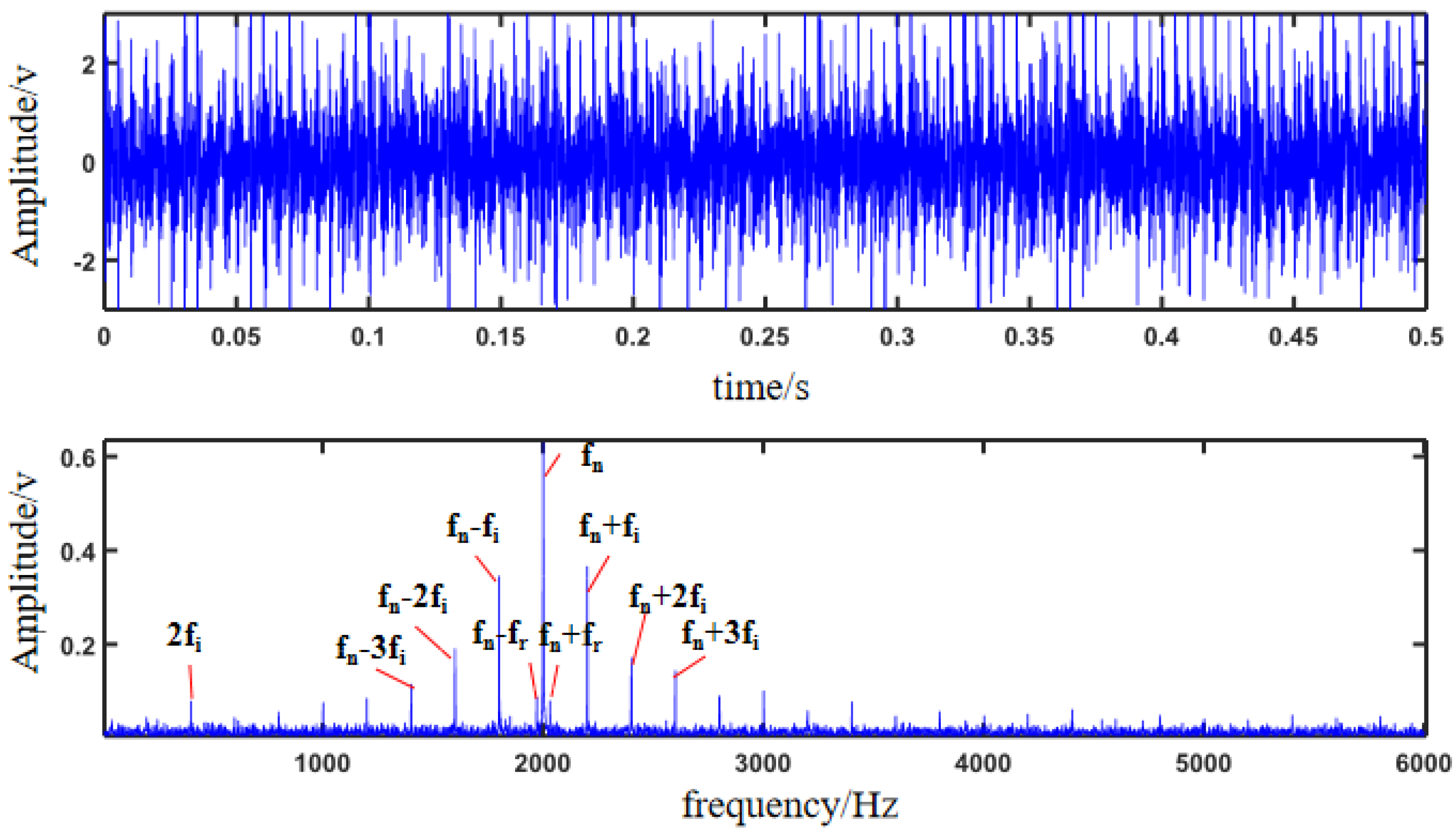
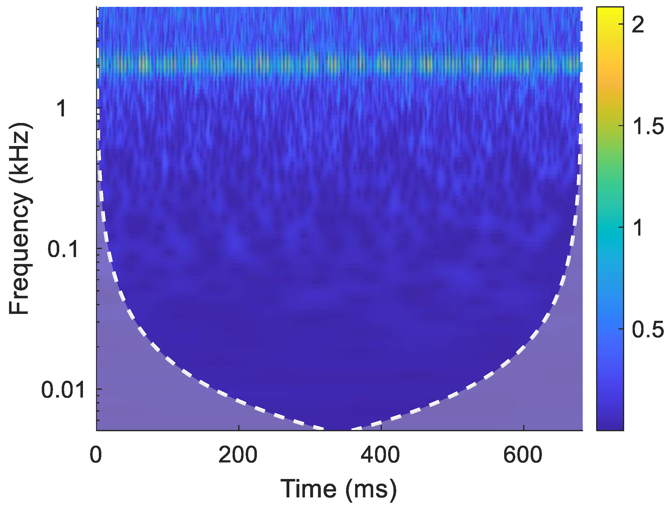
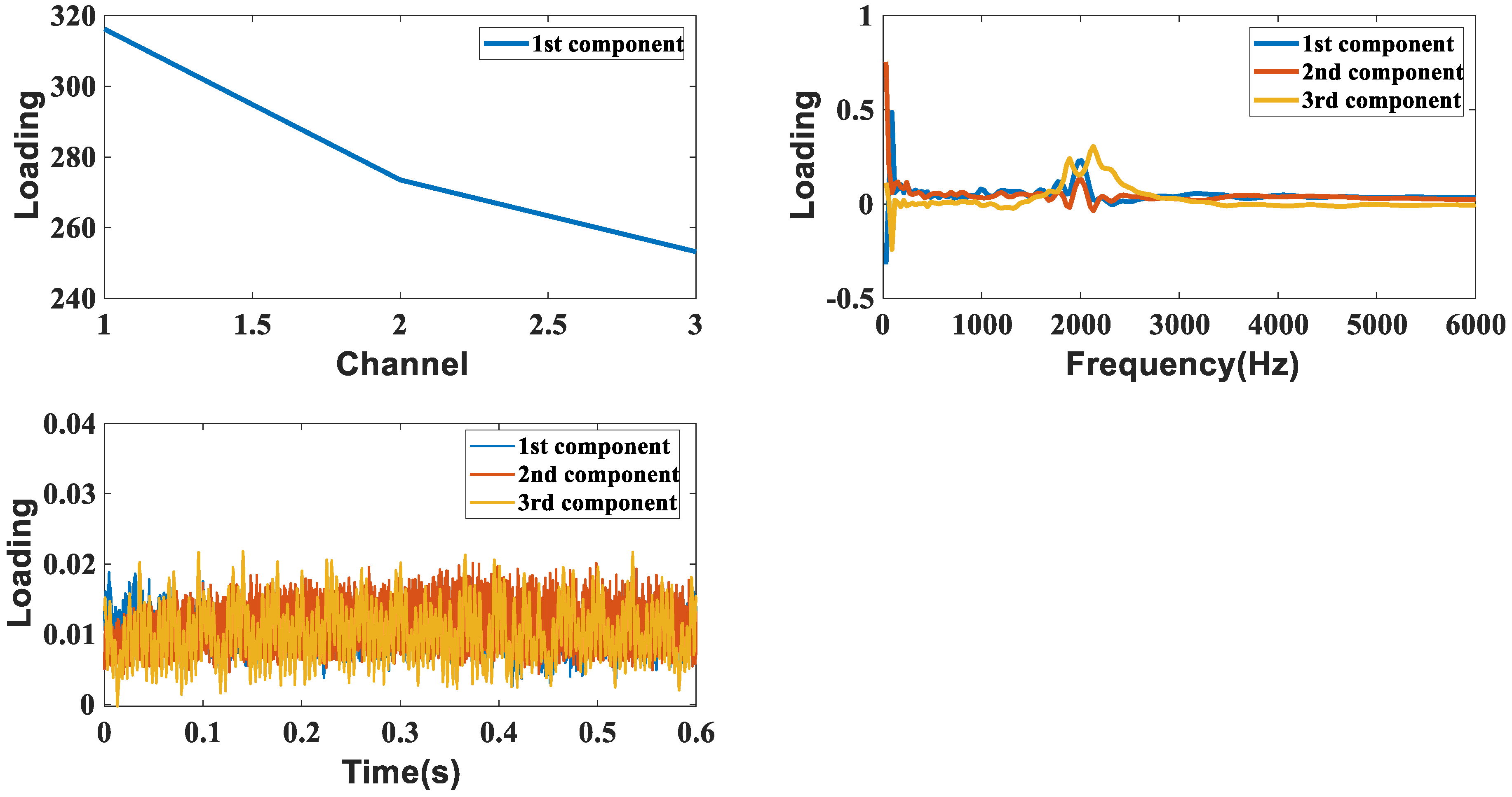
5. Simulated Signal for PARAFAC Analysis

Considering that the vibration signals acquired in the condition monitoring of mechanical equipment in the practical industrial environment generally were corrupted by the heavy noise signals, the typical numerical signal is generated to simulate the characteristic vibration information in the fault diagnosis of a mechanical system by using Equation (31), which is used to assess the effectiveness of the proposed method based on PAFARAF and continuous wavelet transform (CWT). The simulated signal consists of impulse signals when the fault occurs in the equipment and Gaussian White Noise (GWN) with 1 dB signal-to-noise ratio (SNR).
{ x ( t ) = s ( t ) + n ( t ) s ( t ) = i ( 1 + 0.2 cos ( 2 p i f r t ) ) e 700 ( t i / f i ) cos ( 2 p i f n ( t i / f i ) )
Here, the function s ( t ) is the periodic shock signal, the symbols f r and f i are the rotation frequency and faulty frequency, which are 30 Hz and 200 Hz. The inherent frequency f n is 2000 Hz. The symbol n ( t ) denotes the noise signal. The faulty signal is simulated to consist of the rotational frequency, faulty frequency and intrinsic frequency with noise corruption. The sampling frequency and analysis points are set as follows: f s = 12,000 , N = 8192 . The time and frequency domains of the simulated signal are shown in Figure 6, and it can be found that the fault characteristics are correlated with both the inherent frequency of the system and the rotation frequency of the motor shaft. It can be seen that the frequency components related to the fault characteristics include harmonic frequencies 2 f i , modulation frequencies f n n f i , and other frequencies. The key point for accurate fault identification is to extract the useful frequencies related to the faulty characteristics from the original noise signal.
Although the frequency domain of the simulated signal in Figure 6 presents the frequency information related to the fault characteristics, it is buried by heavy noise and inherent frequency-related components. The failure characteristics are buried and located in heavy noise. It is necessary for the corrupted data to be processed to extract the fault characteristic frequencies accurately. CWT is used to analyze the simulated impulse signal. The wavelet basis function is “comr3−3”. The center frequency of the wavelet function is 3 Hz. Figure 7 shows the CWT of the simulated signal. However, the fault-related frequency components are not filtered out, which indicates that the traditional time-frequency transformation is not effective enough to extract the weak fault characteristics of the frequency components from the simulated complex noised signal.
PARAFAC is a tensor decomposition algorithm and the decomposition is unique. In the case that the tensor models the N-dimensional relationship well, the parallel factor decomposition retains the original characteristic signal to a large extent while the feature caused by the failure component of the mechanical system is extracted effectively from the original complex system information. Based on the advantage of PARAFAC, the wavelet coefficients of the simulated signal after continuous wavelet transform are obtained, which is applied to construct one 3rd-order tensor with the dimension 1 × 200 × 8192. The tensor is decomposed by the parallel factor analysis to extract multiple factor components, which contain the channel, time and frequency information of the high-dimensional original signal. To build a correct parallel factor model, it is necessary to select the appropriate factor group fraction. The simulated signal determines the factor number F by considering the cross-validation and the kernel consistency method proposed in Section 3.
Figure 8 shows the cross-validation of the simulated signal. When the number of factors F is set to be from 1 to 3, the parallel factor cross-validation of the simulation signal is better in both the fitting group and the validation group. The values of the explanatory variables reach more than 80% and the kernel consistency of the parallel factor model reaches 100%. In summary, it is considered that the number of factors F is chosen as 3 to establish the parallel factor model for the tensor, which is constructed by the simulation signal for the data analysis.
Figure 9 shows the three subspaces which are obtained after the parallel factor decomposition of the simulated fault signal with noise addition. The loading values correspond to the channel, time and frequency information of the original signal. The residual values of the model fitting are obtained. The simulated signal is decomposed by PARAFAC into a frequency matrix, time matrix and time–frequency information. The amplitudes corresponding to the simulated impulse signal in the frequency matrix have obvious peaks at frequencies of 2000 Hz and 0~100 Hz, which shows the disadvantage that the low-frequency characteristics associated with the fault component are not clearly extracted. The time–information matrix obtained after the decomposition of the parallel factor is analyzed with the power spectrogram as shown in Figure 10. The comparison between Figure 7 and the results in Figure 9 and Figure 10 verifies that the PARAFAC algorithm has a great advantage in a more accurate and efficient form of feature extraction of the complex corrupted vibration signals in fault diagnosis as compared to the traditional time–frequency domain signal processing methods.

6. Discussion

Based on the simulated signal analysis as shown in Figure 9 and Figure 10, it has been verified that the time and frequency feature matrices can accurately characterize the fault model information. The multiple dimensional data model can be constructed by containing the acquired data from the accelerometer, flow sensor and pressure sensor, which is analyzed and processed by the PARAFAC algorithm. The time and frequency loading matrices are extracted as the characteristic signals. The forty sets of data are collected from the centrifugal pump system under one of the four running states that are normal (F1), impeller blade damage (F2), impeller edge damage (F3) and impeller perforation damage (F4), which are used to analyze the operation status of the centrifugal pump for the nonlinear multiple fault diagnosis.
Based on Nyquist’s sampling theorem, the maximum frequency of the signal spectrum is half of the sample frequency of 4500 Hz. The time for data acquisition in each mode of the impeller in the experiment is 20 s with eighteen thousand data points. A reduction in the complexity of data processing for a better comparison is required, and the proposed PARAFAC algorithm as described in Section 3 is used directly to obtain data points for the four failure modes for feature extraction.
PARAFAC was used to process the test data. We considered the vibration signals, flow signals and pressure signals from the multiple measurement points collected in the above experimental system for a total of the fifteen channel signals. The purpose of choosing 15 data channels is that the 15 physical system variables are sufficient as systematic characteristics to control the nonstationary operation status. The operating status of the centrifugal pump is evaluated comprehensively from the multiple physical information facets, which makes the fault diagnosis of the centrifugal pump more reasonable and effective.
The number of factors of the PARAFAC model can be determined by choosing the kernel consistent diagnosis method in Section 3. The number of factors ranges from 1 to 8. There are three groups of data to test the factors. Figure 10 shows nuclear consistency estimation.
As shown in Figure 11, when the number of factors is from 1 to 5, the kernel consistency values are above 60%. When the number of factors is greater than 5, the kernel consistency values decrease rapidly by 60%. Therefore, the amount of factors in the PARFAC model is chosen to be 5. The PARAFAC algorithm is solved by the trilinear alternating least squares method. Figure 12 shows the signal analysis by PARAFAC used to obtain the five components in mode 2 under four operating states when the angular speed is 1200 rpm. Mode 2 provides the frequency information. Figure 13 shows the signal analysis by PARAFAC used to obtain the five components in mode 3 under four operating states when the angular speed is 1200 rpm. Model 3 provides the time domain information.
The multi-channel complex signals are obtained from the centrifugal pump, which are analyzed by parallel factor decomposition to obtain the time and frequency information matrices. The time matrices as shown in Figure 13 are analyzed by Discrete Fourier Transform (DFT) to obtain the frequency domain information. DFT is defined as follows:
S ( k ) = N 1 k = 0 x ( k Δ t z ) e 2 π j n k N , ( n = 1 , 2 , , N 1 )
Figure 14 shows the spectra frequency of the fourth component under F1 and F2. The characteristic frequency under F2 is 250 Hz. Figure 15 shows the spectra frequency of the fifth component under F1 and F3. The characteristic frequency under F3 is 184 Hz. Figure 16 shows the spectra frequency of the third component under F1 and F4. The characteristic frequency under F4 is 20 Hz. The rotation speed of the motor in this experiment was set to 1200 rpm and the rotation frequency was 20 Hz. It is known that the fault characteristic frequency of the centrifugal pump impeller is generally related to the frequency component of the rotation frequency. The frequency of the impeller blade failure is expressed by the blade passing frequency, which is calculated by multiplying the rotation frequency by the number of blades, which was 20 × 10 = 200 Hz in this paper. Regarding the blade damage and impeller edge damage mode, the characteristic frequency is approximately distributed around 200 Hz. The characteristic frequency of the impeller perforation damage is 12 Hz, which is about 1/2 of the rotation frequency. Based on the above analysis, it has been verified that the parallel factor algorithm is more effective for the characteristic processing of the centrifugal pump multidimensional signal.
The time–frequency features extracted from the multi-source signals by PARAFAC decomposition are inputted to the BP model as features. The classification accuracy of the model was calculated. The output of the BP model and the corresponding state of the centrifugal pump are shown in Table 2.
The eight statistics of each component constitute the feature vectors for subsequent NP_NN and GA_BP_NN classification. The time and frequency domain statistics of each component are calculated as follows:
(1) Center of gravity frequency:
F 1 = k = 1 K f s S ( k ) k = 1 K S ( k )
(2) Root Mean Square (RMS) of spectrum
F 2 = 1 K 1 k = 1 K [ S ( k ) 1 K k = 1 K S ( k ) ] 2
(3) Frequency of root mean square (RMS)
F 3 = k = 1 K f k 2 S ( k ) k = 1 k S ( k )
(4) Peak Factor
P F = max | x ( i ) | 1 N i = 1 N x ( i ) 2
Clearance Factor
C L F = max | x ( i ) | ( 1 N i = 1 N | x ( i ) | ) 2
Waveform Factor
W F = 1 N i = 1 N x i 2 1 N i = 1 N | x ( i ) |
Impulse Factor
I F = max | x ( i ) | 1 N i = 1 N | x ( i ) |
Kurtosis Factor
K F = i = 1 N ( x ( i ) x ¯ ) 4 N ( i = 1 N ( x ( i ) x ¯ ) N ) 4 ( 1 N i = 1 N x i 2 ) 4
Figure 17 shows the diagnostic correction of centrifugal pump features in the BP_NN classification model. There is one mistake between the actual value and predicted value for F1 and five mistakes between the actual value and predicted value for F2. We improved the identification correction accuracy of fault status, as GA was applied to optimize the weights and thresholds between each connection layer of the BP_NN model. Figure 18 shows the diagnostic correction of centrifugal pump features in the GA_BP_NN classification model. There is just one mistake between actual value and predicted value for F3, which is much better than that for BP_NN without GA optimization.

7. Conclusions

Aiming at resolving the multiple failure modes of the centrifugal pump impeller, an experimental system of a centrifugal pump was developed to collect multi-channel complex fault signals for its operation state. The continuous wavelet transform was applied to analyze the multi-channel signals to construct 3D tensors. The hybrid method of the multiple-dimensional-data fusion was proposed based on PARAFAC, BP_NN and GA. The multi-dimensional signal analysis of the complex systems accurately located the fault frequency range of the centrifugal pump. An improvement in the diagnostic accuracy was achieved. Due to the limitations of experimental conditions, this paper only investigated the accuracy of the single fault classification of multi-channel signals, while the failure modes of mechanical equipment in actual production would be more complex, which also provides direction for future research.

Author Contributions

Conceptualization, S.L.; methodology, H.C.; software, M.L.; validation, S.L.; formal analysis, S.L.; investigation, S.L., M.L.; resources, H.C.; data curation, M.L.; writing—original draft preparation, S.L.; writing—review and editing, S.L., H.C.; visualization, M.L.; supervision, H.C.; project administration, H.C.; funding acquisition, H.C. All authors have read and agreed to the published version of the manuscript.

Funding

The National Natural Science Foundation of China (Grant 51775390).

Informed Consent Statement

Informed consent was obtained from all subjects involved in the study.

Data Availability Statement

Not applicable.

Acknowledgments

The experimental data were obtained from Lab of Reliability at University of Alberta in Canada.

Conflicts of Interest

The authors declare no conflict of interest.

References

  1. Wu, B. A brief discussion on the fault diagnosis and inspection and testing of lifting machinery. China Equip. Eng. 2021, 153–154. [Google Scholar]
  2. Xia, X.; Lu, Y.; Su, Y.; Yang, J. Mechanical fault diagnosis of high-voltage circuit breaker based on phase space reconstruction and improved GSA-SVM. China Electr. Power 2021, 54, 169–176. [Google Scholar]
  3. Zhao, P. Research on Vibration Fault Diagnosis Method and System Implementation of Centrifugal Pump. Ph.D. Thesis, North China Electric Power University, Beijing, China, 2011. [Google Scholar]
  4. Tong, Z.M.; Xin, J.G.; Tong, S.G.; Yang, Z.-Q.; Zhao, J.-Y.; Mao, J.-H. Internal flow structure, fault detection, and performance optimization of centrifugal pumps. J. Zhejiang Univ. Sci. A 2020, 21, 85–117. [Google Scholar] [CrossRef]
  5. Castellanos Barrios, M.; Serpa, A.L.; Biazussi, J.L.; Verde, W.M.; Natachedo Socorro Dias Arrifano Sassim. Fault identification using a chain of decision trees in an electrical submersible pump operating in a liquid-gas flow. J. Pet. Sci. Eng. 2019, 184, 106490. [Google Scholar] [CrossRef]
  6. Chen, Y.; Yuan, J.; Luo, Y.; Zhang, W. Fault Prediction of Centrifugal Pump Based on Improved KNN. Shock. Vib. 2021, 2021, 7306131. [Google Scholar] [CrossRef]
  7. Bordoloi, D.J.; Tiwari, R. Identification of suction flow blockages and casing cavitations in centrifugal pumps by optimal support vector machine techniques. J. Braz. Soc. Mech. Sci. Eng. 2017, 39, 2957–2968. [Google Scholar] [CrossRef]
  8. Niu, C. Research on Wind Turbine Drive Chain Fault Diagnosis Based on Big Data and Artificial Intelligence. Ph.D. Thesis, Shanxi University, Taiyuan, China, 2019. [Google Scholar]
  9. Xiaoshuai, G. Research on Online Monitoring and Fault Diagnosis Method of Electric Motor and Centrifugal Pump Set. Ph.D. Thesis, Beijing University of Chemical Technology, Beijing, China, 2020. [Google Scholar]
  10. Taqvi, S.A.A.; Zabiri, H.; Tufa, L.D.; Uddin, F.; Fatima, S.A.; Maulud, A.S. A Review on Data-Driven Learning Approaches for Fault Detection and Diagnosis in Chemical Processes. ChemBioEng Rev. 2021, 8, 239–259. [Google Scholar] [CrossRef]
  11. Cui, C.; Lin, W.; Yang, Y.; Kuang, X.; Xiao, Y. A novel fault measure and early warning system for air compressor. Measurement 2019, 135, 593–605. [Google Scholar] [CrossRef]
  12. Yu, Y.; Li, W.; Sheng, D.; Chen, J. A novel sensor fault diagnosis method based on Modified Ensemble Empirical Mode Decomposition and Probabilistic Neural Network. Measurement 2015, 68, 328–336. [Google Scholar] [CrossRef]
  13. Favier, G.; de Almeida, A.L.F. Overview of constrained PARAFAC models. Eurasip J. Adv. Signal Process. 2014, 2014, 142. [Google Scholar] [CrossRef] [Green Version]
  14. Krushal, J.B. Three-way arrays: Rank and uniqueness of trilinear decompositions, with application to artithmetic complexity and statistics. Linear Algebra Its Appl. 1997, 18, 95–138. [Google Scholar] [CrossRef] [Green Version]
  15. Yang, C. Research on the Application of Parallel Factor Analysis in Blind Separation of Multiple Fault Sources. Ph.D. Thesis, Nanchang University of Aeronautics, Nanchang, China, 2018. [Google Scholar]
  16. Li, J.F.; Zhang, S.F. Joint angular and Doppler frequency estimation of dual-base MIMO radar based on quadratic linear decomposition. J. Aeronaut. 2012, 33, 1474–1482. [Google Scholar]
  17. Nion, D.; Sidiropoulos, N.D. A PARAFAC-based technique for detection and localization of multiple targets in a MIMO radar system. In Proceedings of the 2009 IEEE International Conference on Acoustics, Speech and Signal Processing, Taipei, Taiwan, 19–24 April 2009; pp. 2077–2080. [Google Scholar] [CrossRef]
  18. Weis, M.; Romer, F.; Haardt, M.; Jannek, D.; Husar, P. Multi-dimensional space-time-frequency component analysis of event related EEG data using closed-form PARAFAC. In Proceedings of the 2009 IEEE International Conference on Acoustics, Speech and Signal Processing, Taipei, Taiwan, 19–24 April 2009; pp. 349–352. [Google Scholar] [CrossRef]
  19. Yang, L.; Chen, H.; Ke, Y.; Huang, L.; Wang, Q.; Miao, Y.; Zeng, L. A novel time–frequency–space method with parallel factor theory for big data analysis in condition monitoring of complex system. Int. J. Adv. Robot. Syst. 2020, 17, 172988142091694. [Google Scholar] [CrossRef] [Green Version]
  20. Li, Y.; Yuan, H.; Yu, J.; Zhang, C.; Liu, K. A review on the application of genetic algorithm in optimization problems. Shandong Ind. Technol. 2019, 12, 242–243. [Google Scholar]
  21. Zhao, G.S.; Huang, D.L.; Zhao, X. Fault diagnosis of mining rolling bearings based on RCMDE and GA-SVM. Coal Technol. 2021, 40, 221–223. [Google Scholar]
  22. Ma, J.; Meng, L.; Xu, T.; Meng, X. Research on bearing fault diagnosis by genetic radial basis neural network based on FastICA. Mach. Tools Hydraul. 2021, 49, 188–192. [Google Scholar]
  23. Rastegar, R.; Hariri, A. A Step Forward in Studying the Compact Genetic Algorithm. Evol. Comput. 2006, 14, 277–289. [Google Scholar] [CrossRef] [PubMed] [Green Version]
  24. Xu, Y.; He, M. Improved artificial neural network based on intelligent optimization algorithm. Neural Netw. World 2018, 28, 345–360. [Google Scholar] [CrossRef] [Green Version]
  25. Lv, Y.; Liu, W.; Wang, Z.; Zhang, Z. WSN Localization Technology Based on Hybrid GA-PSO-BP Algorithm for Indoor Three-Dimensional Space. Wirel. Pers. Commun. 2020, 114, 167–184. [Google Scholar] [CrossRef]
  26. Han, X.; Wei, Z.; Zhang, B.; Li, Y.; Du, T.; Chen, H. Crop evapotranspiration prediction by considering dynamic change of crop coefficient and the precipitation effect in back-propagation neural network model. J. Hydrol. 2021, 596, 126104. [Google Scholar] [CrossRef]
Figure 1. Tensor.
Figure 1. Tensor.
Ijtpp 07 00019 g001
Figure 2. Procedure for Parallel Factor Decomposition.
Ijtpp 07 00019 g002
Figure 3. Structure of BP_NN.
Ijtpp 07 00019 g003
Figure 4. Centrifugal pump experimental system.
Ijtpp 07 00019 g004
Figure 5. Data acquisition system.
Ijtpp 07 00019 g005
Figure 6. Corrupted simulation signal with noise.
Ijtpp 07 00019 g006
Figure 7. Wavelet transform of the simulated signal.
Ijtpp 07 00019 g007
Figure 8. Cross-validation for simulated signal.
Ijtpp 07 00019 g008
Figure 9. Parallel factor decomposition of simulated signal.
Ijtpp 07 00019 g009
Figure 10. Power spectrum of decomposed time domain loading matrix with PARAFAC.
Ijtpp 07 00019 g010
Figure 11. Nuclear consistency estimation.
Ijtpp 07 00019 g011
Figure 12. The 1200 rpm centrifugal pump signal decomposition in Mode 2: (F1) for normal impeller, (F2) for blade damage, (F3) for impeller edge damage, (F4) for impeller perforation damage.
Ijtpp 07 00019 g012
Figure 13. 1200 rpm centrifugal pump signal decomposition in Mode3: (F1) for normal impeller, (F2) for blade damage, (F3) for impeller edge damage, (F4) for impeller perforation damage.
Ijtpp 07 00019 g013
Figure 14. Spectra analysis of fourth component under F1 and F2.
Ijtpp 07 00019 g014
Figure 15. Spectra analysis of fifth component under F1 and F3.
Ijtpp 07 00019 g015
Figure 16. Spectra analysis of third component under F1 and F4.
Ijtpp 07 00019 g016
Figure 17. Comparison between the actual and predicted values by BP_NN.
Ijtpp 07 00019 g017
Figure 18. Comparison between the actual and predicted values by GA_BP_NN.
Ijtpp 07 00019 g018
Table 1. Motor parameters.
ModelRated
Voltage (V)
Maximum Speed (RPM)Rated Speed (RPM)Rated
Ambient Temperature (°C)
Rated Power (HP)Overload FactorMotor Size
230/4601200118040401.15362 T
Table 2. Expected output of neural network corresponding to each state of centrifugal pump.
Output Label1234
F11000
F20100
F30010
F40001
Publisher’s Note: MDPI stays neutral with regard to jurisdictional claims in published maps and institutional affiliations.

