A Self-Learning Fault Diagnosis Strategy Based on Multi-Model Fusion


1
Logistics Engineering College, Shanghai Maritime University, Shanghai 201306, China
2
Institut de Recherche Dupuy de Lôme UMR CNRS 6026 IRDL, University of Brest, Brest 29238, France
3
Group of Electrical Engineering Paris UMR CNRS 8507, CentraleSupelec, Univ. Paris Sud, Sorbonne Université, Gif-sur-Yvette 91192, France
*
Author to whom correspondence should be addressed.
Information 2019, 10(3), 116; https://0-doi-org.brum.beds.ac.uk/10.3390/info10030116
Submission received: 11 January 2019
/
Revised: 12 March 2019
/
Accepted: 13 March 2019
/
Published: 17 March 2019
(This article belongs to the Special Issue Fault Diagnosis, Maintenance and Reliability)
Abstract
:This paper presents an approach to detect and classify the faults in complex systems with small amounts of available data history. The methodology is based on the model fusion for fault detection and classification. Moreover, the database is enriched with additional samples if they are correctly classified. For the fault detection, the kernel principal component analysis (KPCA), kernel independent component analysis (KICA) and support vector domain description (SVDD) were used and combined with a fusion operator. For the classification, extreme learning machine (ELM) was used with different activation functions combined with an average fusion function. The performance of the methodology was evaluated with a set of experimental vibration data collected from a test-to-failure bearing test rig. The results show the effectiveness of the proposed approach compared to conventional methods. The fault detection was achieved with a false alarm rate of 2.29% and a null missing alarm rate. The data is also successfully classified with a rate of 99.17%.
1. Introduction
Because of higher requirements in terms of effectiveness and economic performances, modern industrial systems have become more complex [1]. The increasing number of components and the complex operating modes increase the failure rate [2,3,4]. Therefore, in order to respect the safety and reliability requirements, fault detection and diagnosis strategy should be implemented to monitor the system. The current fault diagnosis approaches can be broadly separated into physics-based and data-driven ones [3,4,5]. Due to the complexity of the modern industrial system, it is difficult to establish an accurate analytical model based on physics [6]. Besides, most of the processes are increasingly controlled with computers. Therefore, a huge amount of data is available, making data-driven methods very attractive [7].
Multivariate statistical analysis and machine learning are becoming more and more popular as feature extraction and analysis tools for fault diagnosis using a data-driven approach [8]. Among the statistical analysis methods, the Principal Component Analysis (PCA) has been widely used in process monitoring [9,10,11,12,13]. However, PCA is optimal when the data follows a Gaussian distribution [14]. Therefore, Z. Q. Ge has presented a PCA-1-support vector machine (SVM) model and Y. Zhang et al. applied an Independent Component Analysis (ICA) for fault detection [15,16]. However, when the distribution is more complex the usual fault detection methods have lower performances. Thus, L. R. Arnaut et al. proposed different combinations of the ICA and PCA [17,18] to the detriment of a higher computational burden. Moreover, the behaviors in real industrial processes are usually nonlinear [19,20]. Therefore, important information can be lost with poor fault detection performances when using linear transformations [21]. To address this issue, B. Schölkopf et al. proposed the kernel method [22], such as the Kernel Principal Component Analysis (KPCA) and the Kernel Independent Component Analysis (KICA) [23,24,25,26]. However, the assumption of independent and identically distributed variables should stand [27,28,29,30,31]. Some machine learning methods such as the Extreme Learning Lachine (ELM) and Support Vector Machine (SVM) have good performances with a nonlinear process, with no assumptions on the variables. However, ELM often requires a large amount of label data for off-line training, which are not always available in real industrial processes [27]. Thus, V. Vapnik et al. proposed the Support Vector Machine (SVM) to address the classification of small sample data [32]. SVM is another application of the kernel method, which has better generalization performance and nonlinear processing capability [33]. Despite that it can extract nonlinear features and effectively detect the faults, it requires a lot of time in the training stage and testing stage. Therefore, Tax et al. proposed the soft margin Support Vector Domain Description (SVDD) [34].
Moreover, in addition to nonlinear characteristics, the actual industrial processes have different steady-state and transient operating points. Therefore, it is difficult to achieve accurate monitoring with only one model that cannot cope with all the dynamics [35]. All the above-mentioned methods are based on one model. Therefore some academics have evaluated new techniques such as relative PCA (RPCA), Online Sequential ELM (OS-ELM), dynamic ICA and dynamic HyperSphere SVM (HSSVM). There were some improvements but not for all the operating modes.
In this paper, we propose an approach based on multi-model fusion to take into account all the operating points. We propose also to combine different techniques for fault detection and classification. Moreover, to enlarge the initial database, all the new samples well classified in both the fault detection and the fault classification steps are included in the database; this is known as self-learning. To evaluate our approach, real bearing data from the Center for Intelligent Maintenance Systems (IMS), University of Cincinnati is used [36]. The paper is organized as follows: The fault diagnosis strategy is introduced in Section 2. Section 3 describes a specific case for fault diagnosis in complex conditions. Section 4 introduces the experimental bearing data set and the fault detection and classification results. Finally, conclusions are drawn in Section 5.
2. Fault Diagnosis Method
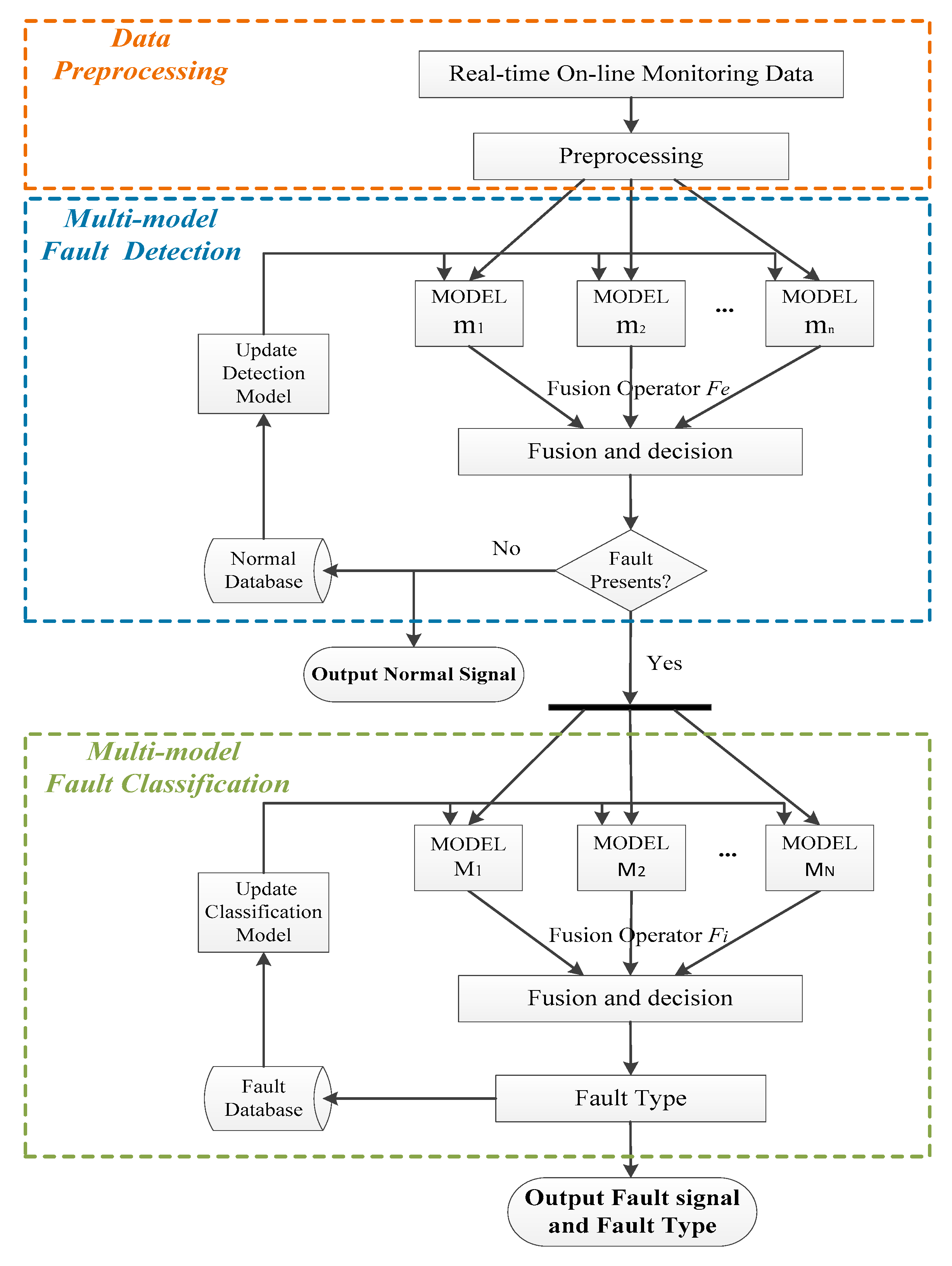
In this section, the fault diagnosis strategy is proposed. We use a small amount of normal and faulty operation data to establish several detection and classification models. The overall architecture of the proposed diagnosis strategy is illustrated in Figure 1. The method is based on three different modules namely pre-processing, fault detection and fault classification. The detailed content of each module is described in the following:
➢ Data Pre-Processing Module
During the offline step, historical healthy and faulty data are collected to train the detection models m1, m2, …, mn and the classification models M1, M2, …, MN.
➢ Fault Detection Module
In this module, the real-time data sample after pre-processing is fed through each detection model. Then, according to the results of each model, a fusion operator Fe is used to make a decision. If a fault is detected, the fault classification step is activated.
➢ Fault Classification Module
After a fault has been detected, the fault classification is started based on the classification models of M1, M2, …, MN. Then, according to the results of each model, a Fusion operator Fi is used to make a decision. Then according to the requirement of self-learning, if the results of the classification models meet the requirement of self-learning, it will use the real-time data sample to update them.
The following rules are specified when selecting the models for detection or classification:
2.1. Fault Detection
- ➢
- The detection models we choose are different from each other, or they can be complementary, in order to decrease false alarms and missing alarm rates.
- ➢
- The detection models need to have a high detection accuracy to avoid a cumulative error.
- ➢
- As the detection models will run in parallel, judicious implementation approaches can be used in combination with a multi-core and graphics processing unit (GPU)-based system to reduce the computational time.
2.2. Fault Classification
- ➢
- The classification models are different from each other, in order to increase the classification accuracy.
- ➢
- The classification models need to have a high classification accuracy to avoid the occurrence of cumulative error.
- ➢
- The computational time of each classification model must be as short as possible. Indeed, for fault classification, the time constraint is less.
Fusion is used to make the final decision from the output of the different models. Different methods can be used, such as voting, Bayesian inference and the behavior-knowledge space method. Bayesian inference requires more data and prior knowledge, and the behavior-knowledge space method needs a large storage space to record the identification results. For the sake of simplicity, we will use the voting method, which is described hereafter.
Each classifier model emits a vote (yi for classifier i) and the accumulated vote for each class is calculated as follows:
where wi is the weight value of the ith classifier and y is the result of the fusion.
In order to enrich the database, since it may not be large enough, a self-learning method is proposed. But before inserting the current sample in the database, the output of the diagnosis result must be consistent with the actual result. Therefore, we can avoid adding in the database erroneous prediction data.
3. Case of Complex Condition
In real systems, there are a lot of interactions and complex phenomenon that take place. They usually involve multi-physics and the behaviors are nonlinear, and the data distribution may be complex. As a consequence, one model cannot catch all the dynamics accurately. Therefore, in order to design an efficient online monitoring approach, different models are required for fault detection and classification.
3.1. Fault Detection
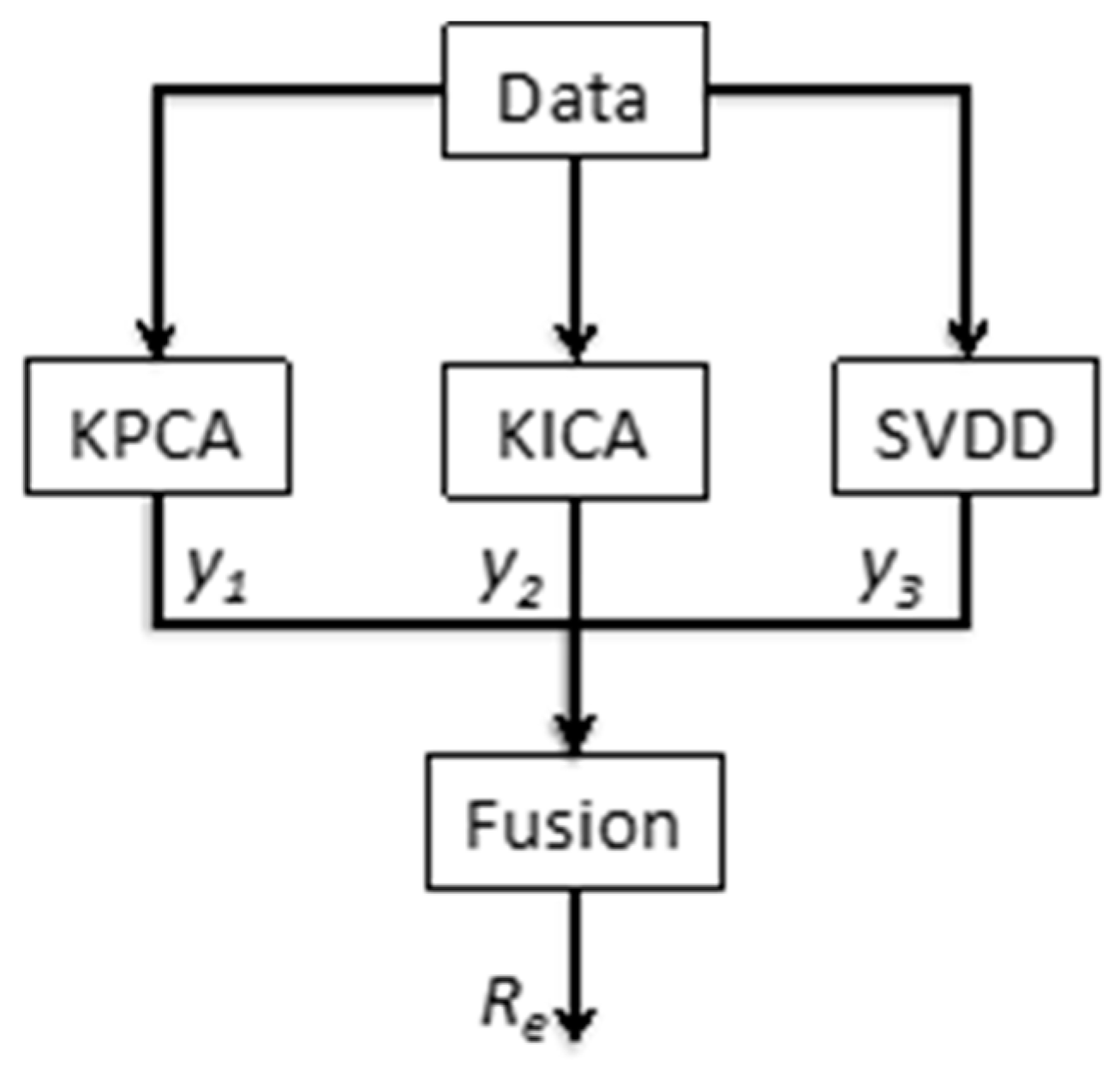
For fault detection, three models will be combined through a fusion operator. The first model is based on KPCA and the Hotelling T2 statistics [13,30]. The second one is based on the KICA [31] and the I2 statistic [33]. The third model uses the SVDD and the distance between the test sample, and the center of a hypersphere is used as the fault detection feature [27,34]. The flowchart is described in Figure 2.
The decision function for the KPCA is:
where Tcl2 is the confidence limit of T2 statistic. The details of this method can be found in Reference [13].
The decision function for the KICA is:
where Icl2 is the confidence limit of the I2 statistic. The details of this method can be found in Reference [34].
The decision function for the SVDD is:
The sample is faulty if yi = 1, (i = 1, 2, 3) or healthy if yi = -1, (i = 1, 2, 3). r is the radius of the high dimensional sphere and d is the distance from the detection point to the center of the high dimensional sphere.
We use a vector to express the results above, which is y = [y1, y2, y3], and the fusion operator is Fe = [ω1,ω2,ω3] where .
Because the KPCA is not optimal if the signal has a non-Gaussian distribution, we set its weight as a decreasing function. The same weight is adopted for the KICA for the same reason. Therefore, we set . While for the SVDD we use an increasing function for the weight to emphasize its contribution then . Where k = 0.1, s is the update times, and τ is a value of experience.
Then the decision result is:
If Re = 1, a fault is detected. If Re = 0 or −1, the sample is used to update the model(s) that have detected that no fault has occurred.
3.2. Fault Classification
For fault classification, a neural network (NN) based on single-hidden layer feedforward NNs (SLFNs), called the extreme learning algorithm (ELM) is used. To catch all the dynamics of the system, four different activation functions (hardlim, sin, radbas, and sigmoid) are used corresponding to three different models. Their outputs will be combined through a fusion operator that will be described in the following.
For the fusion step, an average weighting is used with the same weight ) for each of the four models as they have the same effect on the output. The fusion result is defined as:
where Fvote(x) is fault type of the final decision, gi(x) is the voting time of ith fault by these classification models and K is the number of fault types.
The self-learning fault diagnosis rule is as follows: When a fault is detected but all the four models cannot classify the fault type, the upcoming signal is stored and considered as data representing a new fault type.
4. Experimental Results and Analysis
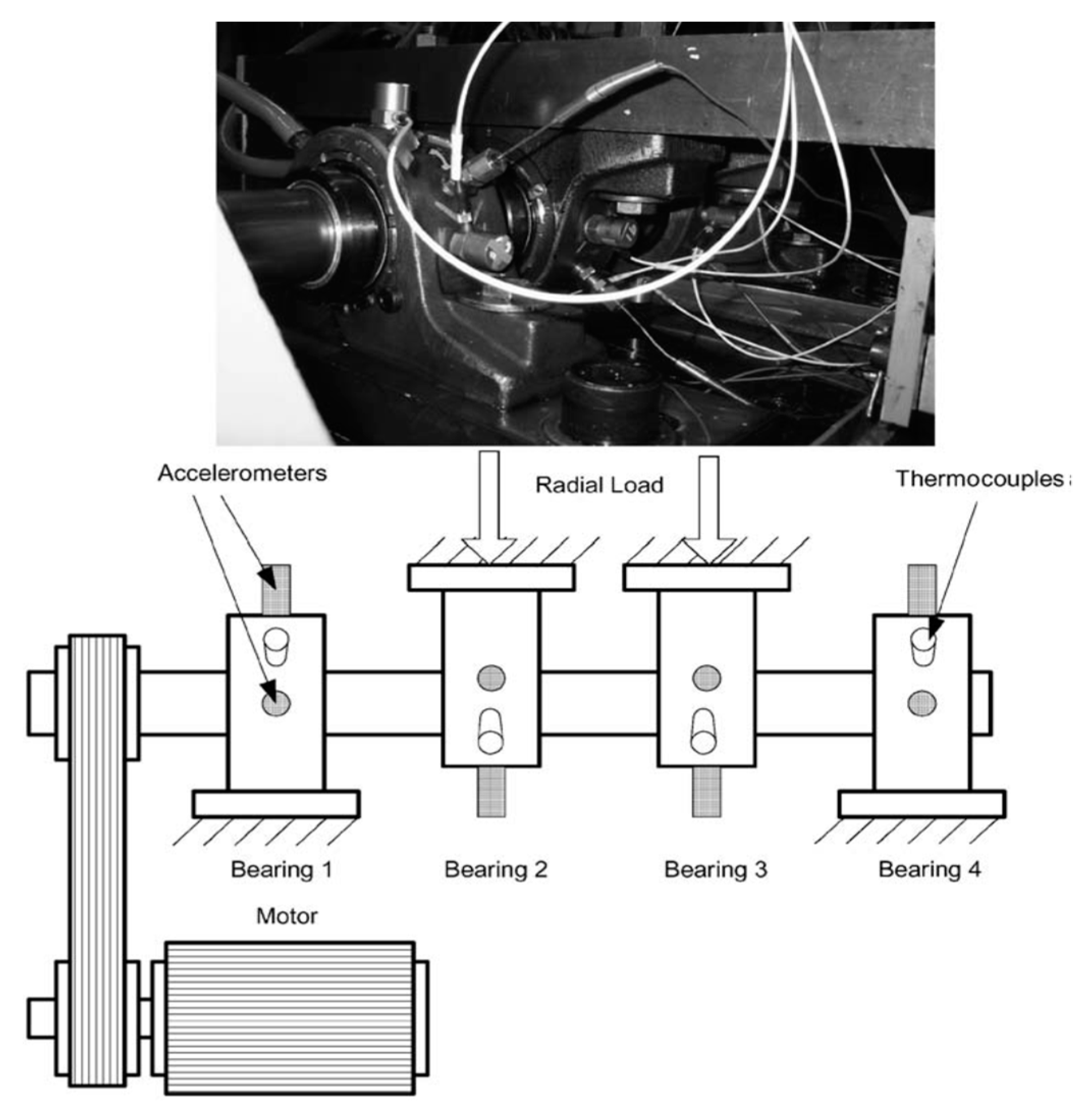
A data set of a real bearing test was chosen as the real-time input to test the proposed strategy. The bearing test data set was provided by the Center for Intelligent Maintenance Systems (IMS), University of Cincinnati [36]. The detailed bearing test rig and the schematic diagram of the installation are displayed in Figure 3 [37].
Four bearings were installed on a motor-driven shaft, and the rotation speed was set at 2000 rpm. A radial load of 6000 pounds was applied onto the shaft and the bearing by a spring mechanism. The data were collected with a NI DAQ Card 6062E, and the sampling rate was 20 kHz (each file contained 20,480 points). There were three data sets included in the data packet, and each data set consisted of a test-to-failure experiment. To evaluate the performance of the proposed approach, the data were organized in different sections, as described in Table 1, with the healthy data and three fault types.
4.1. Fault Detection
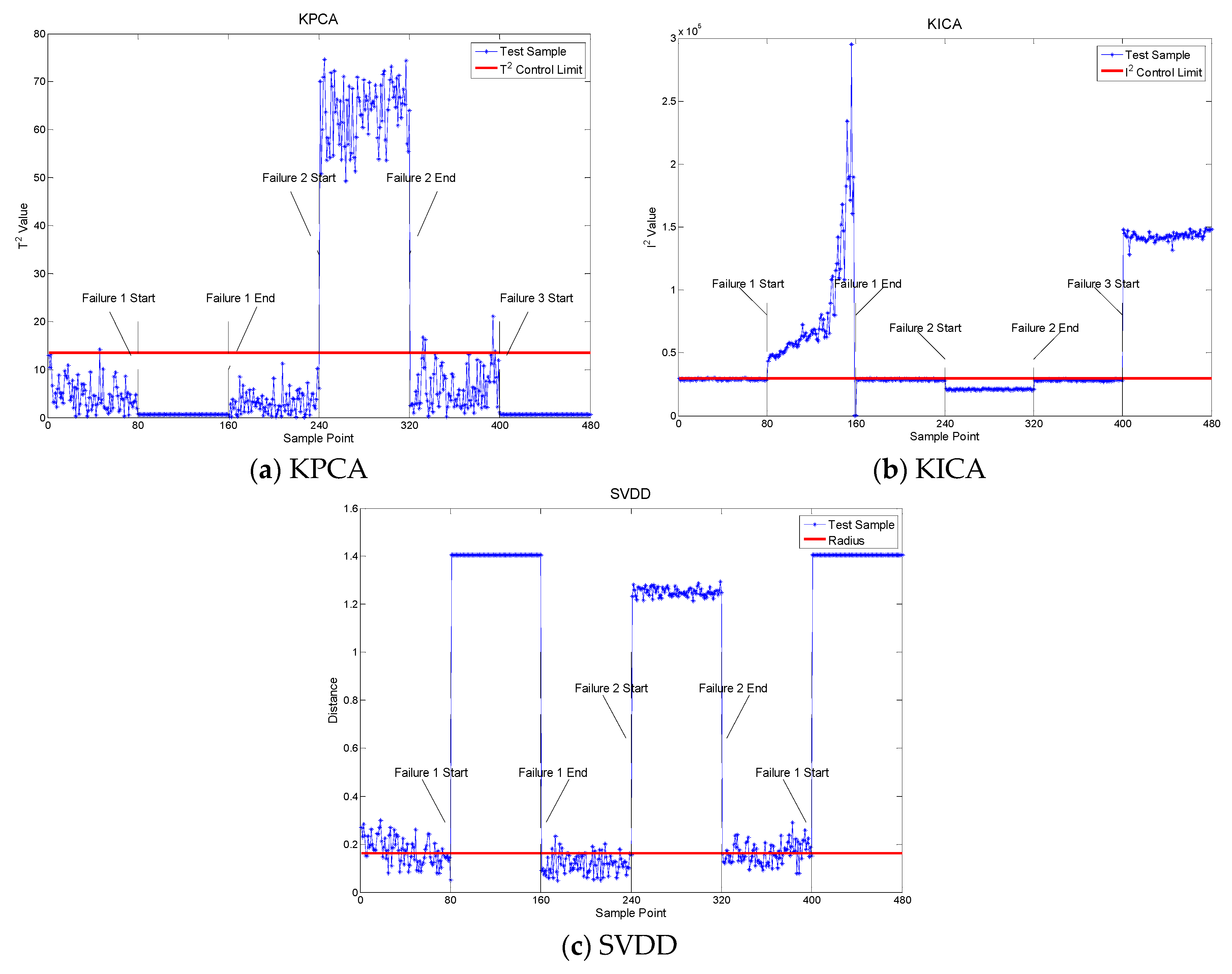
Figure 4 shows the fault detection result using the KPCA, KICA and SVDD. In Figure 4a, the red line is the confidence limit of the T2 statistic. The result showed that fault 2 can be detected with good performance. However, the KPCA failed to detect fault 1 and fault 3, and there were many false alarms. Moreover, the insufficient historical healthy sample also contributed to the poor fault detection results.
Figure 4b displays the fault detection result using the I2 statistic monitoring with the KICA. The results showed that fault 1 and fault 3 were clearly detected, while fault 2 was not detected. Figure 4c shows the fault detection result with the SVDD. The red line is the radius of the hypersphere obtained with the healthy data samples. Despite a high false alarm rate, the fault detection performances were fairly good.
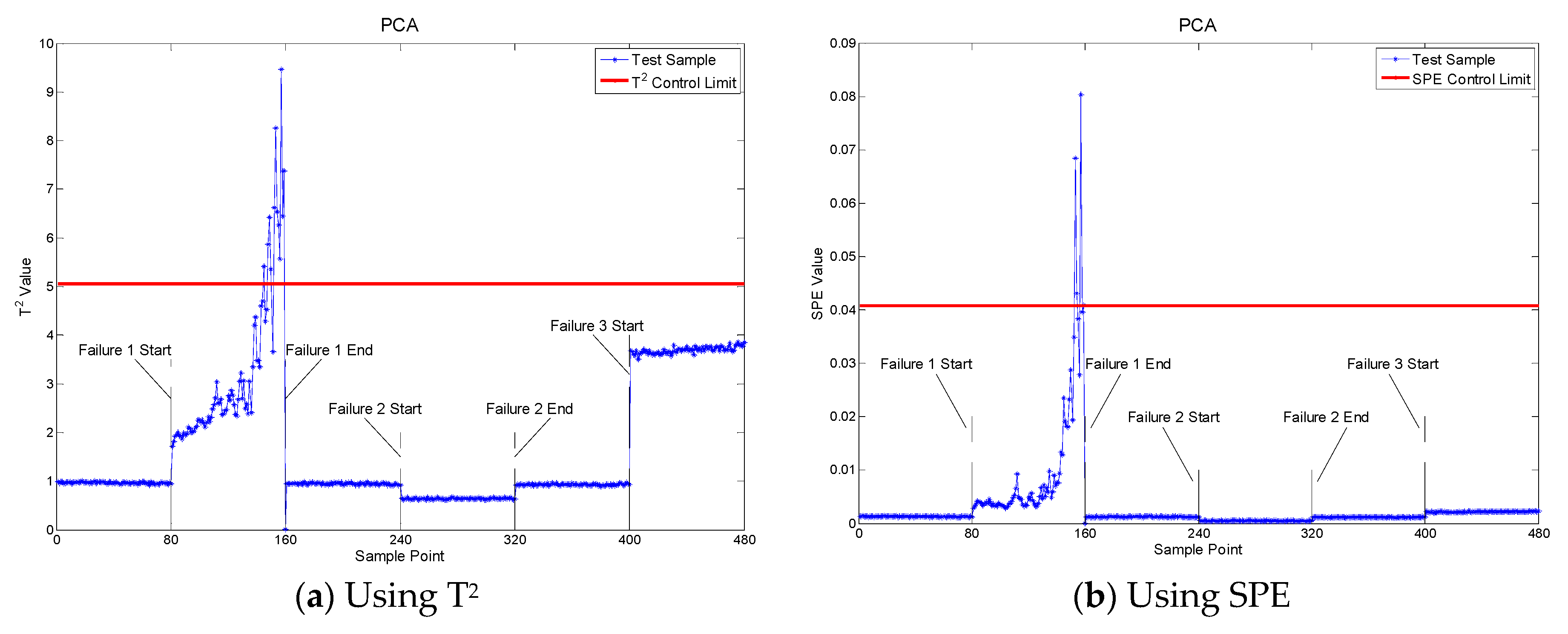
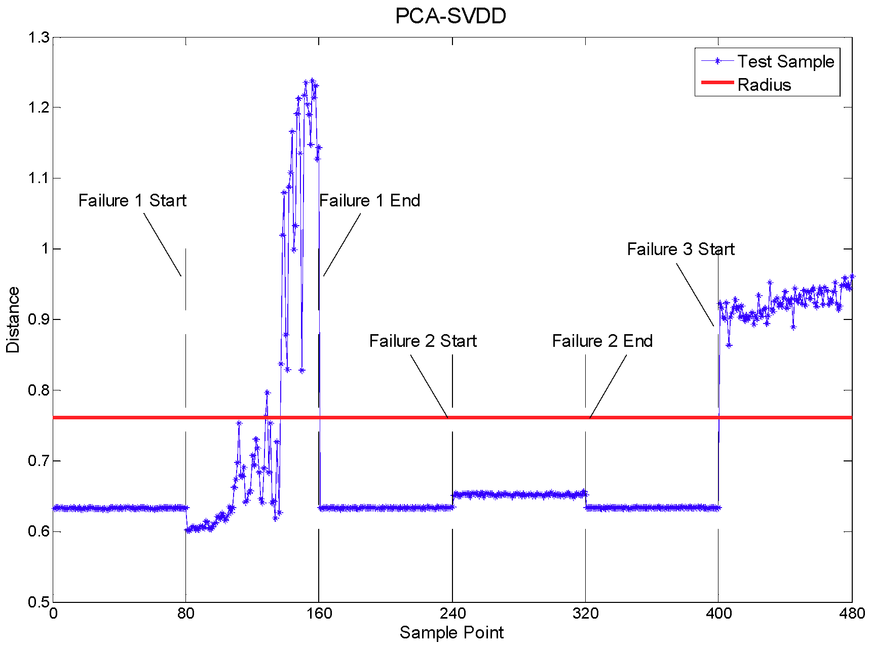
The PCA and PCA-SVDD were also evaluated with the same data. Figure 5 displays the fault detection result with two metrics: The Hotelling T2 and square predictive error (SPE) statistic, respectively. The performances were obviously very poor. Significant improvements were obtained when the SVDD was used to analyze the features extracted with the PCA. The results are plotted in Figure 6.
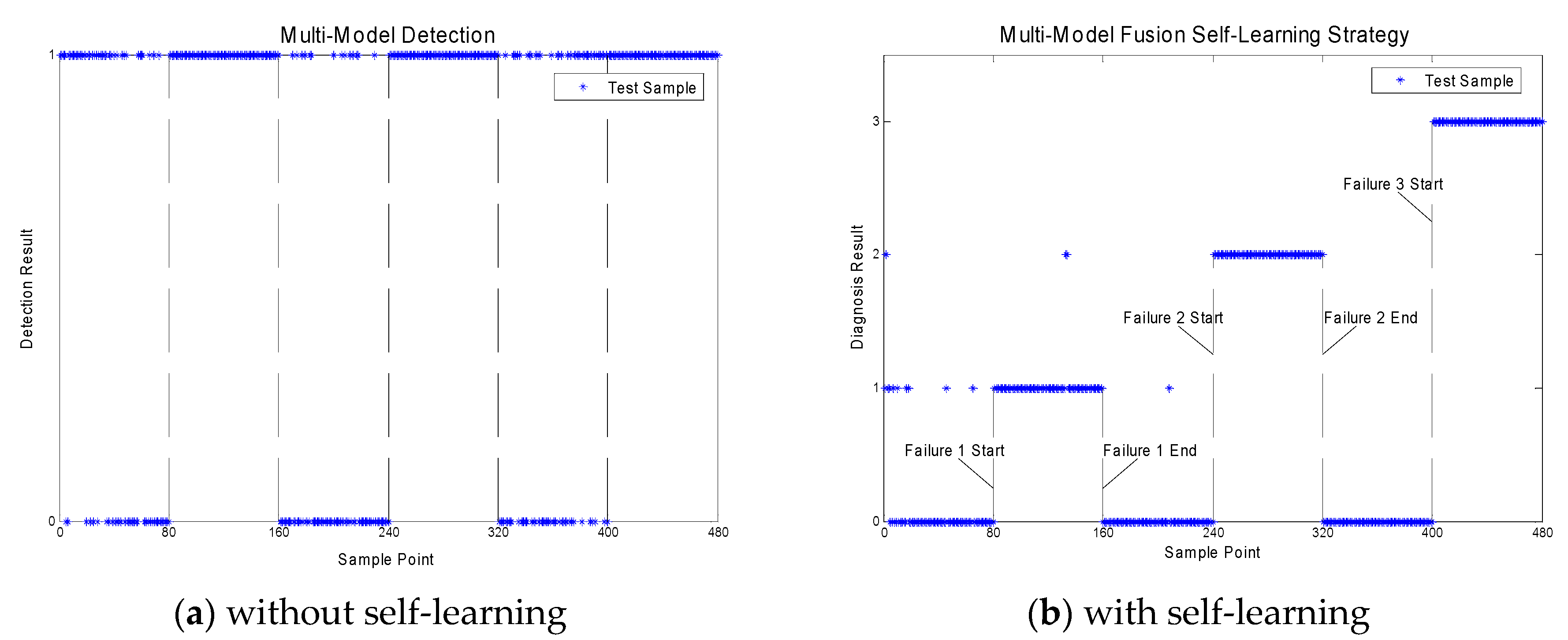
Finally, a multi-model strategy without self-learning was evaluated with the same data samples. The results plotted in Figure 7a showed a clear improvement of the fault detection for all three faults. However, this method suffered from a high false alarm rate. The self-learning was introduced with a fusion operator and the results are plotted in Figure 7b. All faulty samples were detected, and the data of fault 2 and fault 3 are all accurately classified. Furthermore, the classification accuracy of fault 1 reached 97.5%.
The fault detection results are summarized in Table 2 with the false alarm and missing alarm rates. The fusion of the models and the self-learning clearly exhibited higher performances. Its false alarm rate was far lower than 5%, which is a commonly adopted setting in industrial processes.
4.2. Fault Classification
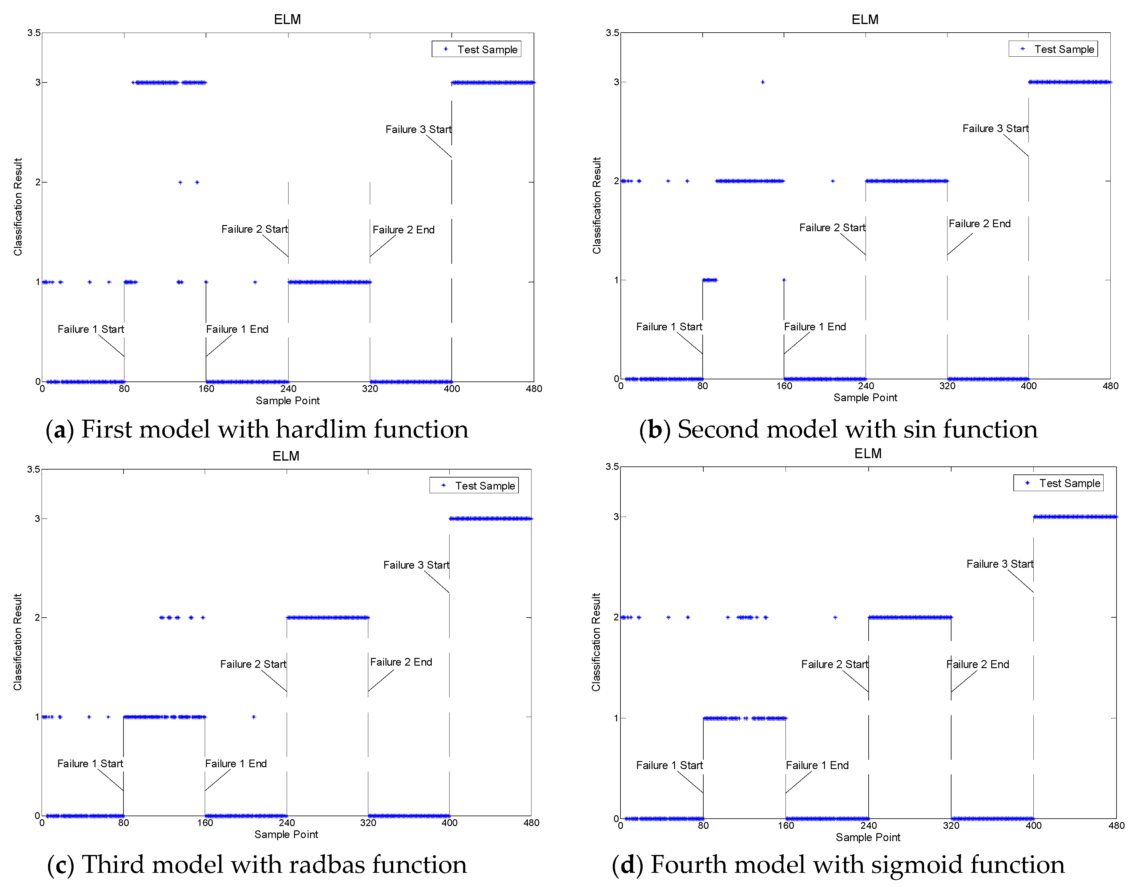
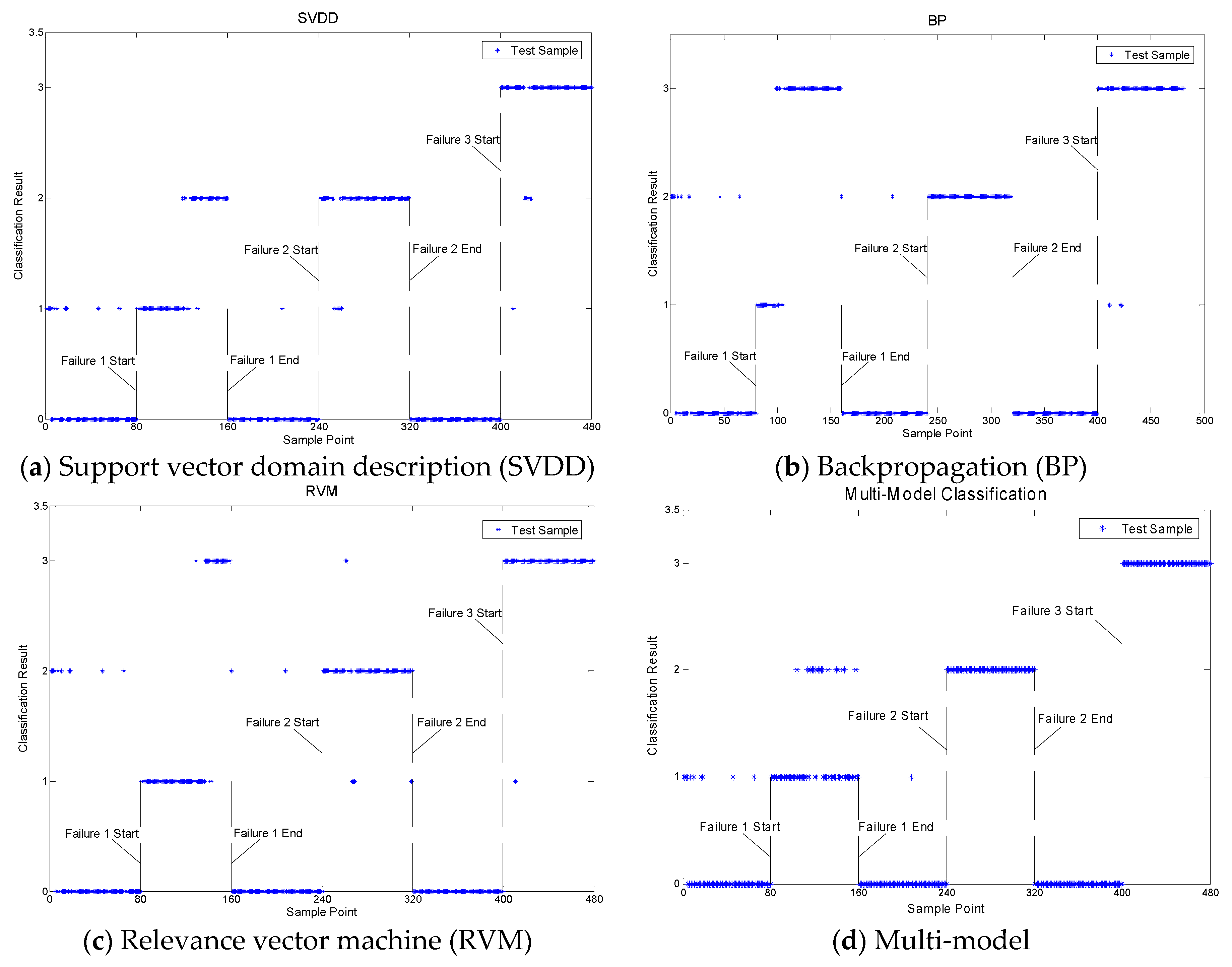
The ELM, SVDD, BackPropagation (BP) and Relevance Vector Machine (RVM) approaches were compared with the proposed strategy in the fault classification step. Figure 8 shows the classification result of the ELM. There were different layers for different faults. For example, some samples of fault 1 were classified in layer 1, which was correct. If the samples of fault 1 were classified in layers 2, 3 or 0, they were wrong. We used the four models to classify the faults respectively, since the different ELM models had different results in the fault classification. It can be seen that the classification results were not good. And the average accuracy of these four ELM models was used to express the classification accuracy of the ELM. The overall accuracy of the ELM was only 75.20%. The main reason was as follow: The historical sample was small, which meant that the model did not get enough training. We established the SVDD, which used these three different fault data in the classification phase, and the classification result of the SVDD, as shown in Figure 9a. The classification result was good for fault 2 and fault 3, but not good for fault 1. Figure 9b is the classification result of the BP model. The data of fault 2 were all classified correctly, but the overall classification accuracy was not ideal, being only 74.58%. BP needs a lot of time in the training phase, which made it difficult to achieve the online monitoring. Figure 9c depicts the classification result of the RVM. It had good classification accuracy in the data for faults 2 and 3. However, a lot of fault 1 samples were misclassified as fault 3. The overall accuracy of the RVM was higher than the ELM, BP, and SVDD. But the RVM is a binary classifier, which requires the establishment of a plurality of the RVM classifier, when used in multiple fault diagnoses. Therefore, it greatly increased the complexity of the calculations. The same as the detection phase, this paper also uses a multi-model strategy to illustrate the effect in the proposed strategy. Figure 9d shows the classification results with the multi-model. The overall classification accuracy was 92.5%. So the classification precision was improved with the multi-model compared with the single model approach. Table 3 shows the classification result of a comparison when the five approaches were used for fault classification of the bearing test for the same condition. Faults 1, 2, and 3 were well classified using the proposed strategy. In addition, its overall accuracy was higher than the single multi-model approach, which proved the positive effect of the self-learning.
The classification results are summarized in Table 3.
From the results displayed in Table 3, we could derive that the best detection and classification performance was achieved with the multi-model combined with the self-learning strategy.
5. Conclusions
In current industrial processes, competitiveness requires condition-based maintenance to reduce unwanted stops and maintenance costs. Health monitoring is one of the tools to reach these targets. However, the processes are more complex as they involve different physical phenomenon and highly nonlinear behaviors. The operating points are also variable. As a consequence, a single model would not be able to catch all the dynamics of the data for health monitoring. This paper has therefore proposed a fault diagnosis strategy based on multi-model and self-learning. In the fault detection step, the KPCA, KICA, and SVDD were used and combined with a fusion operator. In the classification step, the ELM was used with different activation functions combined with an average fusion function. This strategy was evaluated with bearing test-to-failure experiment vibration data. The fault detection was achieved with a false alarm rate of 2.29% and a null missing alarm rate. The data were also successfully classified with a rate of 99.17%. The proposed method can also be applied to other fields [38,39,40,41,42]. It should be mentioned that the proposed strategy could increase the computation time. Fortunately, processors are becoming more and more powerful and the software can be judiciously partitioned into several processors in a multicore system for real-time monitoring. The monitoring can also be engaged periodically if it is necessary to reduce the computational burden.
Author Contributions
T.W. proposed the multi-model fusion approach; J.D. and T.X. performed the simulations and the tests; T.W., D.D., and M.B. verified the simulation and test results and supervised the whole research procedure of this paper.
Funding
This research is supported by the National Natural Science Foundation of China (61673260) and the Shanghai Natural Science Foundation (16ZR1414300).
Conflicts of Interest
The authors declare no conflict of interest.
References
- Gao, Z.; Ding, S.; Cecati, C. Real-time fault diagnosis and fault-tolerant control. IEEE Trans. Ind. Electr. 2015, 62, 3752–3756. [Google Scholar] [CrossRef] [Green Version]
- Xu, X.; Li, S.; Shen, X.; Wen, C. The optimal design of industrial alarm systems based on evidence theory. Control Eng. Practice 2016, 46, 142–156. [Google Scholar] [CrossRef]
- Wen, C.; Wang, Z.; Hu, J.; Liu, Q.; Alsaadi, F. Recursive filtering for state-saturated systems with randomly occurring nonlinearities and missing measurements. Int. J. Robust Nonlinearity Control 2018, 28, 1715–1727. [Google Scholar] [CrossRef]
- Wang, T.; Liu, L.; Zhang, J.; Schaeffer, E.; Wang, Y. A M-EKF fault detection strategy of insulation system for marine current turbine. Mechanical Syst. Signal Process. 2019, 115, 26–280. [Google Scholar] [CrossRef]
- Costamagna, P.; Giorgi, A.; Magistri, L.; Moser, G.; Pellaco, L.; Trucco, A. A Classification approach for model-based fault diagnosis in power generation systems based on solid oxide fuel cells. IEEE Trans. Energy Convers. 2016, 31, 676–687. [Google Scholar] [CrossRef]
- Wan, L.; Ding, F. Decomposition- and gradient-based iterative identification algorithms for multivariable systems using the multi-innovation theory. Circuits Syst. Signal Process. 2019, 38. [Google Scholar] [CrossRef]
- Li, Z.; Outbib, R.; Giurgea, S.; Hissel, D. Diagnosis for PEMFC systems: A data-driven approach with the capabilities of online adaptation and novel fault detection. IEEE Trans. Ind. Electr. 2015, 62, 5164–5174. [Google Scholar] [CrossRef]
- Ma, M.; Wong, D.; Jang, S.; Tseng, S. Fault detection based on statistical multivariate analysis and microarray visualization. IEEE Trans. Ind. Inform. 2010, 6, 18–24. [Google Scholar]
- Harmouche, J.; Delpha, C.; Diallo, D. Incipient fault detection and diagnosis based on Kullback–Leibler divergence using principal component analysis: Part I. Signal Process. 2014, 94, 278–287. [Google Scholar] [CrossRef]
- Harmouche, J.; Delpha, C.; Diallo, D. Incipient fault detection and diagnosis based on Kullback–Leibler divergence using principal component analysis: Part II. Signal Process. 2015, 109, 334–344. [Google Scholar] [CrossRef]
- Wang, T.; Xu, H.; Zhang, M.; Han, J.; Elbouchikhi, E.; Benbouzid, M.E.H. Cascaded H-bridge multilevel inverter system fault diagnosis using a PCA and multi-class relevance vector machine approach. IEEE Trans. Power Electr. 2015, 30, 7006–7018. [Google Scholar] [CrossRef]
- Jiang, Q.; Yan, X.; Huang, B. Performance-driven distributed PCA process monitoring based on fault-relevant variable selection and Bayesian inference. IEEE Trans. Ind. Electr. 2016, 63, 377–386. [Google Scholar] [CrossRef]
- Wang, T.; Wu, H.; Ni, M.; Zhang, M.; Dong, J.; Benbouzid, M.E.H. An adaptive confidence limit for periodic non-steady conditions fault detection. Mechanical Syst. Signal Process. 2016, 72–73, 328–345. [Google Scholar] [CrossRef]
- Yu, J. Bearing performance degradation assessment using locality preserving projections and Gaussian mixture models. Mechanical Syst. Signal Process. 2011, 25, 2573–2588. [Google Scholar] [CrossRef]
- Ge, Z.; Song, Z. A distribution-free method for process monitoring. Expert Syst. Appl. 2011, 38, 9821–9829. [Google Scholar] [CrossRef]
- Zhang, Y.; An, J.; Ma, C. Fault detection of non-Gaussian processes based on model migration. IEEE Trans. Control Syst. Tech. 2013, 21, 1517–1526. [Google Scholar] [CrossRef]
- Arnaut, L.; Obiekezie, C. Comparison of complex principal and independent components for quasi-Gaussian radiated emissions from printed circuit boards. IEEE Trans. Electromag. Compat. 2014, 56, 1598–1603. [Google Scholar] [CrossRef]
- Javidi, S.; Took, C.; Mandic, D. Fast independent component analysis algorithm for quaternion valued signals. IEEE Trans. Neural Netw. 2011, 22, 1967–1978. [Google Scholar] [CrossRef] [PubMed]
- Peng, K.; Zhang, K.; He, X.; Li, G.; Yang, X. New kernel independent and principal components analysis-based process monitoring approach with application to hot strip mill process. IET Control Theory Appl. 2014, 8, 1723–1731. [Google Scholar] [CrossRef]
- Papaioannou, A.; Zafeiriou, S. Principal component analysis with complex kernel: The widely linear model. IEEE Trans. Neural Netw. Learn. Syst. 2014, 25, 1719–1726. [Google Scholar] [CrossRef]
- Mehrabian, H.; Chopra, R.; Martel, A. Calculation of intravascular signal in dynamic contrast enhanced-MRI using adaptive complex independent component analysis. IEEE Trans. Medical Imag. 2013, 32, 699–710. [Google Scholar] [CrossRef] [PubMed]
- Schölkopf, B.; Smola, A.J. Learning with Kernels; MIT Press: Cambridge, MA, USA, 2002. [Google Scholar]
- Schölkopf, B.; Smola, A.; Müller, K. Kernel principal component analysis. Adv. Kernel Methods – Support Vector Learn. 2003, 27, 555–559. [Google Scholar]
- Li, D.; Liu, C. Extending attribute information for small data set classification. IEEE Trans. Knowledge Data Eng. 2012, 24, 452–464. [Google Scholar] [CrossRef]
- Ni, J.; Zhang, C.; Yang, S. An adaptive approach based on KPCA and SVM for real-time fault diagnosis of HVCBs. IEEE Trans. Power Deliv. 2011, 26, 1960–1971. [Google Scholar] [CrossRef]
- Kocsor, A.; Toth, L. Kernel-based feature extraction with a speech technology application. IEEE Trans. Signal Process. 2004, 52, 2250–2263. [Google Scholar] [CrossRef]
- Zhou, F.; Park, J.; Liu, Y.; Wen, C. Differential feature based hierarchical PCA fault detection method for dynamic fault. Neurocomputing 2016, 202, 27–35. [Google Scholar] [CrossRef]
- Ge, Z. Process data analytics via probabilistic latent variable models: A tutorial review. Ind. Eng. Chem. Res. 2018, 57, 12646–12661. [Google Scholar] [CrossRef]
- Wang, Y.; Ding, F. A filtering based multi-innovation gradient estimation algorithm and performance analysis for nonlinear dynamical systems. IMA J. Appl. Math. 2017, 82, 1171–1191. [Google Scholar] [CrossRef]
- Li, Z.; Kruger, U.; Xie, L.; Almansoori, A.; Su, H. Adaptive KPCA Modeling of Nonlinear System. IEEE Trans. Signal Process. 2015, 63, 2364–2376. [Google Scholar] [CrossRef]
- Cai, L.; Tian, X.; Chen, S. Monitoring nonlinear and non-Gaussian processes using Gaussian mixture model-based weighted kernel independent component analysis. IEEE Trans. Neural Netw. Learn. Syst. 2017, 28, 122–135. [Google Scholar] [CrossRef]
- Vapnik, V. Universal learning technology: Support vector machines. NEC J. Adv. Tech. 2005, 2, 137–144. [Google Scholar]
- Wang, T.; Qi, J.; Xu, H.; Wang, Y.; Liu, L.; Gao, D. Fault diagnosis method based on FFT-RPCA-SVM for cascaded-multilevel inverter. ISA Trans. 2016, 60, 156–163. [Google Scholar] [CrossRef] [PubMed]
- Tax, D.; Duin, R. Support vector data description. Machine Learn. 2004, 54, 45–66. [Google Scholar] [CrossRef]
- Dong, J.; Wang, T.; Tang, T.; Benbouzid, M.E.H.; Liu, Z.; Gao, D. Application of a KPCA-KICA-HSSVM hybrid strategy in bearing fault detection. In Proceedings of the 2016 IEEE IPEMC ECCE ASIA, Hefei, China, 22–26 May 2016; pp. 1863–1867. [Google Scholar]
- Lee, J.; Qiu, H.; Yu, G.; Lin, J. Rexnord Technical Services. Bearing Data Set. IMS, University of Cincinnati, NASA Ames Prognostics Data Repository. 2007. Available online: http://data-acoustics.com/measurements/bearing-faults/bearing-4/ (accessed on 1 December 2018).
- Qiu, H.; Lee, J.; Lin, J.; Yu, G. Wavelet filter-based weak signature detection method and its application on roller bearing prognostics. J. Sound Vib. 2006, 289, 1066–1090. [Google Scholar] [CrossRef]
- Xu, X.; Zheng, J.; Yang, J.; Xu, D.; Chen, Y. Data classification using evidence reasoning rule. Knowl. Based Syst. 2017, 116, 144–151. [Google Scholar] [CrossRef] [Green Version]
- Wen, C.; Wang, Z.; Liu, Q.; Alsaadi, F. Recursive distributed filtering for a class of state-saturated systems with fading measurements and quantization effects. IEEE Trans. Syst. Man Cybern. Syst. 2018, 48, 930–941. [Google Scholar] [CrossRef]
- Wang, Y.; Ding, F.; Wu, M. Recursive parameter estimation algorithm for multivariate output-error systems. J. Frankl. Inst. 2018, 355, 5163–5181. [Google Scholar] [CrossRef]
- Ge, Z.; Liu, Y. Analytic hierarchy process based fuzzy decision fusion system for model prioritization and process monitoring application. IEEE Trans. Ind. Inform. 2019, 15, 357–365. [Google Scholar] [CrossRef]
- Luo, Y.; Wang, Z.; Wei, G.; Alsaadi, F. Non-fragile fault estimation for Markovian jump 2-D systems with specified power bounds. IEEE Trans. Syst. Man Cybern. Syst. 2018. [Google Scholar] [CrossRef]
Figure 1.
Flowchart of the diagnosis method.

Figure 2.
Flowchart of the fault detection.

Figure 3.
Bearing test rig.

Figure 4.
Fault detection result.

Figure 5.
Fault detection with PCA.

Figure 6.
Fault detection with PCA-SVDD.

Figure 7.
Fault detection results with multi-model.

Figure 8.
Classification result with extreme learning machine (ELM).

Figure 9.
Classification result with the single multi-model approach.


Table 1.
Test sample.
| Files Sections | Healthy/Faulty |
|---|---|
| 1–80 | Normal |
| 81–160 | Fault 1: Outer race failure in bearing 1 |
| 161–240 | Normal |
| 241–320 | Fault 2: Outer race failure in bearing 3 |
| 321–400 | Normal |
| 401–480 | Fault 3: inner race failure in bearing 3 |
Table 2.
Comparison of fault detection results.
| Approach | False Alarm Rate (%) | Missing Alarm Rate (%) | |
|---|---|---|---|
| KPCA | 1.04 | 33.33 | |
| KICA | 3.13 | 17.08 | |
| SVDD | 19.17 | 0.0 | |
| PCA | T2 | 0.0 | 47.50 |
| SPE | 0.0 | 49.17 | |
| PCA-SVDD | 0.0 | 27.92 | |
| Multi-model Detection | 19.38 | 0.0 | |
| Proposed Strategy | 2.29 | 0.0 | |
Table 3.
Comparison of classification results.
| Approach | Classification Accuracy | |||
|---|---|---|---|---|
| Fault 1 | Fault 2 | Fault 3 | Overall | |
| ELM | 40.5/80 | 60/80 | 80/80 | 75.20% |
| SVDD | 44/80 | 74/80 | 73/80 | 79.58% |
| BP | 22/80 | 80/80 | 77/80 | 74.58% |
| RVM | 56/80 | 74/80 | 79/80 | 87.08% |
| Multi-model | 62/80 | 80/80 | 80/80 | 92.50% |
| Proposed Strategy | 78/80 | 80/80 | 80/80 | 99.17% |
© 2019 by the authors. Licensee MDPI, Basel, Switzerland. This article is an open access article distributed under the terms and conditions of the Creative Commons Attribution (CC BY) license (http://creativecommons.org/licenses/by/4.0/).
Share and Cite
MDPI and ACS Style
Wang, T.; Dong, J.; Xie, T.; Diallo, D.; Benbouzid, M. A Self-Learning Fault Diagnosis Strategy Based on Multi-Model Fusion. Information 2019, 10, 116. https://0-doi-org.brum.beds.ac.uk/10.3390/info10030116
AMA Style
Wang T, Dong J, Xie T, Diallo D, Benbouzid M. A Self-Learning Fault Diagnosis Strategy Based on Multi-Model Fusion. Information. 2019; 10(3):116. https://0-doi-org.brum.beds.ac.uk/10.3390/info10030116
Chicago/Turabian StyleWang, Tianzhen, Jingjing Dong, Tao Xie, Demba Diallo, and Mohamed Benbouzid. 2019. "A Self-Learning Fault Diagnosis Strategy Based on Multi-Model Fusion" Information 10, no. 3: 116. https://0-doi-org.brum.beds.ac.uk/10.3390/info10030116
Note that from the first issue of 2016, this journal uses article numbers instead of page numbers. See further details here.