Linguistic Pythagorean Einstein Operators and Their Application to Decision Making

Abstract

Linguistic Pythagorean fuzzy (LPF) set is an efficacious technique to comprehensively represent uncertain assessment information by combining the Pythagorean fuzzy numbers and linguistic variables. In this paper, we define several novel essential operations of LPF numbers based upon Einstein operations and discuss several relations between these operations. For solving the LPF numbers fusion problem, several LPF aggregation operators, including LPF Einstein weighted averaging (LPFEWA) operator, LPF Einstein weighted geometric (LPFEWG) operator and LPF Einstein hybrid operator, are propounded; the prominent characteristics of these operators are investigated as well. Furthermore, a multi-attribute group decision making (MAGDM) approach is presented on the basis of the developed operators under an LPF environment. Ultimately, two application cases are utilized to demonstrate the practicality and feasibility of the developed decision approach and the comparison analysis is provided to manifest the merits of it.

1. Introduction

Multi-attribute group decision-making is an important component of modern decision making (DM) science, which has been widely considered by multitudinous scholars and has achieved rich research achievements [1,2,3,4,5,6]. Due to the uncertainty and complexity of DM environments, it is arduous to portray the evaluation value of alternatives by precise numerical value. Therefore, Zadeh [7] originally propounded the fuzzy set (FS) theory to address this limitation. Since its introduction, a large number of achievements on FS have been acquired in many fields, including fuzzy control [8,9,10], decision analysis [11,12,13,14,15] and so on. However, one of the defects of FS is that it only reveals the membership degree (MD) of an element to a selected objective. Hence, as an effective extension of FS, Attanassov [16] introduced the notion of an intuitionistic fuzzy set (IFS), which can effectively deal with the defect of FS by adding a non-membership degree (NMD). Since its emergence, a lot of research results have been attained in theory and application. Xu [17] proposed several aggregation operators for aggregating an intuitionistic fuzzy number (IFN). Xia et al. [18] propounded some aggregation operators based upon Archimedean operations of IFN. Abdullah et al. [19] extended the DEMATEL method to interval-valued intuitionistic fuzzy setting to handle the problem of sustainable solid waste management. Zhang et al. [20] propounded an extended TODIM approach combined with Choquet integral to sort products with online reviews. Shen et al. [21] developed an extended TOPSIS approach with a novel distance measure to do with the credit risk evaluation issue. Liu et al. [22] propounded several intuitionistic fuzzy Dombi Bonferroni mean operators, which can take into account the correlation of different attributes. Liu et al. [23] presented a dynamic intuitionistic fuzzy DM approach by combining evidential reasoning and a dynamic intuitionistic fuzzy geometric operator.

IFS theory has been applied in diverse DM approaches and practical applications. However, in several particular situations, the evaluation information provided by experts is disabled under the intuitionistic fuzzy context, that is, the sum of the membership degree and non-membership degree is bigger than 1. In order to surmount this defect, Yager [24,25] propounded the notion of the Pythagorean fuzzy set (PFS) by extending the FS and IFS whose square sum of MD and NMD is less than or equal to one. PFS is more effective and flexible for solving the vagueness and uncertainty issues than are FS and IFS. Since its introduction, increasingly investigators have paid their attention to research on PFS and have obtained many achievements. These achievements are summarized as follows: (1) The foundation theories such as operational laws [26,27], score function [28,29], information entropy measure [30,31,32], distance measure and similarity measure [33,34,35,36,37], and so forth; (2) The DM methodologies on PFS?Peng and Yang [38] proposed the MABAC approach combined with Choquet integral to resolve the MAGDM problem with Pythagorean fuzzy information. Liang et al. [39] propounded a novel approach by synthesizing the three-way decision theory and TOPSIS ideal solutions under a Pythagorean fuzzy environment. Khan et al. [40] presented an extended VIKOR method to tackle MAGDM, the problem of unknown attribute weight; (3) The aggregation operators aspect? Garg [41] propounded generalized Pythagorean fuzzy geometric aggregation operators on the basis of Einstein operations. Garg [42] proposed several Pythagorean fuzzy geometric operators based on the novel neutrality operation of Pythagorean fuzzy number (PFN). Li et al. [43] developed some novel interactive hybrid weighted operators for fusing Pythagorean fuzzy information. Zhu and Li [44] presented an MAGDM approach based on Muirhead Mean operators under a Pythagorean fuzzy environment. Khan et al. [45] developed an MADM approach based on a new ranking methodology with Pythagorean trapezoidal uncertain linguistic fuzzy information. More research results on the theories and techniques can be found in References [46,47,48,49,50,51].

The theory discussed above can only deal with uncertainty from a quantitative point of view. However, in actual problems, several attribute values are qualitative in essence and cannot describe an accurate numerical value. Under these circumstances, it is more convenient to express the preference information of DMs with linguistic variables. For this issue, Zadeh [52,53,54] propounded the notion of a linguistic variable and utilized it to express assessment information in the form of natural linguistics. For instance, when we evaluate the performance of a computer, we often use natural linguistics such as “excellent”, “very good”, “good” to provide evaluation information instead of a numerical value. Hence, a linguistic variable is more in line with human cognitive thinking to provide vague and uncertain assessment information. For reducing the information loss in the computation procedure, Xu [55] further propounded the notion of a continuous linguistic term set (LTS). Zhang et al. [56] originally proposed the conception of a linguistic intuitionistic fuzzy set (LIFS) by combining the linguistic method and IFS. Chen et al. [57] presented several aggregation operators of linguistic intuitionistic fuzzy number (LIFN) to construct a DM methodology. Garg [58] proposed a novel DM methodology by combining possibility degree measures and linguistic intuitionistic fuzzy Einstein aggregation operators. Garg [59] defined the concept of a linguistic interval-valued Atanassov intuitionistic fuzzy set and introduced its basic theory and aggregation operators. However, in such special cases, if an expert shall provide his or her preference information in the form of LIFN, denoted as $(s_4,s_5)$, in which $s_t$ denotes the linguistic term and $t\in [0,8]$. It is obvious that the LIFS fails to address this situation because of $4+5\nleqq 8$. Therefore, in this setting, the above-mentioned approaches cannot resolve its validly. To overcome this shortcoming, Garg [60] firstly brought forward the concept of a linguistic Pythagorean fuzzy set (LPFS) by synthesizing the theory of PFS with the concept of linguistic terms to model qualitative assessment information. The element in LPFS is called the linguistic Pythagorean fuzzy number (LPFN), which is composed of linguistic MD and NMD that are denoted as the linguistic term. Aiming at the mentioned particular case, we can resolve it easily under the LPF environment because of $4^2+5^2\le 8$. Furthermore, from the difference of IFN and PFN, we can find that an LIFN is also an LPFN, while an LPFN may not be an LIFN, which means that the LPFN has a wider scope than LIFN to express evaluation information for DMs. Later on, Li et al. [61] proposed the partitioned Bonferroni mean aggregation operators to fuse LPF information. Li et al. [62] presented a novel TOPSIS approach by combining a correlation coefficient and an entropy measure to resolve decision issues.

Aggregation operators are one of the hot topics in the field of decision support systems to aggregate the assessment information and to sort alternatives. It is known that most aggregation operators are propounded on the basis of the algebraic T-norm and S-norm but the algebraic operations lack flexibility and robustness. As a particular Archimedean T-norm and S-norm [63], Einstein T-norm and S-norm not only has the same characteristics of smooth approximation as the algebraic but also has stronger flexibility and robustness than algebraic T-norm and S-norm. So, aggregation operators have been widely applied to generate operational laws for fuzzy numbers. On the basis of the aforementioned, we can find that (1) The LPFN can express uncertainty information more generally than LIFN and PFN; (2)The traditional operational laws of LPFN lack flexibility and robustness during the procedure of information integration; (3)The Einstein T-norm and S-norm can not only generate operational laws but can also improve the flexibility and smoothness more than Algebraic operations. Accordingly, it is meaningful to utilize Einstein T-norm and S-norm to model the intersection and union on LPFN to propound novel aggregation operators. The main research objective and contributions of this article are:

• To extend he Einstein T-norm and T-conorm to LPFS and propose novel operational laws of LPFNs to improve the flexibility and robustness of the proposed approach;
• To propose several LPF Einstein operators such as LPF Einstein averaging operators, LPF Einstein geometry operators, LPF Einstein hybrid operators and discuss several related properties of these operators;
• To present a novel DM method based on the proposed operators to solve MAGDM problems in practical situations;
• To provide an application example to illustrate the validity of the presented approach and give a comparative analysis to show its advantages.

The organization of the paper is described below. Section 2 briefly introduces several fundamental concepts. Section 3 defines the novel operations of LPFN based on Einstein operation. Section 4 brings forward several LPFE operators and proves their related properties. We utilize those presented operators to construct an MAGDM approach to solve MAGDM problems in Section 5. Consequently, several examples are given to illustrate the validity of the proposed method and show its advantages by comparing it with other approaches in Section 6. Several conclusions are given at the end.

2. Preliminaries

This section reviews several foundation knowledge of LPFS and Einstein operation.

2.1. Linguistic Pythagorean Fuzzy Set

Garg [60] originally propounded LPFS by synthesizing PFS and LTS. The definition of LPFS is depicted below:

Definition 1

([60]). Assume that $\mathcal{X}$ is a fixed set and $\overline{\mathcal{S}}=\left\{s_{\alpha }\right|\alpha \in [0,t]\}$ with a nonnegative integer t be a continue LTS. A LPFS $\mathcal{A}$ on $\mathcal{X}$ is defined as:

$$\begin{array}{c}\hfill \mathcal{A}=\left\{(x,s_{\alpha }\left(x\right),s_{\beta }\left(x\right))\right|x\in X\}.\end{array}$$

(1)

where $s_{\alpha }\left(x\right)$ and $s_{\beta }\left(x\right)$ denote linguistic MD and linguistic NMD of the element x to $\mathcal{A}$. Each pair $(s_{\alpha }\left(x\right),s_{\beta }\left(x\right))$ is simplified as $(s_{\alpha },s_{\beta })$, which stand for an LPFN and meets that $\alpha ,\beta \in [0,t]$ and ${\alpha }^2+{\beta }^2\le t^2$. For any $x\in \mathcal{X}$, ${\Pi }_{\mathcal{A}}=s_{\sqrt{t^2-{\alpha }^2-{\beta }^2}}$ is named linguistic hesitancy degree of x to $\mathcal{A}$.

Garg [60] also presented the score function with an accuracy function to build the comparison approach of LPFNs.

Definition 2

([60]). Let $\mathcal{A}=(s_{{\alpha }_1},s_{{\beta }_1})$ be a LPFN with $s_{{\alpha }_1},s_{{\beta }_1}\in \overline{\mathcal{S}}$. The score function $\mathcal{T}$ and accuracy function $\mathcal{H}$ of $\mathcal{A}$ are defined as:

$$\begin{array}{cc}\hfill \mathcal{T}\left(\mathcal{A}\right)& =s_{\sqrt{\frac{t^2+{\alpha }_1^2-{\beta }_1^2}{2}}},\hfill \end{array}$$

(2)

$$\begin{array}{cc}\hfill \mathcal{H}\left(\mathcal{A}\right)& =s_{\sqrt{{\alpha }_1^2+{\beta }_1^2}}.\hfill \end{array}$$

(3)

For comparing two LPFNs $\mathcal{A}$ and $\mathcal{B}$, the comparison method is given as:

• if $\mathcal{T}\left(\mathcal{A}\right)$ > $\mathcal{T}\left(\mathcal{B}\right)$, then $\mathcal{A}\succ \mathcal{B}$;
• if $\mathcal{T}\left(\mathcal{A}\right)$ = $\mathcal{T}\left(\mathcal{B}\right)$, then
  • if $\mathcal{H}\left(\mathcal{A}\right)$ < $\mathcal{H}\left(\mathcal{B}\right)$, then $\mathcal{A}\prec \mathcal{B}$;
  • if $\mathcal{H}\left(\mathcal{A}\right)$ = $\mathcal{H}\left(\mathcal{B}\right)$, then $\mathcal{A}\sim \mathcal{B}$.

2.2. Einstein T-Norm and S-Norm

Definition 3

([63]). For arbitrary two real numbers $\rho ,\varrho \in [0,1]$, the Einstein sums $S_{\Xi }$ and Einstein product $T_{\Xi }$ are defined as follows:

$$\begin{array}{cc}\hfill & S_{\Xi }(\rho ,\varrho )=\rho \oplus \varrho =\frac{\rho +\varrho }{1+\rho \varrho },\hfill \end{array}$$

(4)

$$\begin{array}{cc}\hfill & T_{\Xi }(\rho ,\varrho )=\rho \otimes \varrho =\frac{\rho \varrho }{1+(1-\rho )(1-\varrho )}.\hfill \end{array}$$

(5)

3. Einstein Operations of LPFNs

Under this section, we redefine the operational laws of LPFNs based upon the Einstein operations and discuss its properties in detail.

Definition 4.

Let $\mathcal{A}=(s_{{\alpha }_1},s_{{\beta }_1})$ and $\mathcal{B}=(s_{{\alpha }_2},s_{{\beta }_2})$ be two LPFNs and $\lambda >0$, then the LPFE operations are defined as

1. 

$\mathcal{A}\oplus \mathcal{B}=\left(s_{t\sqrt{\frac{t^2({\alpha }_1^2+{\alpha }_2^2)}{t^4+{\alpha }_1^2{\alpha }_2^2}}},s_{t\frac{{\beta }_1{\beta }_2}{\sqrt{t^4+(t^2-{\beta }_1^2)(t^2-{\beta }_2^2)}}}\right)$;

2. 

$\mathcal{A}\otimes \mathcal{B}=\left(s_{t\frac{{\alpha }_1{\alpha }_2}{\sqrt{t^4+(t^2-{\alpha }_1^2)(t^2-{\alpha }_2^2)}}},s_{t\sqrt{\frac{t^2({\beta }_1^2+{\beta }_2^2)}{t^4+{\beta }_1^2{\beta }_2^2}}}\right)$;

3. 

$\lambda \mathcal{A}=\left(s_{t\sqrt{\frac{{(t^2+{\alpha }_1^2)}^{\lambda }-{(t^2-{\alpha }_1^2)}^{\lambda }}{{(t^2+{\alpha }_1^2)}^{\lambda }+{(t^2-{\alpha }_1^2)}^{\lambda }}}},s_{t\frac{\sqrt{2}{\beta }_1^{\lambda }}{\sqrt{{(2t^2-{\beta }_1^2)}^{\lambda }+{\left({\beta }_1^2\right)}^{\lambda }}}}\right)$;

4. 

${\mathcal{A}}^{\lambda }=\left(s_{t\frac{\sqrt{2}{\alpha }_1^{\lambda }}{\sqrt{{(2t^2-{\alpha }_1^2)}^{\lambda }+{\left({\alpha }_1^2\right)}^{\lambda }}}},s_{t\sqrt{\frac{{(t^2+{\beta }_1^2)}^{\lambda }-{(t^2-{\beta }_1^2)}^{\lambda }}{{(t^2+{\beta }_1^2)}^{\lambda }+{(t^2-{\beta }_1^2)}^{\lambda }}}}\right)$.

Theorem 1.

Let ${\mathcal{A}}_i=(s_{{\alpha }_i},s_{{\beta }_i}),(i=1,2)$ be two LPFNs, then ${\mathcal{A}}_1\oplus {\mathcal{A}}_2,{\mathcal{A}}_1\otimes {\mathcal{A}}_2,\lambda {\mathcal{A}}_1$ and ${\mathcal{A}}_1^{\lambda }$ are also LPFNs, respectively.

Proof. 

Due to ${\mathcal{A}}_i=(s_{{\alpha }_i},s_{{\beta }_i})(i=1,2)$ be two LPFNs, then we get ${\alpha }_i,{\beta }_i\in [0,t]$, ${\alpha }_i/t,{\beta }_i/t\in [0,1]$ and ${\alpha }_i^2+{\beta }_i^2\in [0,t^2]$. Since $({\alpha }_1^2/t^2-1)({\alpha }_2^2/t^2-1)\ge 0$, then, $({\alpha }_1^2/t^2)({\alpha }_2^2/t^2)-({\alpha }_1^2/t^2+{\alpha }_2^2/t^2)+1\ge 0$, so, $({\alpha }_1^2/t^2+{\alpha }_2^2/t^2)/(({\alpha }_1^2/t^2)({\alpha }_2^2/t^2)+1)\le 1$. Similarly, since $1+(1-{\beta }_1^2/t^2)(1-{\beta }_2^2/t^2)\ge 1$, $({\beta }_1/t·{\beta }_2/t)\le 1$, then $\left(({\beta }_1/t)({\beta }_2/t)\right)/(1+(1-{\beta }_1^2/t^2)(1-{\beta }_2^2/t^2))\le 1$, hence, $\left({\beta }_1{\beta }_2\right)/\left(\sqrt{t^4+(t^4-{\beta }_1^2)(t^4-{\beta }_2^2)}\right)\le 1$. Accordingly, we summarize that $t\sqrt{\frac{t^2({\alpha }_1^2+{\alpha }_2^2)}{t^4+{\alpha }_1^2{\alpha }_2^2}}\in [0,t]$ and $t\frac{{\beta }_1{\beta }_2}{\sqrt{t^4+(t^2-{\beta }_1^2)(t^2-{\beta }_2^2)}}\in [0,t]$. Furthermore

$$\begin{array}{cc}\hfill & {\left(t\sqrt{\frac{t^2({\alpha }_1^2+{\alpha }_2^2)}{t^4+{\alpha }_1^2{\alpha }_2^2}}\right)}^2+{\left(t\frac{{\beta }_1{\beta }_2}{\sqrt{t^4+(t^2-{\beta }_1^2)(t^2-{\beta }_2^2)}}\right)}^2\hfill \\ \hfill & \le t^2\left(\frac{t^2({\alpha }_1^2+{\alpha }_2^2)}{t^4+{\alpha }_1^2{\alpha }_2^2}+\frac{(t^2-{\alpha }_1^2)(t^2-{\alpha }_2^2)}{t^4+{\alpha }_1^2{\alpha }_2^2}\right)\hfill \\ \hfill & =t^2\left(\frac{t^2({\alpha }_1^2+{\alpha }_2^2)+(t^2-{\alpha }_1^2)(t^2-{\alpha }_2^2)}{t^4+{\alpha }_1^2{\alpha }_2^2}\right)\hfill \\ \hfill & =t^2.\hfill \end{array}$$

Hence, we can obtain that ${\mathcal{A}}_1\oplus {\mathcal{A}}_2$ is a LPFN.

Furthermore, for $\lambda \mathcal{A}$, we have

$$\begin{array}{cc}\hfill & \sqrt{\frac{{(t^2+{\alpha }_1^2)}^{\lambda }-{(t^2-{\alpha }_1^2)}^{\lambda }}{{(t^2+{\alpha }_1^2)}^{\lambda }+{(t^2-{\alpha }_1^2)}^{\lambda }}}=\sqrt{1-\frac{2{(t^2-{\alpha }_1^2)}^{\lambda }}{{(t^2+{\alpha }_1^2)}^{\lambda }+{(t^2-{\alpha }_1^2)}^{\lambda }}}\le \sqrt{1-{(t^2-{\alpha }_1^2)}^{\lambda }}\le 1,\hfill \end{array}$$

and

$$\begin{array}{cc}\hfill & t^2+{\alpha }_1^2\ge t^2-{\alpha }_1^2\Rightarrow {(t^2+{\alpha }_1^2)}^{\lambda }-{(t^2-{\alpha }_1^2)}^{\lambda }\ge 0\Rightarrow \sqrt{\frac{{(t^2+{\alpha }_1^2)}^{\lambda }-{(t^2-{\alpha }_1^2)}^{\lambda }}{{(t^2+{\alpha }_1^2)}^{\lambda }+{(t^2-{\alpha }_1^2)}^{\lambda }}}\ge 0.\hfill \end{array}$$

Accordingly,

$$\begin{array}{c}\hfill 0\le t\sqrt{\frac{{(t^2+{\alpha }_1^2)}^{\lambda }-{(t^2-{\alpha }_1^2)}^{\lambda }}{{(t^2+{\alpha }_1^2)}^{\lambda }+{(t^2-{\alpha }_1^2)}^{\lambda }}}\le t.\end{array}$$

Similarly,

$$\begin{array}{c}\hfill \sqrt{\frac{2{(t^2-{\alpha }_1^2)}^{\lambda }}{{(t^2+{\alpha }_1^2)}^{\lambda }+{(t^2-{\alpha }_1^2)}^{\lambda }}}\le {(t^2-{\alpha }_1^2)}^{\lambda }\le 1,{\left({\beta }_1^2\right)}^{\lambda }\ge 0\Rightarrow \sqrt{\frac{{\left({\beta }_1^2\right)}^{\lambda }}{{(t^2+{\alpha }_1^2)}^{\lambda }+{(t^2-{\alpha }_1^2)}^{\lambda }}}\ge 0.\end{array}$$

Thus,

$$\begin{array}{c}\hfill 0\le t\frac{\sqrt{2}{\beta }_1^{\lambda }}{\sqrt{{(2t^2-{\beta }_1^2)}^{\lambda }+{\left({\beta }_1^2\right)}^{\lambda }}}\le t.\end{array}$$

Moreover,

$$\begin{array}{c}\hfill {\left(t\sqrt{\frac{{(t^2+{\alpha }_1^2)}^{\lambda }-{(t^2-{\alpha }_1^2)}^{\lambda }}{{(t^2+{\alpha }_1^2)}^{\lambda }+{(t^2-{\alpha }_1^2)}^{\lambda }}}\right)}^2+{\left(t\frac{\sqrt{2}{\beta }_1^{\lambda }}{\sqrt{{(2t^2-{\beta }_1^2)}^{\lambda }+{\left({\beta }_1^2\right)}^{\lambda }}}\right)}^2\\ \hfill \le t^2\left(1-\frac{2{(t^2-{\alpha }_1^2)}^{\lambda }}{{(t^2+{\alpha }_1^2)}^{\lambda }+{(t^2-{\alpha }_1^2)}^{\lambda }}+\frac{2{(t^2-{\alpha }_1^2)}^{\lambda }}{{(t^2+{\alpha }_1^2)}^{\lambda }+{(t^2-{\alpha }_1^2)}^{\lambda }}\right)=t^2.\end{array}$$

Hence, we can obtain that $\lambda {\mathcal{A}}_1$ is a LPFN.

Similarly, we can get ${\mathcal{A}}_1\otimes {\mathcal{A}}_2$ and ${\mathcal{A}}_1^{\lambda }$ are also LPFNs. □

Theorem 2.

Let $\mathcal{A}=(s_{{\alpha }_1},s_{{\beta }_1})$ and $\mathcal{B}=(s_{{\alpha }_2},s_{{\beta }_2})$ be two LPFNs and $\lambda ,{\lambda }_1,{\lambda }_2>0$ be three real numbers, then we have

1. 

$\mathcal{A}\oplus \mathcal{B}=\mathcal{B}\oplus \mathcal{A}$;

2. 

$\mathcal{A}\otimes \mathcal{B}=\mathcal{B}\otimes \mathcal{A}$;

3. 

$\lambda (\mathcal{A}\oplus \mathcal{B})=\lambda \mathcal{A}\oplus \lambda \mathcal{B}$;

4. 

${(\mathcal{A}\otimes \mathcal{B})}^{\lambda }={\mathcal{A}}^{\lambda }\otimes {\mathcal{B}}^{\lambda }$;

5. 

$({\lambda }_1\oplus {\lambda }_2)\mathcal{A}={\lambda }_1\mathcal{A}\oplus {\lambda }_2\mathcal{A}$;

6. 

${\mathcal{A}}^{{\lambda }_1}\otimes {\mathcal{A}}^{{\lambda }_2}={\mathcal{A}}^{{\lambda }_1+{\lambda }_2}$.

Proof. 

We only prove (1), (3) and (5).

(1)

$$\begin{array}{c}\hfill \mathcal{A}\oplus \mathcal{B}=\left(s_{t\sqrt{\frac{t^2({\alpha }_1^2+{\alpha }_2^2)}{t^4+{\alpha }_1^2{\alpha }_2^2}}},s_{t\frac{{\beta }_1{\beta }_2}{\sqrt{t^4+(t^2-{\beta }_1^2)(t^2-{\beta }_2^2)}}}\right)=\left(s_{t\sqrt{\frac{t^2({\alpha }_2^2+{\alpha }_1^2)}{t^4+{\alpha }_2^2{\alpha }_1^2}}},s_{t\frac{{\beta }_2{\beta }_1}{\sqrt{t^4+(t^2-{\beta }_2^2)(t^2-{\beta }_1^2)}}}\right)=\mathcal{B}\oplus \mathcal{A}.\end{array}$$

(3) Since

$$\begin{array}{c}\hfill \mathcal{A}\oplus \mathcal{B}=\left(s_{t\sqrt{\frac{t^2({\alpha }_1^2+{\alpha }_2^2)}{t^4+{\alpha }_1^2{\alpha }_2^2}}},s_{t\frac{{\beta }_1{\beta }_2}{\sqrt{t^4+(t^2-{\beta }_1^2)(t^2-{\beta }_2^2)}}}\right)=\left(s_{t\sqrt{\frac{(t^2+{\alpha }_1^2)·(t^2+{\alpha }_2^2)-(t^2-{\alpha }_1^2)·(t^2-{\alpha }_2^2)}{(t^2+{\alpha }_1^2)·(t^2+{\alpha }_2^2)+(t^2-{\alpha }_1^2)·(t^2-{\alpha }_2^2)}}},s_{t\frac{\sqrt{2}{\beta }_1\beta 2}{\sqrt{{\beta }_1^2{\beta }_2^2+(2t^2-{\beta }_1^2)·(2t^2-{\beta }_2^2)}}}\right).\end{array}$$

Let $a=(t^2+{\alpha }_1^2)(t^2+{\alpha }_2^2)$, $b=(t^2-{\alpha }_1^2){(t^2-{\alpha }_2)}^2)$, $c={\beta }_1^2·{\beta }_2^2$, $d=(2t^2-{\beta }_1^2)·(2t^2-{\beta }_2^2)$, then

$$\begin{array}{c}\hfill \mathcal{A}\oplus \mathcal{B}=\left(s_{t\sqrt{\frac{a-b}{a+b}}},s_{t\sqrt{\frac{2c}{d+c}}}\right).\end{array}$$

By the laws of LPFNs, we can get

$$\begin{array}{ccc}\hfill \lambda (\mathcal{A}\oplus \mathcal{B})& =& \lambda \left(s_{t\sqrt{\frac{a-b}{a+b}}},s_{\sqrt{\frac{2c}{d+c}}}\right)\hfill \\ & =& \left(s_{t\sqrt{\frac{{(t^2+\frac{t^2(a-b)}{a+b})}^{\lambda }-{(t^2-\frac{t^2(a-b)}{a+b})}^{\lambda }}{{(t^2+\frac{t^2(a-b)}{a+b})}^{\lambda }+{(t^2-\frac{t^2(a-b)}{a+b})}^{\lambda }}}},s_{t\frac{\left(\sqrt{2}{\left(t\frac{\sqrt{2c}}{\sqrt{d+c}}\right)}^{\lambda }\right)}{\sqrt{{(2t^2-\frac{2c{t}^2}{d+c})}^{\lambda }+{\left(\frac{2c{t}^2}{d+c}\right)}^{\lambda }}}}\right)=\left(s_{t\sqrt{\frac{a^{\lambda }-b^{\lambda }}{a^{\lambda }+b^{\lambda }}}},s_{t\sqrt{\frac{2c^{\lambda }}{c^{\lambda }+d^{\lambda }}}}\right)\hfill \\ & =& \left(s_{t\sqrt{\frac{{(t^2+{\alpha }_1^2)}^{\lambda }·{(t^2+{\alpha }_2^2)}^{\lambda }-{(t^2-{\alpha }_1^2)}^{\lambda }·{(t^2-{\alpha }_2^2)}^{\lambda }}{{(t^2+{\alpha }_1^2)}^{\lambda }·{(t^2+{\alpha }_2^2)}^{\lambda }+{(t^2-{\alpha }_1^2)}^{\lambda }·{(t^2-{\alpha }_2^2)}^{\lambda }}}},s_{t\frac{\sqrt{2}{\beta }_1^{\lambda }·\beta 2^{\lambda }}{\sqrt{{\left({\beta }_1^2\right)}^{\lambda }·{\left({\beta }_2^2\right)}^{\lambda }+{(2t^2-{\beta }_1^2)}^{\lambda }·{(2t^2-{\beta }_2^2)}^{\lambda }}}}\right).\hfill \end{array}$$

Furthermore,

$$\begin{array}{ccc}\hfill \lambda \mathcal{A}& =& \left(s_{t\sqrt{\frac{{(t^2+{\alpha }_1^2)}^{\lambda }-{(t^2-{\alpha }_1^2)}^{\lambda }}{{(t^2+{\alpha }_1^2)}^{\lambda }+{(t^2-{\alpha }_1^2)}^{\lambda }}}},s_{t\frac{\sqrt{2}{\beta }_1^{\lambda }}{\sqrt{{(2t^2-{\beta }_1^2)}^{\lambda }+{\left({\beta }_1^2\right)}^{\lambda }}}}\right)=\left(s_{t\sqrt{\frac{a_1-b_1}{a_1+b_1}}},s_{t\sqrt{\frac{2c_1}{d_1+c_1}}}\right)\hfill \end{array}$$

and

$$\begin{array}{ccc}\hfill \lambda \mathcal{B}& =& \left(s_{t\sqrt{\frac{{(t^2+{\alpha }_2^2)}^{\lambda }-{(t^2-{\alpha }_2^2)}^{\lambda }}{{(t^2+{\alpha }_2^2)}^{\lambda }+{(t^2-{\alpha }_2^2)}^{\lambda }}}},s_{t\frac{\sqrt{2}{\beta }_2^{\lambda }}{\sqrt{{(2t^2-{\beta }_2^2)}^{\lambda }+{\left({\beta }_2^2\right)}^{\lambda }}}}\right)=\left(s_{t\sqrt{\frac{a_2-b_2}{a_2+b_2}}},s_{t\sqrt{\frac{2c_2}{d_2+c_2}}}\right),\hfill \end{array}$$

then

$$\begin{array}{ccc}\hfill \lambda \mathcal{A}\oplus \lambda \mathcal{B}& =& \left(s_{t\sqrt{\frac{a_1-b_1}{a_1+b_1}}},s_{t\sqrt{\frac{2c_1}{d_1+c_1}}}\right)\oplus \left(s_{t\sqrt{\frac{a_2-b_2}{a_2+b_2}}},s_{\sqrt{\frac{2c_2}{d_2+c_2}}}\right)=\left(s_{t\sqrt{\frac{a_1{a}_2-b_1{b}_2}{a_1{a}_2+b_1{b}_2}}},s_{t\sqrt{\frac{2c_1{c}_2}{c_1{c}_2+d_1{d}_2}}}\right)\hfill \\ & =& \left(s_{t\sqrt{\frac{{(t^2+{\alpha }_1^2)}^{\lambda }·{(t^2+{\alpha }_2^2)}^{\lambda }-{(t^2-{\alpha }_1^2)}^{\lambda }·{(t^2-{\alpha }_2^2)}^{\lambda }}{{(t^2+{\alpha }_1^2)}^{\lambda }·{(t^2+{\alpha }_2^2)}^{\lambda }+{(t^2-{\alpha }_1^2)}^{\lambda }·{(t^2-{\alpha }_2^2)}^{\lambda }}}},s_{t\frac{\sqrt{2}{\beta }_1^{\lambda }·\beta 2^{\lambda }}{\sqrt{{\left({\beta }_1^2\right)}^{\lambda }·{\left({\beta }_2^2\right)}^{\lambda }+{(2t^2-{\beta }_1^2)}^{\lambda }·{(2t^2-{\beta }_2^2)}^{\lambda }}}}\right),\hfill \end{array}$$

where $a_1={(t^2+{\alpha }_1^2)}^{\lambda },b_1={(t^2-{\alpha }_1^2)}^{\lambda },c_1={\left({\beta }_1^2\right)}^{\lambda },d_1=(2t^2-{\left({\beta }_1^2\right)}^{\lambda }),a_2={(t^2+{\alpha }_2^2)}^{\lambda },b_2={(t^2-{\alpha }_2^2)}^{\lambda },c_2={\left({\beta }_2^2\right)}^{\lambda },d_2={(2t^2-\left({\beta }_2^2\right))}^{\lambda }$.

Hence, we can obtain $\lambda (\mathcal{A}\oplus \mathcal{B})=\lambda \mathcal{A}\oplus \lambda \mathcal{B}$.

(5) Due to

$$\begin{array}{c}\hfill {\lambda }_1\mathcal{A}=\left(s_{t\sqrt{\frac{{(t^2+{\alpha }_1^2)}^{{\lambda }_1}-{(t^2-{\alpha }_1^2)}^{{\lambda }_1}}{{(t^2+{\alpha }_1^2)}^{{\lambda }_1}+{(t^2-{\alpha }_1^2)}^{{\lambda }_1}}}},s_{t\frac{\sqrt{2}{\beta }_1^{{\lambda }_1}}{\sqrt{{(2t^2-{\beta }_1^2)}^{{\lambda }_1}+{\left({\beta }_1^2\right)}^{{\lambda }_1}}}}\right)=\left(s_{t\sqrt{\frac{m_1-n_1}{m_1+n_1}}},s_{t\sqrt{\frac{2p_1}{p_1+q_1}}}\right)\end{array}$$

and

$$\begin{array}{c}\hfill {\lambda }_2\mathcal{A}=\left(s_{t\sqrt{\frac{{(t^2+{\alpha }_1^2)}^{{\lambda }_2}-{(t^2-{\alpha }_1^2)}^{{\lambda }_2}}{{(t^2+{\alpha }_1^2)}^{{\lambda }_2}+{(t^2-{\alpha }_1^2)}^{{\lambda }_2}}}},s_{t\frac{\sqrt{2}{\beta }_1^{{\lambda }_2}}{\sqrt{{(2t^2-{\beta }_1^2)}^{{\lambda }_2}+{\left({\beta }_1^2\right)}^{{\lambda }_2}}}}\right)=\left(s_{t\sqrt{\frac{m_2-n_2}{m_2+n_2}}},s_{t\sqrt{\frac{2p_2}{p_2+q_2}}}\right),\end{array}$$

where $m_i={(t^2+{\alpha }_1^2)}^{{\lambda }_i},n_i=(t^2-{\left({\alpha }_1^2\right)}^{{\lambda }_i}),p_i={\left({\beta }_1^2\right)}^{{\lambda }_i},p_i=(2t^2-{\left({\beta }_1^2\right)}^{\lambda }$, for $i=1,2$.

So, we have

$$\begin{array}{ccc}\hfill {\lambda }_1·\mathcal{A}\oplus {\lambda }_2·\mathcal{A}& =& \left(s_{t\sqrt{\frac{m_1-n_1}{m_1+n_1}}},s_{t\sqrt{\frac{2p_1}{p_1+q_1}}}\right)\oplus \left(s_{t\sqrt{\frac{m_2-n_2}{m_2+n_2}}},s_{t\sqrt{\frac{2p_2}{p_2+q_2}}}\right)=\left(s_{t\sqrt{\frac{m_1{m}_2-n_1{n}_2}{m_1{m}_2+n_1{n}_2}}},s_{t\sqrt{\frac{2p_1{p}_2}{p_1{p}_2+q_1{q}_2}}}\right)\hfill \\ & =& \left(s_{t\sqrt{\frac{{(t^2+{\alpha }_1^2)}^{{\lambda }_1+{\lambda }_2}-{(t^2-{\alpha }_1^2)}^{{\lambda }_1+{\lambda }_2}}{{(t^2+{\alpha }_1^2)}^{{\lambda }_1+{\lambda }_2}+{(t^2-{\alpha }_1^2)}^{{\lambda }_1+{\lambda }_2}}}},s_{t\frac{\sqrt{2}{\beta }_1^{{\lambda }_1+{\lambda }_2}}{\sqrt{{(2t^2-{\beta }_1^2)}^{{\lambda }_1+{\lambda }_2}+{\left({\beta }_1^2\right)}^{{\lambda }_1+{\lambda }_2}}}}\right)\hfill \\ & =& ({\lambda }_1+{\lambda }_2)\mathcal{A}.\hfill \end{array}$$

Hence, $({\lambda }_1\oplus {\lambda }_2)\mathcal{A}={\lambda }_1·\mathcal{A}\oplus {\lambda }_2·\mathcal{A}$. □

4. LPFE Aggregation Operators

In this part, we shall develop several novel aggregation operators for fusing LPF information based on the novel operational laws.

4.1. LPFE Averaging Operators

In this section, we will propose several average operators of LPFN including an LPFE weighted average operator, an LPFE order weighted average (LPFEOWA) operator and an LPFE hybrid average (LPFEHA) operator.

4.1.1. LPFEWA Operator

Definition 5.

Suppose that ${\kappa }_i=(s_{{\alpha }_i},s_{{\beta }_i})(i=1,2,\dots ,g)$ be a set of LPFNs. Then the LPFEWA operator is defined as

$$\begin{array}{c}\hfill LPFEWA({\kappa }_1,{\kappa }_2,\dots ,{\kappa }_g)={\tau }_1{\kappa }_1\oplus {\tau }_2{\kappa }_2\oplus \cdots \oplus {\tau }_g{\kappa }_g,\end{array}$$

where $\tau ={({\tau }_1,{\tau }_2,\dots ,{\tau }_g)}^T$ be the weight vector with ${\tau }_i\in [0,1]$ and ${\sum }_{i=1}^g{\tau }_i=1$.

Theorem 3.

For a collection LPFNs ${\kappa }_i=(s_{{\alpha }_i},s_{{\beta }_i})(i=1,2,\dots ,g)$, then the fusion value generated by LPFEWA operator is also a LPFN and

$$\begin{array}{c}\hfill LPFEWA({\kappa }_1,{\kappa }_2,\dots ,{\kappa }_g)=\left(s_{t\sqrt{\frac{{\prod }_{i=1}^g{(t^2+{\alpha }_i^2)}^{{\tau }_i}-{\prod }_{i=1}^g{(t^2-{\alpha }_i^2)}^{{\tau }_i}}{{\prod }_{i=1}^g{(t^2+{\alpha }_i^2)}^{{\tau }_i}+{\prod }_{i=1}^g{(t^2-{\alpha }_i^2)}^{{\tau }_i}}}},s_{t\frac{\sqrt{2}{\prod }_{i=1}^g{\beta }_i^{{\tau }_i}}{\sqrt{{\prod }_{i=1}^g{(2t^2-{\beta }_i^2)}^{{\tau }_i}+{\prod }_{i=1}^g{\left({\beta }_i^2\right)}^{\tau }{}_i}}}\right),\end{array}$$

(6)

where $\tau ={({\tau }_1,{\tau }_2,\dots ,{\tau }_g)}^T$ be the weight vector with ${\tau }_i\in [0,1]$ and ${\sum }_{i=1}^g{\tau }_i=1$.

Proof. 

When $g=2$

$$\begin{array}{c}\hfill LPFEWA({\kappa }_1,{\kappa }_2)={\tau }_1{\kappa }_1\oplus {\tau }_2{\kappa }_2.\end{array}$$

According to Definition 4, we get

$$\begin{array}{c}\hfill {\tau }_1{\kappa }_1=\left(s_{t\sqrt{\frac{{(t^2+{\alpha }_1^2)}^{{\tau }_1}-{(t^2-{\alpha }_1^2)}^{{\tau }_1}}{{(t^2+{\alpha }_1^2)}^{{\tau }_1}+{(t^2-{\alpha }_1^2)}^{{\tau }_1}}}},s_{t\frac{\sqrt{2}{\beta }_1^{{\tau }_1}}{\sqrt{{(2t^2-{\beta }_1^2)}^{{\tau }_1}+{\left({\beta }_1^2\right)}^{{\tau }_1}}}}\right),{\tau }_2{\kappa }_2=\left(s_{t\sqrt{\frac{{(t^2+{\alpha }_2^2)}^{{\tau }_2}-{(t^2-{\alpha }_2^2)}^{{\tau }_2}}{{(t^2+{\alpha }_2^2)}^{{\tau }_2}+{(t^2-{\alpha }_2^2)}^{{\tau }_2}}}},s_{t\frac{\sqrt{2}{\beta }_2^{{\tau }_2}}{\sqrt{{(2t^2-{\beta }_2^2)}^{{\tau }_2}+{\left({\beta }_2^2\right)}^{{\tau }_2}}}}\right).\end{array}$$

Then

$$\begin{array}{ccc}\hfill LPFEWA({\kappa }_1,{\kappa }_2)& =& {\tau }_1{\kappa }_1\oplus {\tau }_2{\kappa }_2\hfill \\ & =& \left(s_{t\sqrt{\frac{\frac{{(t^2+{\alpha }_1^2)}^{{\tau }_1}-{(t^2-{\alpha }_1^2)}^{{\tau }_1}}{{(t^2+{\alpha }_1^2)}^{{\tau }_1}+{(t^2-{\alpha }_1^2)}^{{\tau }_1}}+\frac{{(t^2+{\alpha }_2^2)}^{{\tau }_2}-{(t^2-{\alpha }_2^2)}^{{\tau }_2}}{{(t^2+{\alpha }_2^2)}^{{\tau }_2}+{(t^2-{\alpha }_2^2)}^{{\tau }_2}}}{1+\left(\frac{{(t^2+{\alpha }_1^2)}^{{\tau }_1}-{(t^2-{\alpha }_1^2)}^{{\tau }_1}}{{(t^2+{\alpha }_1^2)}^{{\tau }_1}+{(t^2-{\alpha }_1^2)}^{{\tau }_1}}\right)\left(\frac{{(t^2+{\alpha }_2^2)}^{{\tau }_2}-{(t^2-{\alpha }_2^2)}^{{\tau }_2}}{{(t^2+{\alpha }_2^2)}^{{\tau }_2}+{(t^2-{\alpha }_2^2)}^{{\tau }_2}}\right)}}},s_{t\frac{\left(\frac{\sqrt{2}{\beta }_1^{{\tau }_1}}{\sqrt{{(2t^2-{\beta }_1^2)}^{{\tau }_1}+{\left({\beta }_1^2\right)}^{{\tau }_1}}}\right)\left(\frac{\sqrt{2}{\beta }_2^{{\tau }_2}}{\sqrt{{(2t^2-{\beta }_2^2)}^{{\tau }_2}+{\left({\beta }_2^2\right)}^{{\tau }_2}}}\right)}{\sqrt{1+\left((t^2-\frac{2{\left({\beta }_1^2\right)}^{{\tau }_1}}{{(2t^2-\left({\beta }_1^2\right))}^{{\tau }_1}+{\left({\beta }_1^2\right)}^{{\tau }_1}})(t^2-\frac{2{\left({\beta }_2^2\right)}^{{\tau }_2}}{{(2t^2-{\beta }_2^2)}^{{\tau }_2}+{\left({\beta }_2^2\right)}^{{\tau }_2}})\right)}}}\right)\hfill \\ & =& \left(s_{t\sqrt{\frac{\left({(t^2+{\alpha }_1^2)}^{{\tau }_1}\right)·\left({(t^2+{\alpha }_2^2)}^{{\tau }_2}\right)-\left({(t^2-{\alpha }_1^2)}^{{\tau }_1}\right)·\left({(t^2-{\alpha }_2^2)}^{{\tau }_2}\right)}{\left({(t^2+{\alpha }_1^2)}^{{\tau }_1}\right)·\left({(t^2+{\alpha }_2^2)}^{{\tau }_2}\right)+\left({(t^2-{\alpha }_1^2)}^{{\tau }_1}\right)·\left({(t^2-{\alpha }_2^2)}^{{\tau }_2}\right)}}},s_{t\frac{\sqrt{2}({\beta }_1^{{\tau }_1}·{\beta }_2^{{\tau }_2})}{\sqrt{{(2t^2-{\beta }_1^2)}^{{\tau }_1}·{(2t^2-{\beta }_2^2)}^{{\tau }_2}+{\left({\beta }_1^2\right)}^{{\tau }_1}·{\left({\beta }_2^2\right)}^{{\tau }_2}}}}\right).\hfill \end{array}$$

Hence, the result is valid for $g=2$.

When the consequence is valid for $g=k$, we have

$$\begin{array}{c}\hfill LPFEWA(A_1,A_2,\dots ,A_k)=\left(s_{t\sqrt{\frac{{\prod }_{i=1}^k{(t^2+{\alpha }_i^2)}^{{\tau }_i}-{\prod }_{i=1}^k{(t^2-{\alpha }_i^2)}^{{\tau }_i}}{{\prod }_{i=1}^k{(t^2+{\alpha }_i^2)}^{{\tau }_i}+{\prod }_{i=1}^k{(t^2-{\alpha }_i^2)}^{{\tau }_i}}}},s_{t\frac{\sqrt{2}{\prod }_{i=1}^k{\beta }_i^{{\tau }_i}}{\sqrt{{\prod }_{i=1}^k{(2t^2-{\beta }_i^2)}^{{\tau }_i}+{\prod }_{i=1}^k{\left({\beta }_i^2\right)}^{{\tau }_i}}}}\right).\end{array}$$

Now, when $g=k+1$, one has

$$\begin{array}{ccc}\hfill LPFEWA(A_1,A_2,\dots A_{k+1})& =& LPFWA(A_1,A_2,\dots A_k)\oplus {\tau }_{k+1}{A}_{k+1}\hfill \\ & =& \left(s_{t\sqrt{\frac{{\prod }_{i=1}^k{(t^2+{\alpha }_i^2)}^{{\tau }_i}-{\prod }_{i=1}^k{(t^2-{\alpha }_i^2)}^{{\tau }_i}}{{\prod }_{i=1}^k{(t^2+{\alpha }_i^2)}^{{\tau }_i}+{\prod }_{i=1}^k{(t^2-{\alpha }_i^2)}^{{\tau }_i}}}},s_{t\frac{\sqrt{2}{\prod }_{i=1}^k{\beta }_i^{{\tau }_i}}{\sqrt{{\prod }_{i=1}^k{(2t^2-{\beta }_i^2)}^{{\tau }_i}+{\prod }_{i=1}^k{\left({\beta }_i^2\right)}^{{\tau }_i}}}}\right)\hfill \\ & \oplus & \left(s_{t\sqrt{\frac{{(t^2+{\alpha }_{k+1}^2)}^{{\tau }_{k+1}}-{(t^2-{\alpha }_{k+1}^2)}^{{\tau }_{k+1}}}{{(t^2+{\alpha }_{k+1}^2)}^{{\tau }_{k+1}}+{(t^2-{\alpha }_{k+1}^2)}^{{\tau }_{k+1}}}}},s_{t\frac{\sqrt{2}{\beta }_i^{{\tau }_{k+1}}}{\sqrt{{(2t^2-{\beta }_{k+1})}^{{\tau }_{k+1}}+{\left({\beta }_{k+1}^2\right)}^{{\tau }_{k+1}}}}}\right)\hfill \\ & =& \left(s_{t\sqrt{\frac{{\prod }_{i=1}^{k+1}{(t^2+{\alpha }_i^2)}^{{\tau }_i}-{\prod }_{i=1}^{k+1}{(t^2-{\alpha }_i^2)}^{{\tau }_i}}{{\prod }_{i=1}^{k+1}{(t^2+{\alpha }_i^2)}^{{\tau }_i}+{\prod }_{i=1}^{k+1}{(t^2-{\alpha }_i^2)}^{{\tau }_i}}}},s_{t\frac{\sqrt{2}{\prod }_{i=1}^{k+1}{\beta }_i^{{\tau }_i}}{\sqrt{{\prod }_{i=1}^{k+1}{(2t^2-{\beta }_i^2)}^{{\tau }_i}+{\prod }_{i=1}^{k+1}{\left({\beta }_i^2\right)}^{{\tau }_i}}}}\right).\hfill \end{array}$$

Hence, Equation (6) holds for any g, that is, the proof of Theorem 3 is finished. □

Based on Theorem 3, we can easily deduce the following properties.

Theorem 4.

Let ${\kappa }_i=(s_{{\alpha }_i},s_{{\beta }_i}),{\iota }_i=(s_{{\alpha }_i^{{}^{\prime }}},s_{{\beta }_i^{{}^{\prime }}})(i=1,2,\dots ,g)$ be two collections of LPFNs and $\tau ={({\tau }_1,{\tau }_2,\dots ,{\tau }_g)}^T$ is the weight vector with ${\tau }_i\in [0,1]$ and ${\sum }_{i=1}^g{\tau }_i=1$. We can deduce the following properties:

T1(Idempotency): If ${\kappa }_i=(s_{{\alpha }_i},s_{{\beta }_i})=(s_{\alpha },s_{\beta })$ for all i, then

$$\begin{array}{c}\hfill LPFEWA({\kappa }_1,{\kappa }_2,\dots ,{\kappa }_g)=(s_{\alpha },s_{\beta }).\end{array}$$

T2(Monotonicity): If ${\kappa }_i\le {\iota }_i$, that is, $s_{{\alpha }_i}\le s_{{\alpha }_i^{{}^{\prime }}}$ and $s_{{\beta }_i}\ge s_{{\beta }_i^{{}^{\prime }}}$, then we have

$$\begin{array}{c}\hfill LPFEWA({\kappa }_1,{\kappa }_2,\dots ,{\kappa }_g)\le LPFEWA({\iota }_1,{\iota }_2,\dots ,{\iota }_g).\end{array}$$

T3(Boundedness): Suppose ${\kappa }^{-}=min({\kappa }_1,{\kappa }_2,\dots ,{\kappa }_g)$, ${\kappa }^{+}=max({\kappa }_1,{\kappa }_2,\dots ,{\kappa }_g)$, then

$$\begin{array}{c}\hfill {\kappa }^{-}\le LPFEWA({\kappa }_1,{\kappa }_2,\dots ,{\kappa }_g)\le {\kappa }^{+}.\end{array}$$

Proof. 

Since ${\kappa }_i=(s_{{\alpha }_i},s_{{\beta }_i}),{\iota }_i=(s_{{\alpha }_i^{{}^{\prime }}},s_{{\beta }_i^{{}^{\prime }}})(i=1,2,\dots ,g)$ be two sets of LPFNs. Then

(T1) when ${\kappa }_i=(s_{{\alpha }_i},s_{{\beta }_i})=(s_{\alpha },s_{\beta })$ for each i, one has

$$\begin{array}{ccc}\hfill LPFEWA({\kappa }_1,{\kappa }_2,\dots ,{\kappa }_g)& =& \left(s_{t\sqrt{\frac{{\prod }_{i=1}^g{(t^2+{\alpha }_i^2)}^{{\tau }_i}-{\prod }_{i=1}^g{(t^2-{\alpha }_i^2)}^{{\tau }_i}}{{\prod }_{i=1}^g{(t^2+{\alpha }_i^2)}^{{\tau }_i}+{\prod }_{i=1}^g{(t^2-{\alpha }_i^2)}^{{\tau }_i}}}},s_{t\frac{\sqrt{2}{\prod }_{i=1}^g{\beta }_i^{{\tau }_i}}{\sqrt{{\prod }_{i=1}^g{(2t^2-{\beta }_i^2)}^{{\tau }_i}+{\prod }_{i=1}^g{\left({\beta }_i^2\right)}^{\tau }{}_i}}}\right)\hfill \\ & =& \left(s_{t\sqrt{\frac{{(t^2+{\alpha }_i^2)}^{{\sum }_{i=1}^g{\tau }_i}-{(t^2+{\alpha }_i^2)}^{{\sum }_{i=1}^g{\tau }_i}}{{(t^2+{\alpha }_i^2)}^{{\sum }_{i=1}^g{\tau }_i}+{(t^2+{\alpha }_i^2)}^{{\sum }_{i=1}^g{\tau }_i}}}},s_{t\frac{\sqrt{2}{\beta }_i^{{\sum }_{i=1}^g{\tau }_i}}{\sqrt{{(2-{\beta }_i^2)}^{{\sum }_{i=1}^g{\tau }_i}+{\left({\beta }_i^2\right)}^{{\sum }_{i=1}^g{\tau }_i}}}}\right)\hfill \\ & =& \left(s_{t\left(\frac{{\alpha }_i}{t}\right)},s_{t\left(\frac{{\beta }_i}{t}\right)}\right)={\kappa }_i.\hfill \end{array}$$

(T2) Since ${\kappa }_i\le {\iota }_i$ for all i, then ${\tau }_i{\kappa }_i\le {\tau }_i{\iota }_i$. Accordingly, we can deduce ${\oplus }_{i=1}^g{\tau }_i{\kappa }_i\le {\oplus }_{i=1}^g{\tau }_i{\iota }_i$. For $LPFEWA({\kappa }_1,{\kappa }_2,\dots ,{\kappa }_g)={\oplus }_{i=1}^g{\tau }_i{\kappa }_i$ and $LPFEWA({\iota }_1,{\iota }_2,\dots ,{\iota }_g)={\oplus }_{i=1}^g{\tau }_i{\iota }_i$, we can generate $LPFEWA({\kappa }_1,{\kappa }_2,\dots ,{\kappa }_g)\le LPFEWA({\iota }_1,{\iota }_2,\dots ,{\iota }_g).$

(T3) Since ${\kappa }^{-}=min({\kappa }_1,{\kappa }_2,\dots ,{\kappa }_g)$, ${\kappa }^{+}=max({\kappa }_1,{\kappa }_2,\dots ,{\kappa }_g)$. By means of Theorem (T2), we have

$$\begin{array}{c}\hfill LPFEWA({\kappa }^{-},{\kappa }^{-},\dots ,{\kappa }^{-})\le LPFEWA({\kappa }_1,{\kappa }_2,\dots ,{\kappa }_g)\le LPFEWA({\kappa }^{+},{\kappa }^{+},\dots ,{\kappa }^{+}).\end{array}$$

Furthermore, by means of Theorem (T1), we have

$$\begin{array}{c}\hfill LPFEWA({\kappa }^{+},{\kappa }^{+},\dots ,{\kappa }^{+})={\kappa }^{+},LPFEWA({\kappa }^{-},{\kappa }^{-},\dots ,{\kappa }^{-})={\kappa }^{-}.\end{array}$$

Accordingly, we can deduce ${\kappa }^{-}\le LPFEWA({\kappa }_1,{\kappa }_2,\dots ,{\kappa }_g)\le {\kappa }^{+}.$ □

4.1.2. LPFEOWA Operator

Definition 6.

Suppose that ${\kappa }_i=(s_{{\alpha }_i},s_{{\beta }_i})(i=1,2,\dots ,g)$ be a set of LPFNs. Then the LPFEOWA Operator is depicted as:

$$\begin{array}{c}\hfill LPFEOWA({\kappa }_1,{\kappa }_2,\dots ,{\kappa }_g)={\tau }_1{\kappa }_{\sigma \left(1\right)}\oplus {\tau }_2{\kappa }_{\sigma \left(2\right)}\oplus \cdots \oplus {\tau }_g{\kappa }_{\sigma \left(g\right)},\end{array}$$

where $\left(\sigma \right(1),\sigma (2),\dots ,\sigma (g\left)\right)$ is a permutation of $(i=1,2,\dots ,g)$, such that ${\kappa }_{\sigma (i-1)}\ge {\kappa }_{\sigma \left(i\right)}$ for each i, $\tau ={({\tau }_1,{\tau }_2,\dots ,{\tau }_g)}^T$ is the weight vector with ${\tau }_i\in [0,1]$ and ${\sum }_{i=1}^g{\tau }_i=1$.

Similar to LPFWA operator, we can deduce the following theorems of LPEOWA operator.

Theorem 5.

Let ${\kappa }_i=(s_{{\alpha }_i},s_{{\beta }_i})$ be a set of LPFNs, then the fusion result by LPFOWA operator is deduced as:

$$\begin{array}{c}\hfill LPFEOWA({\kappa }_1,{\kappa }_2,\dots ,{\kappa }_g)=\left(s_{t\sqrt{\frac{{\prod }_{i=1}^g{(t^2+{\alpha }_{\sigma \left(i\right)}^2)}^{{\tau }_i}-{\prod }_{i=1}^g{(t^2-{\alpha }_{\sigma \left(i\right)}^2)}^{{\tau }_i}}{{\prod }_{i=1}^g{(t^2+{\alpha }_{\sigma \left(i\right)}^2)}^{{\tau }_i}+{\prod }_{i=1}^g{(t^2-{\alpha }_{\sigma \left(i\right)}^2)}^{{\tau }_i}}}},s_{t\frac{\sqrt{2}{\prod }_{i=1}^g{\left({\beta }_{\sigma \left(i\right)}\right)}^{{\tau }_i}}{\sqrt{{\prod }_{i=1}^g{(2t^2-{\beta }_{\sigma \left(i\right)}^2)}^{{\tau }_i}+{\prod }_{i=1}^g{\left({\beta }_{\sigma \left(i\right)}^2\right)}^{\tau }{}_i}}}\right),\end{array}$$

(7)

where $\left(\sigma \right(1),\sigma (2),\dots ,\sigma (g\left)\right)$ is a permutation of $(i=1,2,\dots ,g)$, such that ${\kappa }_{\sigma (i-1)}\ge {\kappa }_{\sigma \left(i\right)}$ for each i, $\tau ={({\tau }_1,{\tau }_2,\dots ,{\tau }_g)}^T$ is the weight vector with ${\tau }_i\in [0,1]$ and ${\sum }_{i=1}^g{\tau }_i=1$. Apparently, if $w=(\frac{1}{g},\frac{1}{g},\dots ,\frac{1}{g})$, the LPFEOWA operator will reduce to LPFWA operator.

Similar to the LPFEWA operator, it is easy to prove that the proposed operators satisfying the following properties.

Theorem 6.

Let ${\kappa }_i=(s_{{\alpha }_i},s_{{\beta }_i}),{\iota }_i=(s_{{\alpha }_i^{{}^{\prime }}},s_{{\beta }_i^{{}^{\prime }}})(i=1,2,\dots ,g)$ be two collections of LPFNs and $\tau ={({\tau }_1,{\tau }_2,\dots ,{\tau }_g)}^T$ is the weight vector with ${\tau }_i\in [0,1]$ and ${\sum }_{i=1}^g{\tau }_i=1$. We can deduce the following properties:

T1(Idempotency): If ${\kappa }_i=(s_{{\alpha }_i},s_{{\beta }_i})=(s_{\alpha },s_{\beta })$ for all i, then

$$\begin{array}{c}\hfill LPFEOWA({\kappa }_1,{\kappa }_2,\dots ,{\kappa }_g)=(s_{\alpha },s_{\beta }).\end{array}$$

T2(Monotonicity): If ${\kappa }_i\le {\iota }_i$ for all i, then

$$\begin{array}{c}\hfill LPFEOWA({\kappa }_1,{\kappa }_2,\dots ,{\kappa }_g)\le LPFEOWA({\iota }_1,{\iota }_2,\dots ,{\iota }_g).\end{array}$$

T3(Boundedness): Suppose ${\kappa }^{-}=min({\kappa }_1,{\kappa }_2,\dots ,{\kappa }_g)$, ${\kappa }^{+}=max({\kappa }_1,{\kappa }_2,\dots ,{\kappa }_g)$, then

$$\begin{array}{c}\hfill {\kappa }^{-}\le LPFEWA({\kappa }_1,{\kappa }_2,\dots ,{\kappa }_g)\le {\kappa }^{+}.\end{array}$$

T4(Commutativity): Let ${\iota }_i=(s_{{\alpha }_i},s_{{\beta }_i})(i=1,2,\dots ,g)$ is any permutation of ${\kappa }_i=(s_{{\alpha }_i},s_{{\beta }_i})$. Then

$$\begin{array}{c}\hfill LPFEOWA({\kappa }_1,{\kappa }_2,\dots ,{\kappa }_g)=LPFEOWA({\iota }_1,{\iota }_2,\dots ,{\iota }_g).\end{array}$$

The proof is analogous to the Theorem 4, so we omit it here.

4.1.3. LPFEHA Operator

Definition 7.

Let ${\kappa }_i=(s_{{\alpha }_i},s_{{\beta }_i})\in \Delta ,(i=1,2,\dots ,g)$. The LPFEHA operator is defined as

$$\begin{array}{cc}\hfill & LPFEH{A}_{\varpi ,\tau }({\kappa }_1,{\kappa }_2,\dots ,{\kappa }_g)={\tau }_1{\dot{\kappa }}_{\sigma \left(1\right)}\oplus {\tau }_2{\dot{\kappa }}_{\sigma \left(2\right)}\oplus \cdots \oplus {\tau }_g{\dot{\kappa }}_{\sigma \left(g\right)}\hfill \\ \hfill & =\left(s_{t\sqrt{\frac{{\prod }_{i=1}^g{(t^2+{\left({\dot{\alpha }}_{\sigma \left(i\right)}\right)}^2)}^{{\tau }_i}-{\prod }_{i=1}^g{(t^2-{\left({\dot{\alpha }}_{\sigma \left(i\right)}\right)}^2)}^{{\tau }_i}}{{\prod }_{i=1}^g{(t^2+{\left({\dot{\alpha }}_{\sigma \left(i\right)}\right)}^2)}^{{\tau }_i}+{\prod }_{i=1}^g{(t^2-{\left({\dot{\alpha }}_{\sigma \left(i\right)}\right)}^2)}^{{\tau }_i}}}},s_{t\frac{\sqrt{2}{\prod }_{i=1}^g{\left({\dot{\beta }}_{\sigma \left(i\right)}\right)}^{{\tau }_i}}{{\sqrt{{\prod }_{i=1}^g{(2t^2-{\left({\dot{\beta }}_{\sigma \left(i\right)}\right)}^2)}^{{\tau }_i}+{\prod }_{i=1}^g\left({\dot{\beta }}_{\sigma \left(i\right)}^2\right)}}^{{\tau }_i}}}\right),\hfill \end{array}$$

(8)

where $\tau ={({\tau }_1,{\tau }_2,\dots ,{\tau }_g)}^T$ is the weight vector with ${\tau }_i\in [0,1]$ and ${\sum }_{i=1}^g{\tau }_i=1$. and ${\dot{\kappa }}_i=g{\varpi }_i{\alpha }_i(i=1,2,\dots ,g)$, $({\dot{\kappa }}_{\sigma \left(1\right)},{\dot{A}}_{\sigma \left(2\right)},\dots ,{\dot{\kappa }}_{\sigma \left(g\right)})$ is any permutation of a collection of the weighted LPFNs $({\dot{\kappa }}_1,{\dot{\kappa }}_2,\dots ,{\dot{\kappa }}_n)$ such that ${\dot{\kappa }}_{\sigma \left(i\right)}\ge {\dot{\kappa }}_{\sigma (i+1)}(i=1,2,\dots ,n-1)$; $\varpi ={({\varpi }_1,{\varpi }_2,\dots ,{\varpi }_g)}^T$ is the weight vector of ${\kappa }_i(i=1,2,\dots ,g)$, with ${\varpi }_i\in [0,1](i=1,2,\dots ,g)$, ${\sum }_{i=1}^g{\varpi }_i=1$, g is the balancing coefficient.

Theorem 7.

The LPFEWA and LPFEOWA operators are a particular case of the LPFEHA operators.

Proof. 

(1) If $\tau ={(\frac{1}{g},\frac{1}{g},\dots ,\frac{1}{g})}^T$. Then,

$$\begin{array}{ccc}\hfill LPFEH{A}_{\varpi ,\tau }({\kappa }_1,{\kappa }_2,\dots ,{\kappa }_g)& =& {\tau }_1{\dot{\kappa }}_{\sigma \left(1\right)}\oplus {\tau }_2{\dot{\kappa }}_{\sigma \left(2\right)}\oplus \cdots \oplus {\tau }_g{\dot{\kappa }}_{\sigma \left(g\right)}\hfill \\ & =& \frac{1}{g}({\dot{\kappa }}_{\sigma \left(1\right)}\oplus {\dot{\kappa }}_{\sigma \left(2\right)}\oplus \cdots \oplus {\dot{\kappa }}_{\sigma \left(g\right)})\hfill \\ & =& {\varpi }_1{\kappa }_1\oplus {\varpi }_2{\kappa }_2\oplus \dots {\varpi }_g{\kappa }_g\hfill \\ & =& LPFEW{A}_{\varpi }({\kappa }_1,{\kappa }_2,\dots ,{\kappa }_g)\hfill \end{array}$$

(2) If $\varpi ={(\frac{1}{g},\frac{1}{g},\dots ,\frac{1}{g})}^T$ and ${\dot{\kappa }}_i={\kappa }_i(i=1,2,\dots ,g)$. Then

$$\begin{array}{ccc}\hfill LPFEH{A}_{\tau ,\varpi }({\kappa }_1,{\kappa }_2,\dots ,{\kappa }_g)& =& {\tau }_1{\dot{\kappa }}_{\sigma \left(1\right)}\oplus {\tau }_2{\dot{\kappa }}_{\sigma \left(2\right)}\oplus \cdots \oplus {\tau }_g{\dot{\kappa }}_{\sigma \left(g\right)}\hfill \\ & =& {\tau }_1{\kappa }_{\sigma \left(1\right)}\oplus {\tau }_2{\kappa }_{\sigma \left(2\right)}\oplus \cdots \oplus {\tau }_g{\kappa }_{\sigma \left(g\right)}\hfill \\ & =& LPFEOW{A}_{\tau }({\kappa }_1,{\kappa }_2,\dots ,{\kappa }_g)\hfill \end{array}$$

 □

4.2. LPFE Geometric Operators

In this section, we will propose several geometric operators of LPFN including LPFE weighted geometric operator, LPFE order weighted geometric (LPFEOWG) operator and LPFE hybrid geometric (LPFEHG) operator.

4.2.1. LPFEWG Operator

Definition 8.

Suppose that ${\kappa }_i=(s_{{\alpha }_i},s_{{\beta }_i})(i=1,2,\dots ,g)$ be a set of LPFNs. Then the LPFEWA operator is defined as follows:

$$\begin{array}{c}\hfill LPFEWG({\kappa }_1,{\kappa }_2,\dots ,{\kappa }_g)={\kappa }_1^{{\tau }_1}\oplus {\kappa }_2^{{\tau }_2}\oplus \cdots \oplus {\kappa }_g^{{\tau }_g},,\end{array}$$

where $\tau ={({\tau }_1,{\tau }_2,\dots ,{\tau }_g)}^T$ is the weight vector with ${\tau }_i\in [0,1]$ and ${\sum }_{i=1}^g{\tau }_i=1$.

Theorem 8.

Assume that ${\kappa }_i=(s_{{\alpha }_i},s_{{\beta }_i})(i=1,2,\dots ,g)$ be a set of LPFNs. The aggregated value of them using the LPFWG operator is also a LPFN and

$$\begin{array}{c}\hfill LPFEWG({\kappa }_1,{\kappa }_2,\dots ,{\kappa }_g)=\left(s_{t\frac{\sqrt{2}{\prod }_{i=1}^g{\alpha }_i^{{\tau }_i}}{\sqrt{{\prod }_{i=1}^g{(2t^2-{\alpha }_i^2)}^{{\tau }_i}+{\prod }_{i=1}^g{\left({\alpha }_i^2\right)}^{\tau }{}_i}}},s_{t\sqrt{\frac{{\prod }_{i=1}^g{(t^2+{\beta }_i^2)}^{{\tau }_i}-{\prod }_{i=1}^g{(t^2-{\beta }_i^2)}^{{\tau }_i}}{{\prod }_{i=1}^g{(t^2+{\beta }_i^2)}^{{\tau }_i}+{\prod }_{i=1}^g{(t^2-{\beta }_i^2)}^{{\tau }_i}}}}\right),\end{array}$$

(9)

where $\tau ={({\tau }_1,{\tau }_2,\dots ,{\tau }_g)}^T$ is the weight vector with ${\tau }_i\in [0,1]$ and ${\sum }_{i=1}^g{\tau }_i=1$.

Proof. 

When $g=2$, we have

$$\begin{array}{c}\hfill LPFEWG({\kappa }_1,{\kappa }_2)={\kappa }_1^{{\tau }_1}\otimes {\kappa }_2^{{\tau }_2}.\end{array}$$

Then

$$\begin{array}{c}\hfill {\kappa }_1^{{\tau }_1}=\left(s_{t\frac{\sqrt{2}{\alpha }_1^{{\tau }_1}}{\sqrt{{(2t^2-{\alpha }_1^2)}^{{\tau }_1}+{\left({\alpha }_1^2\right)}^{w_1}}}},s_{t\sqrt{\frac{{(t^2+{\beta }_1^2)}^{{\tau }_1}-{(t^2-{\beta }_1^2)}^{{\tau }_1}}{{(t^2+{\beta }_1^2)}^{{\tau }_1}+{(t^2-{\beta }_1^2)}^{{\tau }_1}}}}\right),{\kappa }_2^{{\tau }_2}=\left(s_{t\frac{\sqrt{2}{\alpha }_2^{{\tau }_2}}{\sqrt{{(2t^2-{\alpha }_2^2)}^{{\tau }_2}+{\left({\alpha }_2^2\right)}^{w_2}}}},s_{t\sqrt{\frac{{(t^2+{\beta }_2^2)}^{{\tau }_2}-{(t^2-{\beta }_2^2)}^{{\tau }_2}}{{(t^2+{\beta }_2^2)}^{{\tau }_2}+{(t^2-{\beta }_2^2)}^{{\tau }_2}}}}\right).\end{array}$$

Hence,

$$\begin{array}{ccc}\hfill LPFEWG({\kappa }_1,{\kappa }_2)& =& {\kappa }_1^{{\tau }_1}\oplus {\kappa }_2^{{\tau }_2}\hfill \\ & =& \left(s_{t\frac{\left(\frac{\sqrt{2}{\alpha }_1^{w_1}}{\sqrt{{(2t^2-{\alpha }_1^2)}^{{\tau }_1}+{\left({\alpha }_1^2\right)}^{{\tau }_1}}}\right)\left(\frac{\sqrt{2}{\alpha }_2^{{\tau }_2}}{\sqrt{{(2t^2-{\alpha }_2^2)}^{{\tau }_2}+{\left({\alpha }_2^2\right)}^{{\tau }_2}}}\right)}{\sqrt{1+(t^2-\frac{2{\left({\alpha }_1^2\right)}^{{\tau }_1}}{{(2t^2-{\alpha }_1^2)}^{{\tau }_1}+{\left({\alpha }_1^2\right)}^{{\tau }_1}})(t^2-\frac{2{\left({\alpha }_2^2\right)}^{{\tau }_2}}{{(2t^2-{{\alpha }_2}^2)}^{{\tau }_2}+{\left({\alpha }_2^2\right)}^{{\tau }_2}})}}},s_{t\sqrt{\frac{\frac{{(t^2+{\beta }_1^2)}^{{\tau }_1}-{(t^2-{\beta }_1^2)}^{{\tau }_1}}{{(t^4+{\beta }_1^2)}^{{\tau }_1}+{(t^2-{\beta }_1^2)}^{{\tau }_1}}+\frac{{(t^2+{\beta }_2^2)}^{{\tau }_2}-{(t^2-{\beta }_2^2)}^{{\tau }_2}}{{(t^2+{\beta }_2^2)}^{{\tau }_2}+{(t^2-{\beta }_2^2)}^{{\tau }_2}}}{1+\left(\frac{{(t^2+{\beta }_1^2)}^{{\tau }_1}-{(t^2-{\beta }_1^2)}^{{\tau }_1}}{{(t^2+{\beta }_1^2)}^{{\tau }_1}+{(t^2-{\beta }_1^2)}^{{\tau }_1}}\right)\left(\frac{{(t^2+{\beta }_2^2)}^{{\tau }_2}-{(t^2-{\beta }_2^2)}^{{\tau }_2}}{{(t^2+{\beta }_2^2)}^{{\tau }_2}+{(t^2-{\beta }_2^2)}^{{\tau }_2}}\right)}}}\right)\hfill \\ & =& \left(s_{t\frac{\sqrt{2}({\alpha }_1^{{\tau }_1}·{\alpha }_2^{{\tau }_2})}{\sqrt{{(2t^2-{\alpha }_1^2)}^{{\tau }_1}·{(2t^2-{\alpha }_2^2)}^{{\tau }_2}+{\left({\alpha }_1^2\right)}^{{\tau }_1}·{\left({\alpha }_2^2\right)}^{{\tau }_2}}}},s_{t\sqrt{\frac{\left({(t^2+{\beta }_1^2)}^{{\tau }_1}\right)·\left({(t^2+{\beta }_2^2)}^{{\tau }_2}\right)-\left({(t^2-{\beta }_1^2)}^{{\tau }_1}\right)·\left({(t^2-{\beta }_2^2)}^{{\tau }_2}\right)}{\left({(t^2+{\beta }_1^2)}^{{\tau }_1}\right)·\left({(t^2+{\beta }_2^2)}^{{\tau }_2}\right)+\left({(t^2-{\beta }_1^2)}^{{\tau }_1}\right)·\left({(t^2-{\beta }_2^2)}^{{\tau }_2}\right)}}}\right)\hfill \end{array}$$

Hence, the result is valid for $g=2$.

When the consequence is valid for $g=k$, we have

$$\begin{array}{c}\hfill LPFEWG({\kappa }_1,{\kappa }_2,\dots ,{\kappa }_k)=\left(s_{t\frac{\sqrt{2}{\prod }_{i=1}^k{\alpha }_i^{{\tau }_i}}{\sqrt{{\prod }_{i=1}^k{(2t^2-{\alpha }_i^2)}^{{\tau }_i}+{\prod }_{i=1}^k{\left({\alpha }_i^2\right)}^{\tau }{}_i}}},s_{t\sqrt{\frac{{\prod }_{i=1}^k{(t^2+{\beta }_i^2)}^{{\tau }_i}-{\prod }_{i=1}^k{(t^2-{\beta }_i^2)}^{{\tau }_i}}{{\prod }_{i=1}^k{(t^2+{\beta }_i^2)}^{{\tau }_i}+{\prod }_{i=1}^k{(t^2-{\beta }_i^2)}^{{\tau }_i}}}}\right).\end{array}$$

Now, when $g=k+1$, we have

$$\begin{array}{ccc}\hfill LPFEWG(A_1,A_2,\dots ,A_{k+1})& =& LPFWG(A_1,A_2,\dots A_k)\oplus A_{k+1}^{{\tau }_{k+1}}\hfill \\ & =& \left(s_{t\frac{\sqrt{2}{\prod }_{i=1}^k{\alpha }_i^{{\tau }_i}}{\sqrt{{\prod }_{i=1}^k{(2t^2-{\alpha }_i^2)}^{{\tau }_i}+{\prod }_{i=1}^k{\left({\alpha }_i^2\right)}^{{\tau }_i}}}},s_{t\sqrt{\frac{{\prod }_{i=1}^k{(t^2+{\beta }_i^2)}^{{\tau }_i}-{\prod }_{i=1}^k{(t^2-{\beta }_i^2)}^{{\tau }_i}}{{\prod }_{i=1}^k{(t^2+{\beta }_i^2)}^{{\tau }_i}+{\prod }_{i=1}^k{(t^2-{\beta }_i^2)}^{{\tau }_i}}}}\right)\hfill \\ & \otimes & \left(s_{t\frac{\sqrt{2}{\alpha }_{k+1}^{{\tau }_{k+1}}}{\sqrt{{(2t^2-{\alpha }_{k+1}^2)}^{{\tau }_{k+1}}+{\left({\alpha }_{k+1}^2\right)}^{{\tau }_{k+1}}}}},s_{t\sqrt{\frac{{(t^2+{\beta }_{k+1}^2)}^{{\tau }_{k+1}}-{(t^2-{\beta }_{k+1}^2)}^{{\tau }_{k+1}}}{{(t^2+{\beta }_{k+1}^2)}^{{\tau }_{k+1}}+{(t^2-{\beta }_{k+1}^2)}^{{\tau }_{k+1}}}}}\right)\hfill \\ & =& \left(s_{t\frac{\sqrt{2}{\prod }_{i=1}^{k+1}{\alpha }_i^{{\tau }_i}}{\sqrt{{\prod }_{i=1}^{k+1}{(2t^2-{\alpha }_i^2)}^{{\tau }_i}+{\prod }_{i=1}^{k+1}{\left({\alpha }_i^2\right)}^{{\tau }_i}}}},s_{t\sqrt{\frac{{\prod }_{i=1}^{k+1}{(t^2+{\beta }_i^2)}^{{\tau }_i}-{\prod }_{i=1}^{k+1}{(t^2-{\beta }_i^2)}^{{\tau }_i}}{{\prod }_{i=1}^{k+1}{(t^2+{\beta }_i^2)}^{{\tau }_i}+{\prod }_{i=1}^{k+1}{(t^2-{\beta }_i^2)}^{{\tau }_i}}}}\right).\hfill \end{array}$$

Hence, Equation (9) holds for any $g=k+1$, the proof of Theorem 8 is completed. □

Based on Theorem 8, it is easy to deduce the following properties of the LPFEWG operator.

Theorem 9.

Let ${\kappa }_i=(s_{{\alpha }_i},s_{{\beta }_i}),{\iota }_i=(s_{{\alpha }_i^{{}^{\prime }}},s_{{\beta }_i^{{}^{\prime }}})(i=1,2,\dots ,g)$ be a collection of LPFNs and $\tau ={({\tau }_1,{\tau }_2,\dots ,{\tau }_g)}^T$ is the weight vector with ${\tau }_i\in [0,1]$ and ${\sum }_{i=1}^g{\tau }_i=1$. We can obtain that the following properties:

T1(Idempotency): If ${\kappa }_i=(s_{{\alpha }_i},s_{{\beta }_i})=(s_{\alpha },s_{\beta })$ for all i, then

$$\begin{array}{c}\hfill LPFEWG({\kappa }_1,{\kappa }_2,\dots ,{\kappa }_g)=(s_{\alpha },s_{\beta }).\end{array}$$

T2(Monotonicity): If ${\kappa }_i\le {\iota }_i$ for all i, then

$$\begin{array}{c}\hfill LPFEWG({\kappa }_1,{\kappa }_2,\dots ,{\kappa }_g)\le LPFEWG({\iota }_1,{\iota }_2,\dots ,{\iota }_g).\end{array}$$

T3(Boundedness): Suppose ${\kappa }^{-}=min({\kappa }_1,{\kappa }_2,\dots ,{\kappa }_g)$, ${\kappa }^{+}=max({\kappa }_1,{\kappa }_2,\dots ,{\kappa }_g)$, then

$$\begin{array}{c}\hfill {\kappa }^{-}\le LPFEWG({\kappa }_1,{\kappa }_2,\dots ,{\kappa }_g)\le {\kappa }^{+}.\end{array}$$

The proof is analogous to Theorem 4.

4.2.2. LPFEOWG Operator

Definition 9.

Suppose that ${\kappa }_i=(s_{{\alpha }_i},s_{{\beta }_i})(i=1,2,\dots ,g)$ be a set of LPFNs. Then the LPFEWA operator is defined as follows:

$$\begin{array}{c}\hfill LPFEOWG({\kappa }_1,{\kappa }_2,\dots ,{\kappa }_g)={\kappa }_{\sigma \left(1\right)}^{{\tau }_1}\oplus {\kappa }_{\sigma \left(2\right)}^{{\tau }_2}\oplus \cdots \oplus {\kappa }_{\sigma \left(g\right)}^{{\tau }_n},\end{array}$$

where $\left(\sigma \right(1),\sigma (2),\dots ,\sigma (g\left)\right)$ is a permutation of $(i=1,2,\dots ,g)$, such that ${\kappa }_{\sigma (i-1)}\ge {\kappa }_{\sigma \left(i\right)}$ for each i, $\tau ={({\tau }_1,{\tau }_2,\dots ,{\tau }_g)}^T$ is the weight vector with ${\tau }_i\in [0,1]$ and ${\sum }_{i=1}^g{\tau }_i=1$.

Theorem 10.

Let $A=\{A_i=(s_{{\alpha }_i},s_{{\beta }_i})|i=1,2,\dots ,n\}$, then the LPFEOWG operator is defined as follows:

$$\begin{array}{c}\hfill LPFEOWG({\kappa }_1,{\kappa }_2,\dots ,{\kappa }_g)=\left(s_{t\frac{\sqrt{2}{\prod }_{i=1}^g{\left({\alpha }_{\sigma \left(i\right)}\right)}^{w_i}}{\sqrt{{\prod }_{i=1}^g{(2t^2-{\alpha }_{\sigma \left(i\right)}^2)}^{{\tau }_i}+{\prod }_{i=1}^g{\left({\alpha }_{\sigma \left(i\right)}^2\right)}^{\tau }{}_i}}},s_{t\sqrt{\frac{{\prod }_{i=1}^g{(t^2+{\alpha }_{\sigma \left(i\right)}^2)}^{{\tau }_i}-{\prod }_{i=1}^g{(t^2-{\alpha }_{\sigma \left(i\right)}^2)}^{{\tau }_i}}{{\prod }_{i=1}^g{(t^2+{\alpha }_{\sigma \left(i\right)}^2)}^{{\tau }_i}+{\prod }_{i=1}^g{(t^2-{\alpha }_{\sigma \left(i\right)}^2)}^{{\tau }_i}}}}\right),\end{array}$$

(10)

where $\left(\sigma \right(1),\sigma (2),\dots ,\sigma (g\left)\right)$ is a permutation of $(i=1,2,\dots ,g)$, such that ${\kappa }_{\sigma (i-1)}\ge {\kappa }_{\sigma \left(i\right)}$ for each i, $\tau ={({\tau }_1,{\tau }_2,\dots ,{\tau }_g)}^T$ is the weight vector with ${\tau }_i\in [0,1]$ and ${\sum }_{i=1}^g{\tau }_i=1$. Apparently, if $w=(\frac{1}{g},\frac{1}{g},\dots ,\frac{1}{g})$, the LPFEOWA operator will reduce to LPFWA operator.

The LPFEOWG operator also meets the theorems deduced in Theorem 4.

4.2.3. LPFEHG Operator

Definition 10.

Let ${\kappa }_i=(s_{{\alpha }_i},s_{{\beta }_i})\in \Delta ,(i=1,2,\dots ,g)$. The LPFEHG operator is defined as

$$\begin{array}{cc}\hfill & LPFEH{G}_{\varpi ,w}({\kappa }_1,{\kappa }_2,\dots ,{\kappa }_g)={\ddot{\kappa }}_{\sigma \left(1\right)}^{{\tau }_1}\oplus {\ddot{\kappa }}_{\sigma \left(2\right)}^{{\tau }_2}\oplus \cdots \oplus {\ddot{\kappa }}_{\sigma \left(g\right)}^{{\tau }_g}\hfill \\ \hfill & =\left(s_{t\frac{\sqrt{2}{\prod }_{i=1}^n{\left({\ddot{\alpha }}_{\sigma \left(i\right)}\right)}^{w_i}}{{\sqrt{{\prod }_{i=1}^n{(2t^2-{\left({\ddot{\alpha }}_{\sigma \left(i\right)}\right)}^2)}^{w_i}+{\prod }_{i=1}^n{\left({\ddot{\alpha }}_{\sigma \left(i\right)}\right)}^2}}^{w_i}}},s_{t\sqrt{\frac{{\prod }_{i=1}^n{(t^2+{\left({\ddot{\beta }}_{\sigma \left(i\right)}\right)}^2)}^{w_i}-{\prod }_{i=1}^n{(t^2-{\left({\ddot{\beta }}_{\sigma \left(i\right)}\right)}^2)}^{w_i}}{{\prod }_{i=1}^n{(t^2+{\left({\ddot{\beta }}_{\sigma \left(i\right)}\right)}^2)}^{w_i}+{\prod }_{i=1}^n{(t^2-{\left({\ddot{\beta }}_{\sigma \left(i\right)}\right)}^2)}^{w_i}}}}\right),\hfill \end{array}$$

(11)

where $\tau ={({\tau }_1,{\tau }_2,\dots ,{\tau }_g)}^T$ is the weight vector with ${\tau }_i\in [0,1]$ and ${\sum }_{i=1}^g{\tau }_i=1$. and ${\dot{\kappa }}_i=g{\varpi }_i{\alpha }_i(i=1,2,\dots ,g)$, $({\dot{\kappa }}_{\sigma \left(1\right)},{\dot{A}}_{\sigma \left(2\right)},\dots ,{\dot{\kappa }}_{\sigma \left(g\right)})$ is any permutation of a collection of the weighted LPFNs $({\dot{\kappa }}_1,{\dot{\kappa }}_2,\dots ,{\dot{\kappa }}_n)$ such that ${\dot{\kappa }}_{\sigma \left(i\right)}\ge {\dot{\kappa }}_{\sigma (i+1)}(i=1,2,\dots ,n-1)$; $\varpi ={({\varpi }_1,{\varpi }_2,\dots ,{\varpi }_g)}^T$ is the weight vector of ${\kappa }_i(i=1,2,\dots ,g)$, with ${\varpi }_i\in [0,1](i=1,2,\dots ,g)$, ${\sum }_{i=1}^g{\varpi }_i=1$, g is the balancing coefficient.

Theorem 11.

The LPFEWG and LPFEOWG operators are a special case of the LPFEHG operators.

Proof. 

(1) If $w={(\frac{1}{g},\frac{1}{g},\dots ,\frac{1}{g})}^T$. Then,

$$\begin{array}{ccc}\hfill LPFEH{A}_{\tau ,\varpi }({\kappa }_1,{\kappa }_2,\dots ,{\kappa }_n)& =& {\ddot{\kappa }}_{\sigma \left(1\right)}^{{\tau }_1}\oplus {\ddot{\kappa }}_{\sigma \left(2\right)}^{{\tau }_2}\oplus \cdots \oplus {\ddot{\kappa }}_{\sigma \left(g\right)}^{{\tau }_g}\hfill \\ & =& {({\ddot{\kappa }}_{\sigma \left(1\right)}\oplus {\ddot{\kappa }}_{\sigma \left(2\right)}\oplus \cdots \oplus {\ddot{\kappa }}_{\sigma \left(g\right)})}^{\frac{1}{g}}\hfill \\ & =& {\kappa }_1^{{\varpi }_1}\oplus {\kappa }_2^{{\varpi }_2}\oplus \dots {\kappa }_n^{{\varpi }_g}\hfill \\ & =& LPFW{G}_{\varpi }({\kappa }_1,{\kappa }_2,\dots ,{\kappa }_g)\hfill \end{array}$$

(2) If $\varpi ={(\frac{1}{g},\frac{1}{g},\dots ,\frac{1}{g})}^T$ and ${\ddot{\kappa }}_i={\kappa }_i(i=1,2,\dots ,g)$. Then,

$$\begin{array}{ccc}\hfill LPFEH{A}_{\tau ,\varpi }({\kappa }_1,{\kappa }_2,\dots ,{\kappa }_n)& =& {\ddot{\kappa }}_{\sigma \left(1\right)}^{{\tau }_1}\oplus {\ddot{\kappa }}_{\sigma \left(2\right)}^{{\tau }_2}\oplus \cdots \oplus {\ddot{\kappa }}_{\sigma \left(n\right)}^{{\tau }_g}\hfill \\ & =& {\kappa }_{\sigma \left(1\right)}^{{\tau }_1}\oplus {\kappa }_{\sigma \left(2\right)}^{{\tau }_2}\oplus \cdots \oplus {\kappa }_{\sigma \left(g\right)}^{{\tau }_g}\hfill \\ & =& LPFOW{G}_{\tau }({\kappa }_1,{\kappa }_2,\dots ,{\kappa }_g)\hfill \end{array}$$

 □

5. The Developed Decision Making Approach

In this part, we will develop an MAGDM approach based on the presented LPFE operators to cope with DM issues with LPF information.

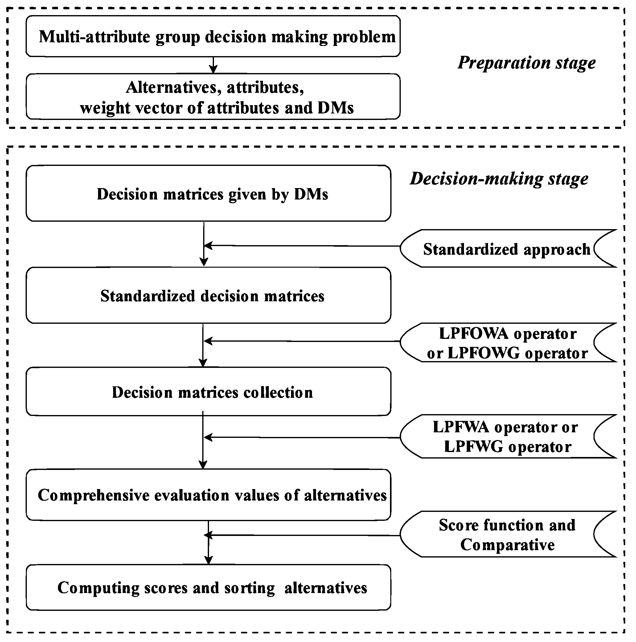
Let ${\rm Y}=\{{{\rm Y}}_1,{{\rm Y}}_2,\dots ,{{\rm Y}}_m\}$ be a group of m alternatives and $\Im =\{{\Im }_1,{\Im }_2,\dots ,{\Im }_n\}$ be a group of attributes whose weight vector $\tau ={({\tau }_1,{\tau }_2,\dots ,{\tau }_n)}^T$, with ${\tau }_j\in [0,1](j=1,2,\dots ,n)$ and ${\sum }_{j=1}^n{\tau }_j=1$. Assume that there is a collection of $\delta$ experts $Z=\{Z_1,Z_2,\dots ,Z_{\delta }\}$ with weight vector $\lambda ={\{{\lambda }_1,{\lambda }_2,\dots ,{\lambda }_{\delta }\}}^T$, with ${\lambda }_k\in [0,1](k=1,2,\dots ,\delta )$ and ${\sum }_{k=1}^{\delta }{\lambda }_k=1$. Expert $Z_k$ provides the evaluation information on alternative $Y_i$ with respect to the attribute ${\Im }_j$ in the form of LPFNs, $q_{ij}^k=(s_{{\alpha }_{ij}}^k,s_{{\beta }_{ij}}^k)$, where $s_{a_{ij}}^k,s_{{\beta }_{ij}}^k\in \overline{S}$. Then the LPF decision matrices $Q^k={\left(q_{ij}^k\right)}_{m\times n}$ are constructed. The decision process is described in the following (the procedure of the propounded MAGDM approach is shown in Figure 1).

Step 1: Normalize the decision matrices. Because there are two kinds of attribute, we need transform them to the same type attribute. That is, normalize the decision matrices $Q^k$ into a normalization matrices $A^k={\left(a_{ij}^k\right)}_{m\times n}$, where

$$a_{ij}=\left\{\begin{array}{cc}(s_{{\alpha }_{ij}}^k,s_{{\beta }_{ij}}^k)\hfill & \mathrm{for}\mathrm{benefit}\mathrm{attribute}{\Im }_{\mathrm{j}}.\hfill \\ (s_{{\beta }_{ij}}^k,s_{{\alpha }_{ij}}^k)\hfill & \mathrm{for}\mathrm{cost}\mathrm{attribute}{\Im }_{\mathrm{j}}.\hfill \end{array}\right.$$

Step 2: Utilize the LPFOWA operator to fuse all the DMs’ information.

$$\begin{array}{c}\hfill q_{ij}=(s_{{\alpha }_{ij}},s_{{\beta }_{ij}})=LPFEOWA(q_{ij}^1,q_{ij}^2,\dots ,q_{ij}^{\delta }),\end{array}$$

or the LPFEOWG operator

$$\begin{array}{c}\hfill q_{ij}=(s_{{\alpha }_{ij}},s_{{\beta }_{ij}})=LPFEOWG(q_{ij}^1,q_{ij}^2,\dots ,q_{ij}^{\delta }).\end{array}$$

Step 3: Utilize the LPFEWA operator to aggregate all $q_{ij}$ for each alternative $Y_i$ as follows.

$$\begin{array}{c}\hfill q_i=LPFWA(q_{i1},q_{i2},\dots ,q_{in})\end{array}$$

or the LPFEWG operators

$$\begin{array}{c}\hfill q_i=LPFEWG(q_{i1},q_{i2},\dots ,q_{in}).\end{array}$$

Step 4: Calculating the score values $\mathcal{T}\left({{\rm Y}}_i\right)$ for each $q_i$.

Step 5: Rank all alternatives ${{\rm Y}}_i(i=1,2,\dots ,m)$.

6. Numerical Example and Comparative Analysis

In this section, we utilize the proposed MAGDM approach to deal with practical problems and perform a comparative analysis to show its effectiveness and merits.

6.1. Numerical Example

Example 1.

This practical example is cited and applied from Reference [57], which is about a company selecting a supplier. Assuming that ${\rm Y}=\{{{\rm Y}}_1,{{\rm Y}}_2,{{\rm Y}}_3,{{\rm Y}}_4\}$ is a set of four optional suppliers as alternatives and the group of attributes $\Im =\{{\Im }_1,{\Im }_2,{\Im }_3,{\Im }_4,{\Im }_5\}$ and the weight of the attribute is $\tau ={(0.25,0.2,0.15,0.18,0.22)}^T$. The alternatives ${\rm Y}=\{{{\rm Y}}_1,{{\rm Y}}_2,{{\rm Y}}_3,{{\rm Y}}_4\}$ are evaluated with respect to the attributes $\Im =\{{\Im }_1,{\Im }_2,{\Im }_3,{\Im }_4,{\Im }_5\}$ by DMs’ using the LPFNs based on the linguistic term set $\mathcal{S}=\{s_0=extremely poor,s_1=very poor,s_2=poor,s_3=slightly poor,s_4=fair,s_5=slightly good,s_6=good,s_7=very good,s_8=extremely good\}$. Assume that the weight vector of DMs’ is $\lambda ={(0.25,0.3,0.2,0.25)}^T$. Then the LPF decision matrices $A_k={\left(a_{ij}^k\right)}_{4\times 5}$ are listed in

Table 1. Decision matrix $Q^1$ by $Z_1$.

	${\mathbf{\Im }}_1$	${\mathbf{\Im }}_2$	${\mathbf{\Im }}_3$	${\mathbf{\Im }}_4$	${\mathbf{\Im }}_5$
${{\rm Y}}_1$	$(s_7,s_1)$	$(s_6,s_2)$	$(s_4,s_3)$	$(s_7,s_1)$	$(s_5,s_2)$
${{\rm Y}}_2$	$(s_6,s_2)$	$(s_5,s_2)$	$(s_6,s_1)$	$(s_6,s_2)$	$(s_7,s_1)$
${{\rm Y}}_3$	$(s_6,s_1)$	$(s_5,s_3)$	$(s_7,s_1)$	$(s_5,s_1)$	$(s_3,s_4)$
${{\rm Y}}_4$	$(s_5,s_2)$	$(s_7,s_1)$	$(s_4,s_3)$	$(s_6,s_1)$	$(s_4,s_4)$

,

Table 2. Decision matrix $Q^2$ by $Z_2$.

	${\mathbf{\Im }}_1$	${\mathbf{\Im }}_2$	${\mathbf{\Im }}_3$	${\mathbf{\Im }}_4$	${\mathbf{\Im }}_5$
${{\rm Y}}_1$	$(s_7,s_1)$	$(s_4,s_4)$	$(s_6,s_2)$	$(s_5,s_1)$	$(s_3,s_5)$
${{\rm Y}}_2$	$(s_7,s_1)$	$(s_5,s_1)$	$(s_6,s_1)$	$(s_5,s_2)$	$(s_4,s_3)$
${{\rm Y}}_3$	$(s_6,s_2)$	$(s_6,s_1)$	$(s_7,s_1)$	$(s_5,s_3)$	$(s_4,s_4)$
${{\rm Y}}_4$	$(s_5,s_2)$	$(s_4,s_3)$	$(s_5,s_2)$	$(s_7,s_1)$	$(s_5,s_3)$

,

Table 3. Decision matrix $Q^3$ by $Z_3$.

	${\mathbf{\Im }}_1$	${\mathbf{\Im }}_2$	${\mathbf{\Im }}_3$	${\mathbf{\Im }}_4$	${\mathbf{\Im }}_5$
${{\rm Y}}_1$	$(s_6,s_1)$	$(s_5,s_2)$	$(s_3,s_4)$	$(s_7,s_1)$	$(s_5,s_2)$
${{\rm Y}}_2$	$(s_7,s_1)$	$(s_6,s_2)$	$(s_7,s_1)$	$(s_6,s_2)$	$(s_5,s_1)$
${{\rm Y}}_3$	$(s_5,s_3)$	$(s_5,s_2)$	$(s_6,s_1)$	$(s_4,s_3)$	$(s_3,s_1)$
${{\rm Y}}_4$	$(s_6,s_2)$	$(s_7,s_1)$	$(s_5,s_1)$	$(s_5,s_2)$	$(s_5,s_4)$

and

Table 4. Decision matrix $Q^4$ by $Z_4$.

	${\mathbf{\Im }}_1$	${\mathbf{\Im }}_2$	${\mathbf{\Im }}_3$	${\mathbf{\Im }}_4$	${\mathbf{\Im }}_5$
${{\rm Y}}_1$	$(s_5,s_3)$	$(s_4,s_4)$	$(s_7,s_1)$	$(s_5,s_1)$	$(s_4,s_2)$
${{\rm Y}}_2$	$(s_6,s_1)$	$(s_7,s_1)$	$(s_6,s_1)$	$(s_5,s_2)$	$(s_6,s_1)$
${{\rm Y}}_3$	$(s_5,s_2)$	$(s_3,s_4)$	$(s_6,s_2)$	$(s_3,s_3)$	$(s_5,s_2)$
${{\rm Y}}_4$	$(s_4,s_3)$	$(s_5,s_1)$	$(s_4,s_2)$	$(s_6,s_2)$	$(s_5,s_2)$

.

Now, we use the proposed approach to cope with this practical problems.

Step 1: The normalization is omitted because all attributes are considered as the benefit attributes.

Step 2: Utilize the LPFOWA operator to aggregate decision matrix $Q^1-Q^4$, the aggregation result is shown in

Table 5. Decision matrix by using LPFOWG operators.

	${\mathbf{\Im }}_1$	${\mathbf{\Im }}_2$	${\mathbf{\Im }}_3$	${\mathbf{\Im }}_4$	${\mathbf{\Im }}_5$
${{\rm Y}}_1$	$(s_{6.4795},s_{1.3229})$	$(s_{4.9191},s_{2.9534})$	$(s_{5.5728},s_{2.2836})$	$(s_{6.3484},s_{1.1908})$	$(s_{4.4073},s_{2.5479})$
${{\rm Y}}_2$	$(s_{6.6295},s_{1.1908})$	$(s_{5.9726},s_{1.4670})$	$(s_{6.3141},s_{1.4670})$	$(s_{5.5985},s_2)$	$(s_{5.8224},s_{1.3229})$
${{\rm Y}}_3$	$(s_{5.2885},s_{1.8690})$	$(s_{4.9355},s_{2.2836})$	$(s_{6.6295},s_{1.1908})$	$(s_{4.4073},s_{2.2962})$	$(s_{3.9091},s_{2.5015})$
${{\rm Y}}_4$	$(s_{5.4217},s_{2.2166})$	$(s_{6.2248},s_{1.3229})$	$(s_{4.5895},s_{1.8690})$	$(s_{6.1317},s_{1.4670})$	$(s_{4.7789},s_{3.1959})$

.

Step 3: Utilize the LPFEWA operator or LPFEWG operator to aggregate all $q_{ij}$ for each alternative ${{\rm Y}}_i$ as follows.

$$\begin{array}{c}\hfill q_1=(s_{5.3862},s_{2.6144}),q_2=(s_{5.6262},s_{2.2769}),q_3=(s_{4.8177},s_{2.7532}),q_4=(s_{5.1312},s_{2.5480}).\end{array}$$

Step 4: According to the score function to calculate the score value of each alternative ${{\rm Y}}_i(i=1,2,3,4)$;

$$\begin{array}{c}\hfill \mathcal{T}\left(q_1\right)=6.5641,\mathcal{T}\left(q_2\right)=6.7257,\mathcal{T}\left(q_3\right)=6.3099,\mathcal{T}\left(q_4\right)=6.4744.\end{array}$$

Step 5: the order relation of alternative ${{\rm Y}}_i(i=1,2,\dots ,4)$ is obtained as follows: ${{\rm Y}}_2\succ {{\rm Y}}_1\succ {{\rm Y}}_4\succ {{\rm Y}}_3$. Hence, the best alternative is ${{\rm Y}}_2$.

Example 2.

This example is cited from Reference [60]. The following example is that a multinational company is planning the strategic objectives of its financial strategy group for the next year and expanding it to other countries. To this end, the planning department after consultation is to provide four strategic options for selection, which is depicted as follows:

1. 

${{\rm Y}}_1$: Expand to Asia;

2. 

${{\rm Y}}_2$: Expand to African;

3. 

${{\rm Y}}_3$: Expand to Northern American;

4. 

${{\rm Y}}_4$: Expand to all three continent.

In order to evaluate the given alternatives, the company considers the following factors as the attributes of alternatives which are shown as follows:

1. 

${\Im }_1$: Short term interests;

2. 

${\Im }_2$: Medium-term interest;

3. 

${\Im }_3$: Long-term interests;

4. 

${\Im }_4$: Strategic risk.

In order to acquire the best alternative, the company invited three strategic decision experts $Z_1,Z_2,Z_3$ to provide their evaluation information for each alternative with respect to the given attribute by the linguistic term set $\overline{\mathcal{S}}=\{s_0=\mathrm{extremely} \mathrm{poor},s_1=\mathrm{very} \mathrm{poor},s_2=\mathrm{poor},s_3=\mathrm{slightly} \mathrm{poor},s_4=\mathrm{fair},s_5=\mathrm{slightly} \mathrm{good},s_6=\mathrm{good},s_7=\mathrm{very} \mathrm{good},s_8=\mathrm{extremely} \mathrm{good}\}$. Then the LPF decision matrices $R^1$, $R^2$ and $R^3$ are listed in

Table 6. Decision matrix $R^1$ by expert $Z_1$.

	${\mathbf{\Im }}_1$	${\mathbf{\Im }}_2$	${\mathbf{\Im }}_3$	${\mathbf{\Im }}_4$
${{\rm Y}}_1$	$(s_6,s_1)$	$(s_3,s_1)$	$(s_3,s_3)$	$(s_1,s_6)$
${{\rm Y}}_2$	$(s_3,s_4)$	$(s_3,s_4)$	$(s_2,s_5)$	$(s_2,s_4)$
${{\rm Y}}_3$	$(s_1,s_3)$	$(s_2,s_3)$	$(s_3,s_2)$	$(s_6,s_1)$
${{\rm Y}}_4$	$(s_6,s_2)$	$(s_4,s_3)$	$(s_5,s_1)$	$(s_7,s_1)$

,

Table 7. Decision matrix $R^2$ by expert $Z_2$.

	${\mathbf{\Im }}_1$	${\mathbf{\Im }}_2$	${\mathbf{\Im }}_3$	${\mathbf{\Im }}_4$
${{\rm Y}}_1$	$(s_3,s_2)$	$(s_3,s_1)$	$(s_3,s_4)$	$(s_2,s_3)$
${{\rm Y}}_2$	$(s_5,s_2)$	$(s_2,s_1)$	$(s_3,s_4)$	$(s_2,s_5)$
${{\rm Y}}_3$	$(s_2,s_3)$	$(s_2,s_3)$	$(s_1,s_2)$	$(s_3,s_3)$
${{\rm Y}}_4$	$(s_5,s_2)$	$(s_4,s_3)$	$(s_5,s_2)$	$(s_4,s_1)$

and

Table 8. Decision matrix $R^3$ by expert $Z_3$.

	${\mathbf{\Im }}_1$	${\mathbf{\Im }}_2$	${\mathbf{\Im }}_3$	${\mathbf{\Im }}_4$
${{\rm Y}}_1$	$(s_3,s_3)$	$(s_3,s_5)$	$(s_6,s_1)$	$(s_2,s_6)$
${{\rm Y}}_2$	$(s_3,s_2)$	$(s_2,s_4)$	$(s_2,s_1)$	$(s_3,s_4)$
${{\rm Y}}_3$	$(s_6,s_1)$	$(s_2,s_5)$	$(s_3,s_4)$	$(s_1,s_3)$
${{\rm Y}}_4$	$(s_5,s_1)$	$(s_4,s_4)$	$(s_6,s_2)$	$(s_5,s_2)$

. The associated weight vector of attributes is $\tau =(0.3,0.1,0.2,0.4)$. Next, the best alternative is selected by utilizing the proposed approach and the detailed steps are described below:

Step 1: The normalization is omitted because all attributes are considered benefit attributes.

Step 2: Utilize the LPFOWA operator to aggregate decision matrix $R^1-R^3$, the aggregation result is shown in

Table 9. Decision matrix by using LPFOWG operators.

	${\mathbf{\Im }}_1$	${\mathbf{\Im }}_2$	${\mathbf{\Im }}_3$	${\mathbf{\Im }}_4$
${{\rm Y}}_1$	$(s_{3.6051},s_{2.1203})$	$(s_{3.2221},s_{2.6726})$	$(s_{3.6015},s_{2.9691})$	$(s_{1.6928},s_{5.5123})$
${{\rm Y}}_2$	$(s_{3.4175},s_{2.6413})$	$(s_{2.2102},s_{3.6176})$	$(s_{2.3137},s_{2.6413})$	$(s_{2.7965},s_{2.6594})$
${{\rm Y}}_3$	$(s_{2.2713},s_{2.6594})$	$(s_{2.2102},s_{3.6176})$	$(s_{2.3137},s_{2.6413})$	$(s_{2.7965},s_{2.6594})$
${{\rm Y}}_4$	$(s_{5.2362},s_{1.8089})$	$(s_{3.7361},s_{3.2754})$	$(s_{5.2362},s_{1.8089})$	$(s_{5.2015},s_{1.3153})$

.

Step 3: Utilize the LPFEWA operator or LPFEWG operator to aggregate all $q_{ij}$ for each alternative ${{\rm Y}}_i$ as follows.

$$\begin{array}{c}\hfill q_1=(s_{2.6532},s_{1.9591}),q_2=(s_{2.7984},s_{2.5207}),q_3=(s_{2.4721},s_{2.2021}),q_4=(s_{5.0590},s_{1.6489}).\end{array}$$

Step 4: According to the score function to compute the score value of each alternative $q_i(i=1,2,3,4)$

$$\begin{array}{c}\hfill \mathcal{T}\left(q_1\right)=5.7966,\mathcal{T}\left(q_2\right)=5.7218,\mathcal{T}\left(q_3\right)=5.7142,\mathcal{T}\left(q_4\right)=6.5907.\end{array}$$

Step 5: By the comparison laws defined in Definition 2, the order relation of alternative ${{\rm Y}}_i(i=1,2,3,4)$ is obtained as follows: ${{\rm Y}}_4\succ {{\rm Y}}_1\succ {{\rm Y}}_2\succ {{\rm Y}}_3$. Hence, the best alternative is ${{\rm Y}}_4$.

6.2. Comparative Analysis

In order to verify the validity and practicability of the developed method and to analyze its merits in this article, we compare the proposed method with the existing approaches, including the method based on linguistic intuitionistic fuzzy weighted average operator proposed by Chen et al. [57], the method based on linguistic intuitionistic fuzzy Einstein weighted average (LIFEWA) operator proposed by Garg [58] and the method based on LPF weighted average operator proposed by Garg [60]. We utilize the proposed approach to resolve the application examples in the existing methods, the final sorting results are displayed in

Table 10. A comparison of preference order for different approaches.

	Ranking Orders	Ranking Orders
	in the Original Literature	Based on Proposed Approach
Example in [57]	${{\rm Y}}_2\succ {{\rm Y}}_1\succ {{\rm Y}}_4\succ {{\rm Y}}_3$	${{\rm Y}}_2\succ {{\rm Y}}_1\succ {{\rm Y}}_4\succ {{\rm Y}}_3$
Example in [58]	${{\rm Y}}_2\succ {{\rm Y}}_1\succ {{\rm Y}}_4\succ {{\rm Y}}_3$	${{\rm Y}}_2\succ {{\rm Y}}_1\succ {{\rm Y}}_4\succ {{\rm Y}}_3$
Example in [60]	${{\rm Y}}_4\succ {{\rm Y}}_3\succ {{\rm Y}}_1\succ {{\rm Y}}_2$	${{\rm Y}}_4\succ {{\rm Y}}_3\succ {{\rm Y}}_1\succ {{\rm Y}}_2$

. From Table 10, it is apparent that the ranking results obtained by the proposed method are same as those of the existing methods. That proves the validity of the propounded approach in this article. In what follows, the advantages of the proposed method are demonstrated through a detailed comparison with above-mentioned methods.

(1) Compared with the method based on LIFWA operator propounded by Chen et al. [57], although the LIFWA operator can be utilized to aggregate fuzzy and uncertain information, it lakes flexibility and robustness during the information fusion process because its operational laws are generated by Algebraic T-norm and S-norm. Besides, the LIFN can not address several special situations in real-life issues. For instance, if an expert provides his or her preference information in the form of LIFN denoted as $(s_5,s_6)$ with $s_6,s_5\in \mathcal{S}$, we can find that the LIFWA operator fails to resolve situation because of $5+6\nleqq 8$. However, the approach based on the LPFEWA operator can overcome the above defects. The operational rules generated by Einstein T-norm and S-norm can improve the robustness and smoothness, the LPFS can address the special situation because of $5^2+6^2\le 8^2$. Accordingly, the presented approach in this paper is more general and flexible at resolving actual issues than LIFN.

(2) Compared with the method based on the LIFEWA operator propounded by Garg [58], the evaluation information of the approach is in the form of LPFN. We can find that the sorting result of alternatives in the Example is ${{\rm Y}}_2\succ {{\rm Y}}_1\succ {{\rm Y}}_4\succ {{\rm Y}}_3$, which is the same as with the method in Reference [58]. However, if the decision maker $Z_1$ in Example 1 changes his preference information for alternative ${{\rm Y}}_1$ with respect to ${\Im }_1$ and ${\Im }_2$ to $(s_4,s_5)$ and $(s_3,s_7)$, respectively, we cannot acquire the score values and ranking relation of the alternative by utilizing the LIFEWA operator. For this limitation, the LPFEWA operator can efficiently overcome it and attain the final sorting of alternatives. Hence, the LPFS can provide more freedom for the evaluator to express their assessment information in practical problems.

(3) Compared with the method based on the LPFWA operator propounded by Garg [60], the LPFWA operator is obtained on the basis of Algebraic T-norm and S-norm. The proposed approach based upon the LPFEWA operator is generated through Einstein T-norm and S-norm, which has more robustness and smoothness than Algebraic operations.

To sum up, the developed approach fully demonstrates flexibility and effectiveness by combining LPFS and Einstein operation. It is more general than LIFS and PFS in solving practical problems. The significant characteristics of the proposed and other existing approaches are summarized in

Table 11. Feature comparison for different methods.

Approaches	Whether Quantitative Description of Information	Whether Qualitative Description of Information	Describe a Wider Range of Information	Have Generalized Features
The method propounded by Xu in [17]	NO	NO	NO	NO
The method propounded by Xia et al. in [18]	NO	NO	NO	YES
The method propounded by Chen et al. in [57]	YES	YES	NO	YES
The method propounded by Garg in [60]	YES	YES	YES	NO
The propounded method in this paper	YES	YES	YES	YES

.

7. Conclusions

LPFS is the extension of PFS, where membership degree and nonmembership degree are indicated by the linguistic terms to process vague information from a qualitative point of view. In this article, we propose a multi-attribute group decision making approach for dealing with decision making problems. To begin with, we define the novel operational laws of LPFNs by utilizing the Einstein operation. Thereafter, we present several novel LPF Einstein averaging and geometric aggregation operators to fuse the diverse assessment information of alternatives. Some desirable properties of these aggregation operators are discussed in detail. Moreover, we utilize these aggregation operators to construct a novel decision making method to tackle practical issues with LPF information. Two illustration examples are utilized to demonstrate the validity and practicality of the proposed method. A comparative analysis with existing methods is carried out to display the superiorities of the presented approach. In future research, we will further investigate the Einstein operations in other fuzzy environments such as linguistic single-valued neutrosophic sets [64], picture 2-tuple linguistic sets [65] and so on. Furthermore, we can apply the propounded aggregation operators to solve practical issues, such as information fusion, knowledge management and risk evaluation. At the same time, we will continue to consider the theory of linguistic Pythagorean fuzzy sets and its methodologies and applications in decision support systems, big data analysis and so on.

References

- Pei, Z.; Liu, J.; Hao, F.; Zhou, B. FLM-TOPSIS: The fuzzy linguistic multiset TOPSIS method and its application in linguistic decision making. Inf. Fusion 2019, 45, 266–281. [Google Scholar] [CrossRef]
- Garg, H.; Kaur, G. Quantifying gesture information in brain hemorrhage patients using probabilistic dual hesitant fuzzy sets with unknown probability information. Comput. Ind. Eng. 2020, 140, 106211. [Google Scholar] [CrossRef]
- Garg, H.; Chen, S.M. Multiattribute group decision making based on neutrality aggregation operators of q-rung orthopair fuzzy sets. Inf. Sci. 2019. [Google Scholar] [CrossRef]
- Peng, X.; Dai, J.; Garg, H. Exponential operation and aggregation operator for q-rung orthopair fuzzy set and their decision-making method with a new score function. Int. J. Intell. Syst. 2018, 33, 2255–2282. [Google Scholar] [CrossRef]
- Liu, Y.; Liu, J.; Hong, Z. A multiple attribute decision making approach based on new similarity measures of interval-valued hesitant fuzzy sets. Int. J. Comput. Intell. Syst. 2018, 11, 15–32. [Google Scholar] [CrossRef] [Green Version]
- Liu, Y.; Qin, Y.; Han, Y. Multiple criteria decision making with probabilities in interval-valued Pythagorean fuzzy setting. Int. J. Fuzzy Syst. 2018, 20, 558–571. [Google Scholar] [CrossRef]
- Zadeh, L.A. Fuzzy sets. Inf. Control 1965, 8, 338–353. [Google Scholar] [CrossRef] [Green Version]
- Li, Y.; Sui, S.; Tong, S. Adaptive fuzzy control design for stochastic nonlinear switched systems with arbitrary switchings and unmodeled dynamics. IEEE Trans. Cybern. 2016, 47, 403–414. [Google Scholar] [CrossRef]
- Wang, Y.; Shen, H.; Karimi, H.R.; Duan, D. Dissipativity-based fuzzy integral sliding mode control of continuous-time TS fuzzy systems. IEEE Trans. Fuzzy Syst. 2017, 26, 1164–1176. [Google Scholar]
- Ferdaus, M.M.; Pratama, M.; Anavatti, S.; Garratt, M.A.; Pan, Y. Generic evolving self-organizing neuro-fuzzy control of bio-inspired unmanned aerial vehicles. IEEE Trans. Fuzzy Syst. 2019. [Google Scholar] [CrossRef] [Green Version]
- Joshi, D.; Kumar, S. Interval-valued intuitionistic hesitant fuzzy Choquet integral based TOPSIS method for multi-criteria group decision making. Eur. J. Oper. Res. 2016, 248, 183–191. [Google Scholar] [CrossRef]
- Garg, H. Distance and similarity measures for intuitionistic multiplicative preference relation and its applications. Int. J. Uncertain. Quantif. 2017, 7, 117–133. [Google Scholar] [CrossRef]
- Sun, B.; Ma, W.; Li, B.; Li, X. Three-way decisions approach to multiple attribute group decision making with linguistic information-based decision-theoretic rough fuzzy set. Int. J. Approx. Reason. 2018, 93, 424–442. [Google Scholar] [CrossRef]
- Garg, H. Some methods for strategic decision-making problems with immediate probabilities in Pythagorean fuzzy environment. Int. J. Intell. Syst. 2018, 33, 687–712. [Google Scholar] [CrossRef]
- Dincer, H.; Yüksel, S.; Martinez, L. Balanced scorecard-based Analysis about European Energy Investment Policies: A hybrid hesitant fuzzy decision-making approach with Quality Function Deployment. Expert Syst. Appl. 2019, 115, 152–171. [Google Scholar] [CrossRef]
- Atanassov, K.T. Intuitionistic fuzzy sets. Fuzzy Sets Syst. 1986, 20, 87–96. [Google Scholar] [CrossRef]
- Xu, Z. Intuitionistic fuzzy aggregation operators. IEEE Trans. Fuzzy Syst. 2007, 15, 1179–1187. [Google Scholar]
- Xia, M.; Xu, Z.; Zhu, B. Some issues on intuitionistic fuzzy aggregation operators based on Archimedean t-conorm and t-norm. Knowl.-Based Syst. 2012, 31, 78–88. [Google Scholar] [CrossRef]
- Abdullah, L.; Zulkifli, N.; Liao, H.; Herrera-Viedma, E.; Al-Barakati, A. An interval-valued intuitionistic fuzzy DEMATEL method combined with Choquet integral for sustainable solid waste management. Eng. Appl. Artif. Intell. 2019, 82, 207–215. [Google Scholar] [CrossRef]
- Zhang, D.; Li, Y.; Wu, C. An extended TODIM method to rank products with online reviews under intuitionistic fuzzy environment. J. Oper. Res. Soc. 2019, 71, 322–334. [Google Scholar] [CrossRef]
- Shen, F.; Ma, X.; Li, Z.; Xu, Z.; Cai, D. An extended intuitionistic fuzzy TOPSIS method based on a new distance measure with an application to credit risk evaluation. Inf. Sci. 2018, 428, 105–119. [Google Scholar] [CrossRef]
- Liu, P.; Liu, J.; Chen, S.M. Some intuitionistic fuzzy Dombi Bonferroni mean operators and their application to multi-attribute group decision making. J. Oper. Res. Soc. 2018, 69, 1–24. [Google Scholar] [CrossRef]
- Liu, Y.; Liu, J.; Qin, Y. Dynamic intuitionistic fuzzy multiattribute decision making based on evidential reasoning and MDIFWG operator. J. Intell. Fuzzy Syst. 2019, 36, 2161–2172. [Google Scholar] [CrossRef]
- Yager, R.R. Pythagorean membership grades in multicriteria decision making. IEEE Trans. Fuzzy Syst. 2013, 22, 958–965. [Google Scholar] [CrossRef]
- Yager, R.R.; Abbasov, A.M. Pythagorean membership grades, complex numbers, and decision making. Int. J. Intell. Syst. 2013, 28, 436–452. [Google Scholar] [CrossRef]
- Garg, H. Neutrality operations-based Pythagorean fuzzy aggregation operators and its applications to multiple attribute group decision-making process. J. Ambient Intell. Hum. Comput. 2019, 1–21. [Google Scholar] [CrossRef]
- Garg, H. New logarithmic operational laws and their aggregation operators for Pythagorean fuzzy set and their applications. Int. J. Intell. Syst. 2019, 34, 82–106. [Google Scholar] [CrossRef] [Green Version]
- Peng, X.; Dai, J. Approaches to Pythagorean fuzzy stochastic multi-criteria decision making based on prospect theory and regret theory with new distance measure and score function. Int. J. Intell. Syst. 2017, 32, 1187–1214. [Google Scholar] [CrossRef]
- Garg, H. A new improved score function of an interval-valued Pythagorean fuzzy set based TOPSIS method. Int. J. Uncertain. Quantif. 2017, 7. [Google Scholar] [CrossRef]
- Peng, X.; Yuan, H.; Yang, Y. Pythagorean fuzzy information measures and their applications. Int. J. Intell. Syst. 2017, 32, 991–1029. [Google Scholar] [CrossRef]
- Xue, W.; Xu, Z.; Zhang, X.; Tian, X. Pythagorean fuzzy LINMAP method based on the entropy theory for railway project investment decision making. Int. J. Intell. Syst. 2018, 33, 93–125. [Google Scholar] [CrossRef]
- Rani, P.; Mishra, A.R.; Pardasani, K.R.; Mardani, A.; Liao, H.; Streimikiene, D. A novel VIKOR approach based on entropy and divergence measures of Pythagorean fuzzy sets to evaluate renewable energy technologies in India. J. Clean. Prod. 2019, 238, 117936. [Google Scholar] [CrossRef]
- Qin, Y.; Liu, Y.; Hong, Z. Multicriteria decision making method based on generalized Pythagorean fuzzy ordered weighted distance measures. J. Intell. Fuzzy Syst. 2017, 33, 3665–3675. [Google Scholar] [CrossRef]
- Zeng, W.; Li, D.; Yin, Q. Distance and similarity measures of Pythagorean fuzzy sets and their applications to multiple criteria group decision making. Int. J. Intell. Syst. 2018, 33, 2236–2254. [Google Scholar] [CrossRef]
- Li, D.; Zeng, W. Distance measure of Pythagorean fuzzy sets. Int. J. Intell. Syst. 2018, 33, 348–361. [Google Scholar] [CrossRef]
- Peng, X.; Garg, H. Multiparametric similarity measures on Pythagorean fuzzy sets with applications to pattern recognition. Appl. Intell. 2019, 49, 4058–4096. [Google Scholar] [CrossRef]
- Li, Z.; Lu, M. Some novel similarity and distance measures of pythagorean fuzzy sets and their applications. J. Intell. Fuzzy Syst. 2019, 37, 1781–1799. [Google Scholar] [CrossRef]
- Peng, X.; Yang, Y. Pythagorean fuzzy Choquet integral based MABAC method for multiple attribute group decision making. Int. J. Intell. Syst. 2016, 31, 989–1020. [Google Scholar] [CrossRef]
- Liang, D.; Xu, Z.; Liu, D.; Wu, Y. Method for three-way decisions using ideal TOPSIS solutions at Pythagorean fuzzy information. Inf. Sci. 2018, 435, 282–295. [Google Scholar] [CrossRef]
- Khan, M.S.A.; Abdullah, S.; Ali, A.; Amin, F. An extension of VIKOR method for multi-attribute decision-making under Pythagorean hesitant fuzzy setting. Granul. Comput. 2019, 4, 421–434. [Google Scholar] [CrossRef]
- Garg, H. Generalized Pythagorean fuzzy geometric aggregation operators using Einstein t-norm and t-conorm for multicriteria decision-making process. Int. J. Intell. Syst. 2017, 32, 597–630. [Google Scholar] [CrossRef]
- Garg, H. Novel neutrality operation–based Pythagorean fuzzy geometric aggregation operators for multiple attribute group decision analysis. Int. J. Intell. Syst. 2019, 34, 2459–2489. [Google Scholar] [CrossRef]
- Li, N.; Garg, H.; Wang, L. Some Novel Interactive Hybrid Weighted Aggregation Operators with Pythagorean Fuzzy Numbers and Their Applications to Decision Making. Mathematics 2019, 7, 1150. [Google Scholar] [CrossRef] [Green Version]
- Zhu, J.; Li, Y. Pythagorean fuzzy Muirhead mean operators and their application in multiple-criteria group decision-Making. Information 2018, 9, 142. [Google Scholar] [CrossRef] [Green Version]
- Khan, A.A.; Abdullah, S.; Shakeel, M.; Khan, F.; Luo, J. A New Ranking Methodology for Pythagorean Trapezoidal Uncertain Linguistic Fuzzy Sets Based on Einstein Operations. Symmetry 2019, 11, 440. [Google Scholar] [CrossRef] [Green Version]
- Gao, H.; Lu, M.; Wei, G.; Wei, Y. Some novel Pythagorean fuzzy interaction aggregation operators in multiple attribute decision making. Fundam. Inform. 2018, 159, 385–428. [Google Scholar] [CrossRef]
- Joshi, B.P. Pythagorean fuzzy average aggregation operators based on generalized and group-generalized parameter with application in MCDM problems. Int. J. Intell. Syst. 2019, 34, 895–919. [Google Scholar] [CrossRef]
- Biswas, A.; Sarkar, B. Interval-valued Pythagorean fuzzy TODIM approach through point operator-based similarity measures for multicriteria group decision making. Kybernetes 2019, 48, 496–519. [Google Scholar] [CrossRef]
- Khan, M.S.A.; Abdullah, S. Interval-valued Pythagorean fuzzy GRA method for multiple-attribute decision making with incomplete weight information. Int. J. Intell. Syst. 2018, 33, 1689–1716. [Google Scholar] [CrossRef]
- Ali Khan, M.S.; Abdullah, S.; Ali, A. Multiattribute group decision-making based on Pythagorean fuzzy Einstein prioritized aggregation operators. Int. J. Intell. Syst. 2019, 34, 1001–1033. [Google Scholar] [CrossRef]
- Shakeel, M.; Abdullah, S.; Shahzad, M.; Amin, F.; Mahmood, T.; Amin, N. Pythagorean trapezoidal fuzzy geometric aggregation operators based on Einstein operations and their application in group decision making. Intell. Fuzzy Syst. 2019, 36, 309–324. [Google Scholar] [CrossRef]
- Zadeh, L.A. The concept of a linguistic variable and its application to approximate reasoning—I. Inf. Sci. 1975, 8, 199–249. [Google Scholar] [CrossRef]
- Zadeh, L.A. The concept of a linguistic variable and its application to approximate reasoning—II. Inf. Sci. 1975, 8, 301–357. [Google Scholar] [CrossRef]
- Zadeh, L.A. The concept of a linguistic variable and its application to approximate reasoning—III. Inf. Sci. 1975, 9, 43–80. [Google Scholar] [CrossRef]
- Xu, Z. Deviation measures of linguistic preference relations in group decision making. Omega 2005, 33, 249–254. [Google Scholar] [CrossRef]
- Zhang, H. Linguistic intuitionistic fuzzy sets and application in MAGDM. J. Appl. Math. 2014, 2014, 432092. [Google Scholar] [CrossRef] [Green Version]
- Chen, Z.; Liu, P.; Pei, Z. An approach to multiple attribute group decision making based on linguistic intuitionistic fuzzy numbers. Int. J. Comput. Intell. Syst. 2015, 8, 747–760. [Google Scholar] [CrossRef] [Green Version]
- Garg, H.; Kumar, K. Group Decision Making Approach Based on Possibility Degree Measures and the Linguistic Intuitionistic Fuzzy Aggregation Operators Using Einstein Norm Operations. J. Mult.-Valued Logic Soft Comput. 2018, 31, 175–209. [Google Scholar]
- Garg, H.; Kumar, K. Linguistic interval-valued Atanassov intuitionistic fuzzy sets and their applications to group decision-making problems. IEEE Trans. Fuzzy Syst. 2019, 27, 2302–2311. [Google Scholar] [CrossRef]
- Garg, H. Linguistic Pythagorean fuzzy sets and its applications in multiattribute decision-making process. Int. J. Intell. Syst. 2018, 33, 1234–1263. [Google Scholar] [CrossRef]
- Lin, M.; Wei, J.; Xu, Z.; Chen, R. Multiattribute Group Decision-Making Based on Linguistic Pythagorean Fuzzy Interaction Partitioned Bonferroni Mean Aggregation Operators. Complexity 2018, 2018, 9531064. [Google Scholar] [CrossRef] [Green Version]
- Lin, M.; Huang, C.; Xu, Z. TOPSIS Method Based on Correlation Coefficient and Entropy Measure for Linguistic Pythagorean Fuzzy Sets and Its Application to Multiple Attribute Decision Making. Complexity 2019, 2019, 6967390. [Google Scholar] [CrossRef]
- Klement, E.P.; Mesiar, R.; Pap, E. Problems on triangular norms and related operators. Fuzzy Sets Syst. 2004, 145, 471–479. [Google Scholar] [CrossRef]
- Garg, H. Linguistic single-valued neutrosophic power aggregation operators and their applications to group decision-making problems. IEEE/CAA J. Autom. Sin. 2019. [Google Scholar] [CrossRef]
- Wei, G.; Alsaadi, F.E.; Hayat, T.; Alsaedi, A. Picture 2-tuple linguistic aggregation operators in multiple attribute decision making. Soft Comput. 2018, 22, 989–1002. [Google Scholar] [CrossRef]
Figure 1.
The decision process of the propounded MAGDM approach.