An Efficient Adaptive Traffic Light Control System for Urban Road Traffic Congestion Reduction in Smart Cities


Department of Computing and Mathematics, Manchester Metropolitan University, Manchester M15 6BH, UK
*
Author to whom correspondence should be addressed.
†
These authors contributed equally to this work.
Information 2020, 11(2), 119; https://0-doi-org.brum.beds.ac.uk/10.3390/info11020119
Submission received: 13 January 2020
/
Revised: 12 February 2020
/
Accepted: 17 February 2020
/
Published: 21 February 2020
(This article belongs to the Special Issue Emerging Topics in Wireless Communications for Future Smart Cities)
Abstract
:Traffic lights have been used for decades to control and manage traffic flows crossing road intersections to increase traffic efficiency and road safety. However, relying on fixed time cycles may not be ideal in dealing with the increasing congestion level in cities. Therefore, we propose a new Adaptive Traffic Light Control System (ATLCS) to assist traffic management authorities in efficiently dealing with traffic congestion in cities. The main idea of our ATLCS consists in synchronizing a number of traffic lights controlling consecutive junctions by creating a delay between the times at which each of them switches to green in a given direction. Such a delay is dynamically updated based on the number of vehicles waiting at each junction, thereby allowing vehicles leaving the city centre to travel a long distance without stopping (i.e., minimizing the number of occurrences of the ‘stop and go’ phenomenon), which in turn reduces their travel time as well. The performance evaluation of our ATLCS has shown that the average travel time of vehicles traveling in the synchronized direction has been significantly reduced (by up to 39%) compared to non-synchronized fixed time Traffic Light Control Systems. Moreover, the overall achieved improvement across the simulated road network was 17%.
1. Introduction
The concept of the Smart City has emerged in recent years as a futuristic vision of cities building sustainable ecosystems, while promoting citizen welfare and economic growth. A Smart City fosters the use of advanced ubiquitous information communication technologies (ICTs) to smartly and efficiently monitor and manage its critical assets such as energy, water, and transportation infrastructure. Such an ambition can become a reality only with joint efforts from governmental, industrial, academic and social actors. Building smart cities, however, strongly depends on various enabling advanced technologies (e.g., sensors, Internet of Things (IoT), 5G networks, the cloud, Artificial Intelligence, connected vehicles, etc.) to support sustainable developments such as smart buildings and energy, and smart and green transportation. Smart and Green Transportation Systems (SGTS) are considered a main pillar of smart cities since the efficiency of several services are reliant on their level of robustness and security [1]. Transport experts foresee that SGTS will be mainly comprised of automated or autonomous vehicles, as well as cutting-edge transportation infrastructure and innovative applications. Such an infrastructure includes advanced traffic light controllers, cutting-edge traffic monitoring equipment and sensing devices, etc. The main mission of a SGTS is to efficiently control and mitigate road traffic congestion problem that most of cities suffer from.
The excessive traffic congestion we see everyday, especially in urban areas, is primarily due to the increase in the number of vehicles in circulation which in turn causes accidents and worsens the congestion level of the already deteriorated road network infrastructure. Traffic congestion has major impacts on the environment, the economy and the population’s health [2]. Numerous studies have been conducted in the last decades to improve the traffic flow fluidity, especially during peak hours. Although some of the developed solutions have already been implemented in many big cities across the world and led to a non negligible improvement of traffic congestion control and mitigation efficiency, there is still a lot to be done as traffic congestion remains a serious problem with a detrimental impact. The INRIX Global Traffic Scorecard [3] published the results of their research on the impact of congestion during the year 2016 in more than a thousand cities around the world. From the 38 countries involved, the United Kingdom (UK) is the 4th most congested with an estimation of 32 h wasted annually per driver during peak hours. The congestion impact on the economy is staggering as direct and indirect cost altogether in the UK were estimated to be around £30.8 billion in 2016 which translates to around £968 per driver. Indirect costs are estimated to be 12% of the total cost. When it comes to London alone, the most congested city in the UK, the 2nd in Europe (behind Moscow) and the 7th in the world, these figures get even worse as in 2016 each driver wasted on average 73 h during peak hours, more than double the UK average. The annual congestion cost per driver in London was estimated to be £1911, which translates to £6.2 billion for the whole city. Traffic congestion also has a major impact on the environment because vehicles that are idling or moving at low speed create unnecessary air pollution through the emission of carbon dioxide which has the negative impact on global warming.
The last two decades have witnessed an unprecedented revolution in developing advanced ICT driven solutions to mitigate increasing road traffic congestion and alleviate its resulting impact on travellers’ journey experience, road safety, air quality and economy. To contribute to these efforts and support the existing SGTSs we design in this paper a novel synchronization algorithm to be used by Traffic Light Control Systems (TLCSs) deployed at intersections of arterial roads connected to city centres. The main idea consists in adapting the traffic light cycles duration based on the traffic flow crossing arterial roads while exiting the city centre during afternoon peak hours, which in turn should reduce congestion in city centres. Please note that this work is an extension of our recently accepted conference paper at [4], where we have added more technical details and illustrations about the proposed system, a detailed discussion of the related works and extensive simulation results.
The main contributions of this paper can be summarised as follows:
- Developing an efficient yet cheap and easy to deploy Adaptive Traffic Light Control System (ATLCS) to quickly reduce traffic congestion in city centres during afternoon peak hours.
- Minimising the number of “stop and go” events occurring during a vehicle travel across arterial roads connected to city centres. This is a direct consequence of the developed synchronisation algorithm since the synchronisation is achieved by computing the required delay for switching to the green phase between consecutive traffic lights. Such a delay is computed based on the length of the queue of vehicles waiting at each intersection. Thereby, the stop and go time is minimised.
- Demonstrating the efficiency of our ATLCS through conducting extensive simulation using the most widely used microscopic traffic simulator, SUMO. This includes 50 simulation runs for every scenario to collect statistically representative results.
The remainder of this paper is organized as follows. Section 2 briefly reviews some existing works. Section 3 presents the fundamentals of our solution along with its detailed operation. In Section 4, we evaluate the performance of our solution and analyze the obtained simulation results. Finally, we conclude the paper in Section 5.
2. Related Work
In this section we will briefly discuss the main idea of some recent ICT driven approaches that dealt with traffic congestion problem.
The work introduced in Reference [5] aims at minimizing traffic congestion and air pollution by analyzing, in real-time, the speed of vehicles crossing road intersections. For the sake of simplicity, the authors assume that all vehicles run straight and never turn left or right. In this work, every vehicle that crosses a junction, from both directions (North-South and East-West), sends to the traffic light controlling it its location, speed, direction and other details. The traffic light in return analyzes the received messages and decides according to a defined algorithm whether to extend or shorten the length of the current phase. Although the authors state that this solution outperforms traffic lights control systems with fixed phase length in terms of the throughput of vehicles crossing the different junctions there is no simulation nor analytical evaluation presented to support this assertion.
The delay of emergency vehicles, such as ambulances and firefighter trucks, is, no doubt, among the most critical consequences of traffic congestion as it may lead to substantial losses of assets and human lives. To overcome this issue, the authors of Reference [6] proposed an advanced adaptive traffic control system built upon a fuzzy logic controller that combines the observed road occupancy level and average speed to assess the current congestion level. This latter, along with the announced emergency level, are used to determine the most effective emergency response plan that helps the emergency vehicle to get to the emergency location with minimum delay. Such a plan could vary from adapting the traffic light cycles duration to temporarily changing the driving policies and re-routing a number of selected vehicles to clear the route for the emergency vehicle. The evaluation results have proven the effectiveness of this system as the reduction of emergency vehicles’ response time was significant while the disruption caused to the non-emergency vehicles was negligible. The efficiency of this system could be further tested in different weather conditions, times of the day or by investigating the impact of the presence of stalled or crashed vehicles on the emergency vehicle road.
Another work published in Reference [7] aims at reducing the average waiting time at a junction while avoiding starvation. This latter represents a situation where a traffic signal of one direction does not switch to green for a relatively long period of time. The proposed solution uses two magnetometer sensors per incoming lane, one is positioned close to the traffic light and the other further behind at a distance that would, in theory, accommodate the number of vehicles that could cross the junction if the green light duration was set to its maximum value. The deployed sensors are grouped into four different hierarchical levels, where sensors of each level are assigned specific tasks to distribute the computation load since sensors could be battery powered. The main particularity of this solution is, as opposed to common approaches that set the whole cycle in advance, the lack of cycles notion as the next phase is decided by analyzing the data received by sensors during the current phase. This solution is very flexible as it could be adapted to any road junction by configuring all possible movements per direction. The selection of the next phase duration is defined based on two factors, the queue-length and the risk of starvation. The method used to determine the green light duration mainly depends on the number of vehicles in the most occupied lane. A better approach might be to take into account the number of vehicles present on all incoming lanes instead as this may enhance the overall road network efficiency. The above work has been extended in Reference [8] by developing a decentralized multi-junction adaptive traffic lights control algorithm named TAPIOCA (distribuTed and AdaPtive Intersections Control Algorithm) that aims to reduce the average waiting time at junctions, prioritize phases leading to less congested roads and favour phases that could potentially lead to adjacent traffic light controllers being synchronized. The communication between adjacent junctions is achieved using Wireless Sensor Networks (WSNs) technology. The evaluation results of this extension are promising, however better results could be achieved if the green light duration is determined in a way that accounts for the number of vehicles on all relevant lanes.
A linear programming based approach was also proposed in Reference [9] to minimize the vehicles queue-length waiting at different intersections by reading traffic flow fluctuations in real-time. This solution uses an adaptive system based on a linear programming model where the proposed equation minimizes the total queue of vehicles waiting at each direction of all intersections. Different sensors are placed at the beginning of each road to count incoming vehicles and report them regularly. Each phase of the traffic signal cycle is divided into several intervals, during each interval an estimation of incoming and outgoing flow of vehicles at each direction of all intersections is generated. These estimations are then used in the developed equation to minimize the total queue of waiting vehicles by proposing a new traffic light plan for the next interval. The obtained evaluation results demonstrate the efficiency of this solution in reducing the vehicles queue-length during rush hours and when traffic is smooth. However, relying on only one computer to do all the computation might be an issue because technical problems may arise leading to traffic control system not sending new traffic plans to regulate the traffic.
To efficiently tackle the growing problems arising from traffic congestion in urban road networks, swarm intelligence was leveraged to ensure automatic scheduling of traffic lights in [10]. The paper proposes a new optimization strategy using a Particle Swarm Optimization algorithm (PSO) in order to obtain successful programs for traffic lights. The choice of PSO is driven by its fast convergence to suitable solutions, making it highly desirable for traffic lights control since a new cycle program should be used immediately in response to occurring events on the road. Simulation for Urban Mobility (SUMO) was used to assess the performance of the proposed PSO under two heterogeneous metropolitan areas with hundreds of traffic lights. Although the developed PSO algorithm has shown interesting results compared to the random search algorithm and the default SUMO cycle program generator (SCPG), it is not clear how it does compare to other variations of PSO algorithms developed or the same purpose. Moreover, testing it under other representative road layouts with varying traffic flow patterns would reveal more limitations or advantages of this algorithm.
In Reference [11], the potential of exploiting Floating Car Data (FCD)—initially used as source of traffic information—for traffic signal synchronisation is investigated. The synchronisation here is limited to the regulation of offsets between different traffic signals instead of adapting the traffic phases duration. The effectiveness of the proposed algorithm was analysed through a case study involving traffic lights controlling two intersections in the city of Lamezia Terme in Italy. The preliminary results highlight that the developed synchronization algorithm performs well under low percentage of instrumented vehicles but extensive testing under different penetration rates, road network layout, traffic patterns and traffic flow volume is required to confirm the current results. In addition, this algorithm needs to be extended to perform full adaption of traffic light signals and thus responds to an emerging need in future smart road infrastructure.
Finally, adapting or synchronizing traffic lights is necessary to better control traffic flow and alleviate the congestion impact but securing the developed algorithms against potential cyber-attacks is compulsory as well to prevent the resulting devastating impact in case of a successful attack. To this end, Jian et al. [12] developed intelligent traffic light control schemes, a basic and improved one, based on fog computing concept and secured them through location based encryption mechanisms in addition to Diffie-Hellman puzzle and the hash collision puzzle. The conducted experiments has demonstrated the practicality of the improved scheme and its potential adoption in real systems.
As opposed to the works discussed in this section, our proposed system focuses on a specific scenario (afternoon rush hours and arterial roads connected to city centre) and aims to synchronize a set of traffic light controllers in one direction in order to minimize the ‘stop and go’ time, and thus achieves fast relief of city centre from the vehicles exiting it through a set of arterial roads. Our system could be seen as a component that can be integrated in many of the above-discussed works and triggered when a similar scenario to the one for which it is designed is encountered.
3. Proposed ATLCS Design
In this section, we will present the detailed operations of our proposed Adaptive Traffic Light Control System (ATLCS) that aims at reducing traffic congestion in cities during afternoons peak hours. At that period of the day, most people working in the city centre tend to get out of their workplace and go home. Our system will prioritize vehicles leaving the city centre via arterial roads by synchronizing the traffic light controllers in that direction so that vehicles traveling on that direction do not have to stop so frequently. This should reduce the ‘stop and go’ time and allow more vehicles to exit the city as a result. By prioritizing these vehicles, the number of vehicles in the city centre would decrease which, in turn, should ease the congestion in that area.
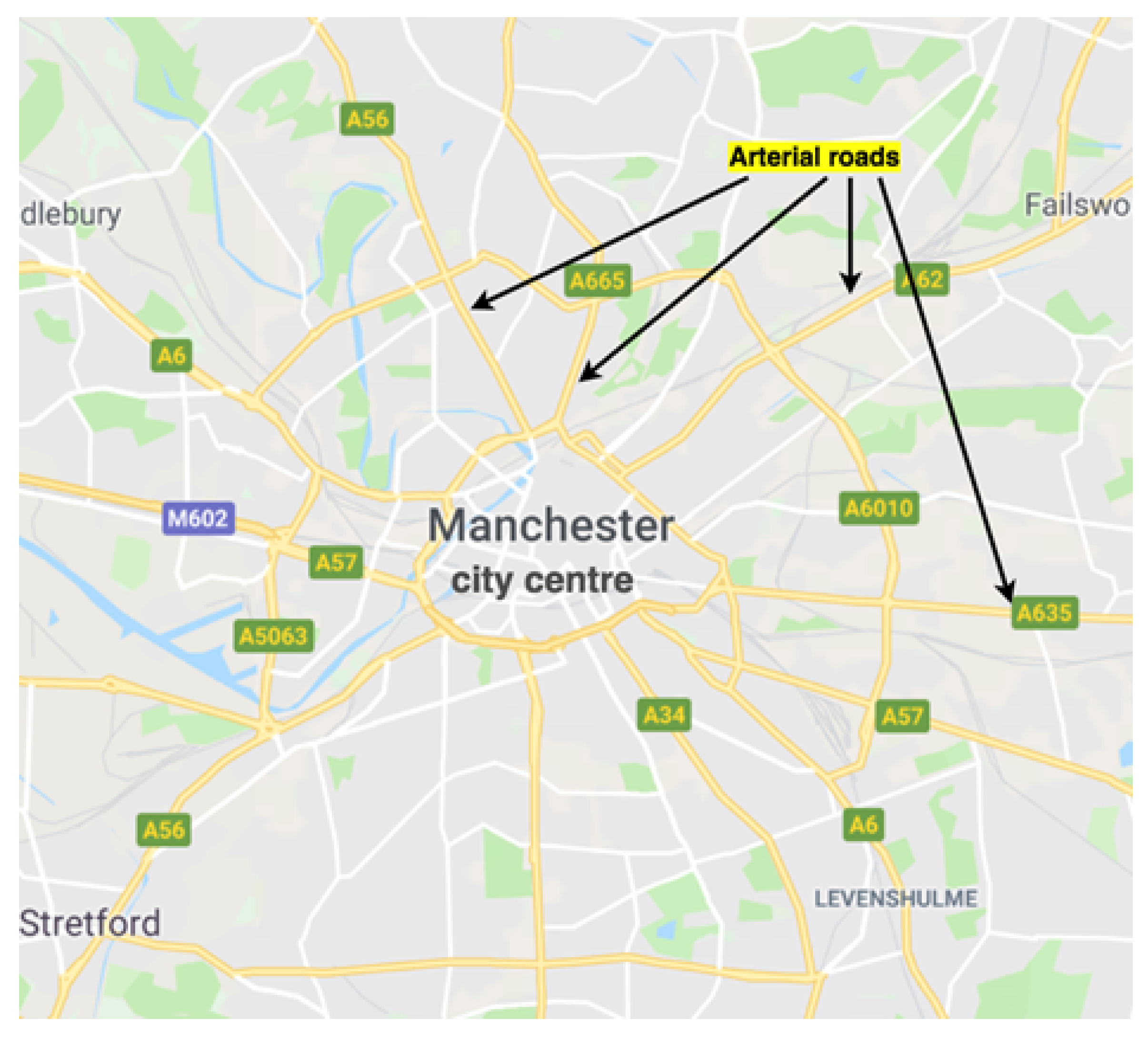
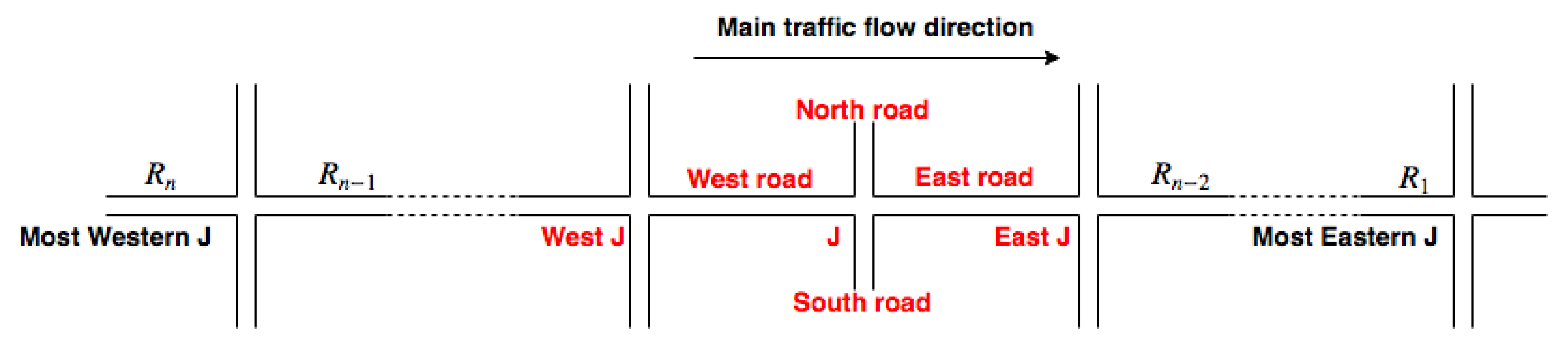
Figure 1 shows the map of the city of Manchester and highlights some arterial roads along with the location of the city centre. A simplified version of an arterial road is illustrated in Figure 2 where the main traffic flow direction indicates the prioritized direction (used by vehicles to exit the city centre). The labels in red are the description of roads and junctions relative to the junction J (in the centre). These terminologies will be used throughout the rest of this paper.
3.1. Sensors Deployment on Road Networks
One of the main requirements for the successful deployment of an efficient ATLCS is the accurate estimation of the number of vehicles on the roads. There are many ways this could be achieved, such as using inductive loops, magnetic sensors, magnetometers or even cameras. Reference [13] provides an overview of the different traffic sensing technologies and after examination of their respective advantages and drawbacks, we have chosen the magnetometer sensors as the main sensing technology to be deployed in our system. These sensors are able to detect the presence of vehicles that pass over them by detecting the change in the Earth’s magnetic field. They show several salient features, such as being easily powered by batteries, and their performance does not deteriorate under bad weather conditions. They can also perform simple computations, save and transmit the sensed data over a radio frequency. Moreover, their performance is not affected by the pressure created by vehicles when passing on top of them. It is worth mentioning that they have a few disadvantages such as the requirement to cut pavements during their installation and the need for a road closure for maintenance.
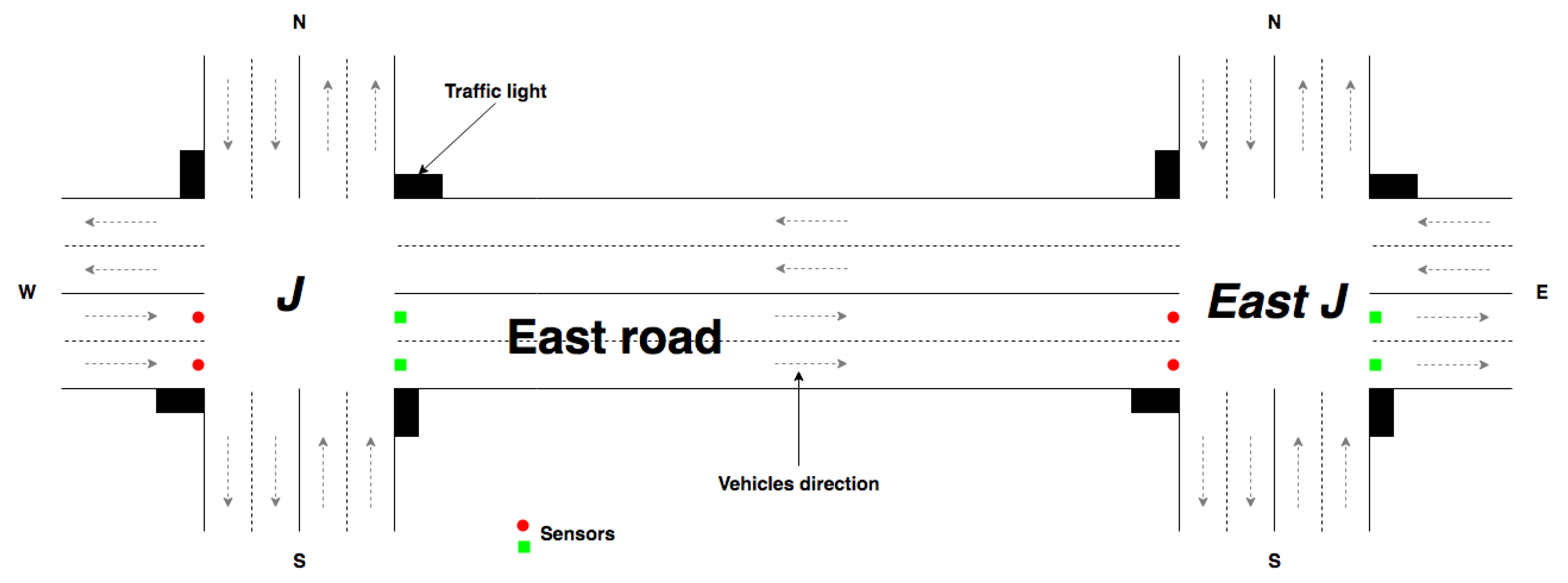
In this paper, we will only consider 2-lane roads, hence the road networks architecture adopted requires four sensors per junction as illustrated in Figure 3, which depicts the deployed sensors locations in two adjacent arterial junctions. We can see that the red sensors detect vehicles coming from the West and going toward the junction whereas the green sensors detect vehicles leaving the junction and moving toward the East. The number of vehicles on the road between two adjacent junctions (East road relative to junction J) is the difference between the number of vehicles that have passed over the green sensors of the junction J and the number of vehicles that have passed over the red sensors of the East junction.
3.2. Traffic Light Controller Synchronization Algorithm
All Traffic Lights (TLs) use a cycle of 8 different phases as illustrated in Figure 4. In this figure, the green curves show the allowed vehicle movements and the amber ones signal the end of the last phase. Forbidden movements (red signal) are not displayed for simplicity purposes. Only vehicle movements heading to the East road are represented to keep the figure clear. This cycle is the one commonly used in traffic light controllers in main roads because it minimizes the risk of collision while allowing any possible movement.
In the following, we will describe how the traffic lights controller synchronization is achieved in one direction (from West to East).
3.2.1. Computing the Position and Velocity of a Vehicle
The following equations represent the evolution of vehicles’ speed over time if we assume that vehicles move at a constant acceleration a until they reach the road speed limit from which point they drive at that constant speed.
where denotes the time when the vehicle reaches the speed and the initial velocity. We can infer from Equation (1) that:
Following the law of physics, the equation describing the position of the vehicle can be obtained by integrating the velocity expression over the time:
3.2.2. Representing a Queue of Vehicles
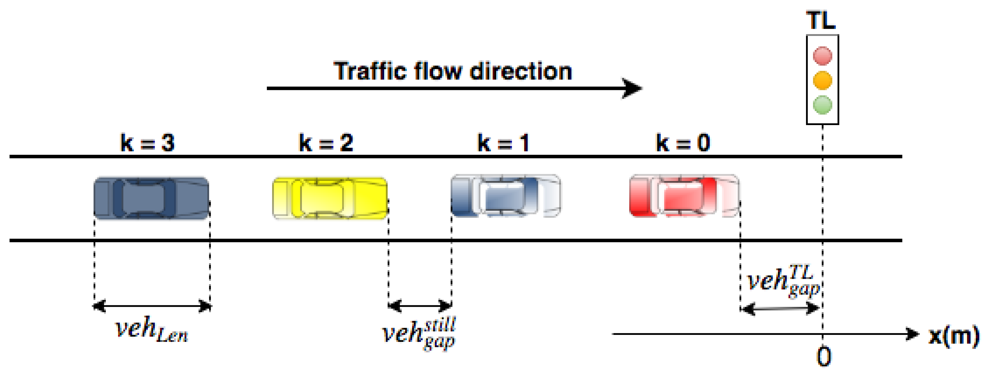
If we consider a queue of stationary vehicles () waiting at the traffic light as illustrated in Figure 5, the position of the kth vehicle in the queue, given that the first vehicle is at position 0, the second vehicle at position 1, etc., is described by the following equations:
where
and
where
- represents the average length of vehicles.
- refers to the gap between two stationary vehicles (one behind the other) in the queue.
- denotes the gap between the vehicle at the head of the queue and the TL location.
- defines the interval between the time at which a vehicle in the queue starts moving and the vehicle right behind it.
- refers to the time when the vehicle at the position k starts moving.
- denotes the time when the vehicle at the position k reaches the speed .
The velocity can be obtained by computing the derivative of the position as follows.
which gives the following result:
3.2.3. Adjacent Junctions Synchronization
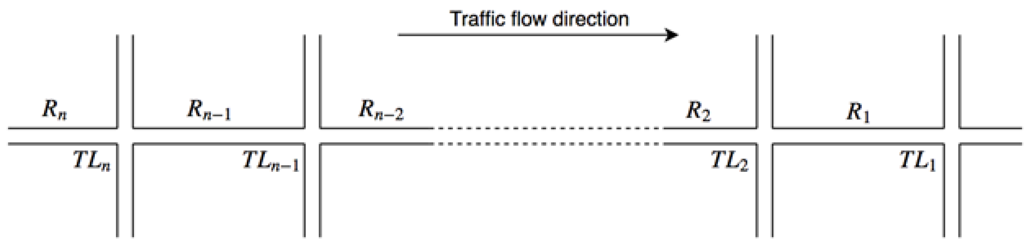
This section describes how synchronization between two adjacent TLs is achieved. Let us consider a road network with n junctions (, , …, ) as illustrated in Figure 6. is the most Eastern traffic light and is the most Western one. The TLs are all linked together by n − 1 road segments (, , …, ), with being the road segment between and .
Synchronization: Two-Way Roads with a Single Lane
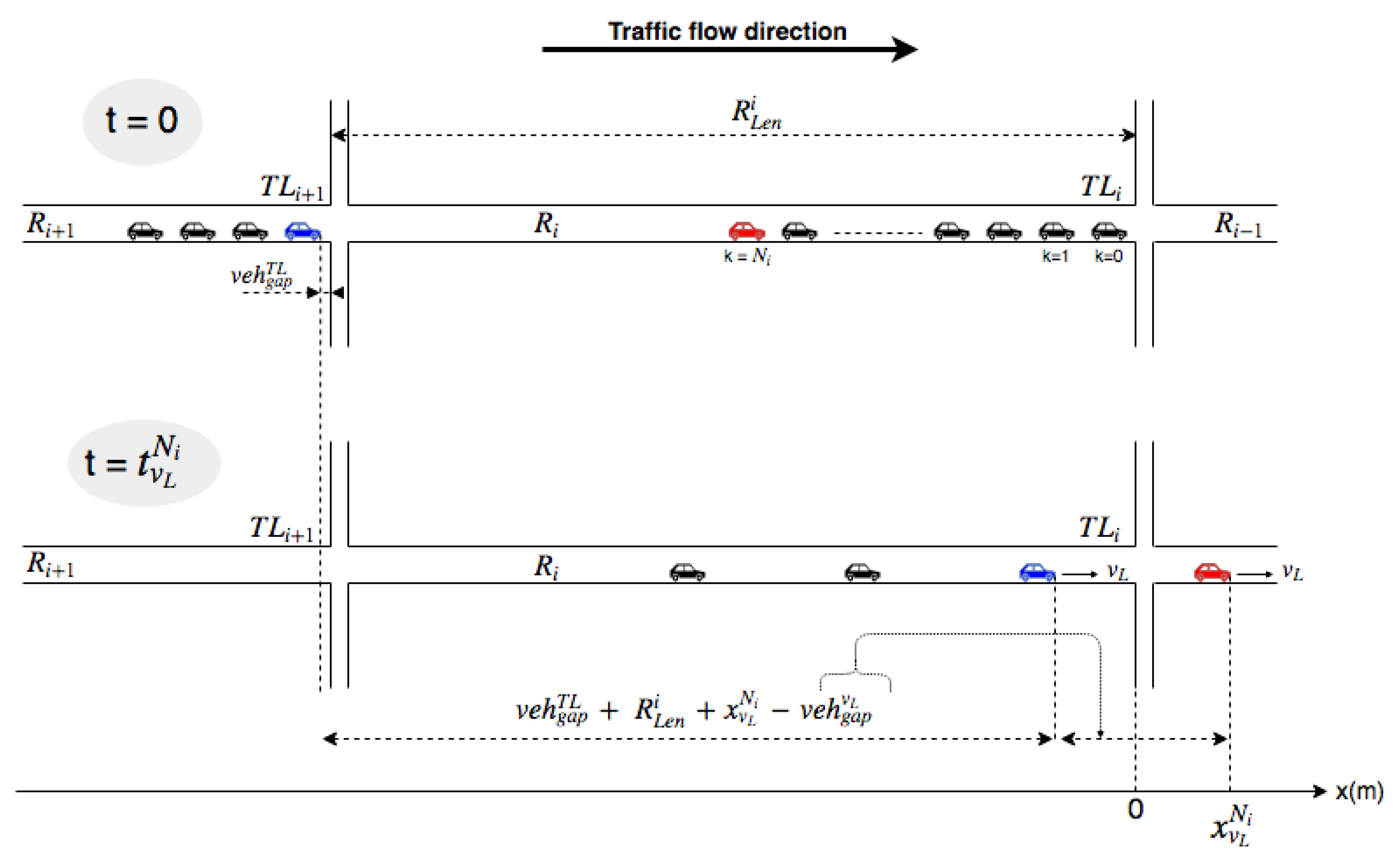
For simplicity purposes, we consider a set of two way roads with a single lane in each direction. We assume that and are both red (phase 8) on the traffic flow direction shown in Figure 7 with stationary vehicles queued up on the roads and . When switches to green, is considered to be synchronized with it if the blue vehicle (at the head of the queue in ) reaches the red vehicle (at the end of the queue in ) while both are traveling at the same speed. Assuming that the road is clear ahead, the speed for both vehicles to meet up should be the road speed limit .
From Equations (11)–(13) and (18) we can compute the time and the distance traveled when the red vehicle reaches , as follows:
By substituting Equation (20) in Equation (19) we get:
with being the number of vehicles in the queue on .
Figure 7 illustrates two snapshots of two adjacent junctions of a road network. The top figure shows the road network state at the time when switches to green (i.e., ) whereas the figure at the bottom illustrates vehicles positions and speed at the time . This is the time when the red vehicle reaches the speed limit . From Equation (21) we know that the red vehicle is located at the position . This is not the distance traveled but rather the position in the x-axis as shown in Figure 7. The blue vehicle needs to reach the red one while traveling at a speed of leaving a gap of between the two of them. The gap mentioned here is the distance between the front of the vehicle ahead and the front of the vehicle behind. This gap can intuitively be retrieved from the knowledge of the initial gap when both vehicles are stationary , the length of the vehicles and the interval between the time when each vehicle starts moving :
From Figure 7, we can see that the distance the blue vehicle needs to travel to reach the red vehicle is:
where represents the length of the road . By substituting the equations Equations (20), (22) and (23) in Equation (21) and then both Equations (21) and (24) in Equation (25) we obtain the following:
By substituting Equation (26) in Equation (10) and solving the resulting equation for k = 0 (head of the queue), we obtain the time required by the blue vehicle to meet the red one, expressed as follows:
This means that should switch to green (i.e., phase 1) seconds after for both TLs to be synchronized.
with
where refers to the time at which and are synchronized. By substituting Equation (23) in Equation (20) and then Equations (20) and (28) in Equation (30) we get:
with being the number of vehicles in the queue on .
Synchronization: Two-Way Roads with Multiple Lanes
Now, we focus on how adjacent TLs synchronization can be achieved on road networks with multiple lanes (i.e., more than one lane in each direction). For the sake of simplicity we assume that all roads have the same number of lanes. From the location of sensors described previously, we know that the total number of vehicles on any arterial road can be retrieved from the sensor counts. The number of vehicles on each lane is, however, unknown. We will, therefore, assume that the number of vehicles on the road is equally distributed over all lanes. As a future work, if Connected and Autonomous Vehicles technology is considered then the last vehicle in the queue of each lane will notify the TL about its current position so that more accurate synchronization can be achieved. With this assumption, multiple lanes synchronization problem could be reduced to a single lane by using the average number of vehicles per lane in the queue, as described below.
3.2.4. Multiple Junctions Synchronization
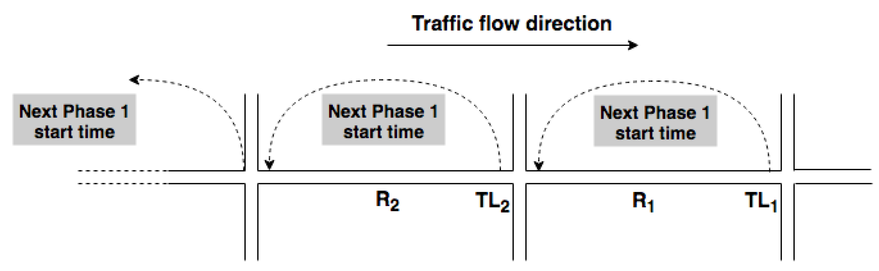
In the previous section, we have shown how two adjacent TLs can be synchronized. This section will build on that development and show how synchronization on a road with multiple junctions is achieved. When there are multiple junctions on the road, the synchronization across the road is done by synchronizing two adjacent TLs in cascade starting from the most Eastern ones. As shown in Figure 8, which leads the synchronization process signals to its next phase 1 start time before reaching it. From the moment receives that information, it computes its next phase 1 time to synchronize with . At the time knows when it will switch to phase 1 in the next cycle, it communicates that information to which in return does the same thing. This process is continued until the most Western TL is reached.
From the 8 phases in the TL cycle described previously (see Figure 4, the duration of the phases 2 till 8 will be fixed for all TLs. The phase 1 duration of all TLs with the exception of will be adjusted dynamically in order to synchronize with their respective East junction. The phase 1 duration for will be fixed () because it is the first TL and, therefore, does not synchronize with any other TL.
The flowchart in Figure 9 describes the different steps of our synchronization algorithm. In the beginning, we consider that all TLs are in phase 1. will switch to phase 2 after seconds (its phase 1 duration). At the moment it switches to phase 2, it computes its next phase 1 start time () and sends it to . Notice that when the time of one specific phase is mentioned, it will always refer to the start time of that phase.
The moment a TLC (Traffic Light Controller) controlling any junction among (, …, ) receives the next phase 1 start time of its corresponding East TLC (i.e., ), it will still be in phase 1. It needs to find out its next phase 1 start time () to synchronize with the East junction during the next cycle. Determining the next phase 1 start time is exactly the same as finding out when to switch to phase 2 () or end the current phase 1 because the duration of phases 2 to 8 is fixed.
This means that we need to decide in advance when to switch to phase 2 in order to synchronize with East TL. From Equation (31), we know the time delay between the start of both TLs (current TL and the East one) phase 1 required to achieve the sought synchronization.
Now, the only unknown parameter to find is the number of vehicles in the East road at the start of the next phase 1 of the East junction, expressed as
Because the current TL is still in phase 1, the only option to know the number of vehicles in the East road in the near future is to estimate it. If we consider that the current TL switches to phase 2 now, the number of vehicles in the East road at the time can be estimated by summing the current number of vehicles in the East road and the number of vehicles that came from the North and South roads and went to the East road during the last cycle as described in the Equation (37).
This is why, during every cycle, all TLCs with the exception of count the number of vehicles that pass over their green sensors from the start of phase 5 until the end of phase 8. From the phase cycle described in Figure 4, we can see that this count number represents the number of vehicles that come from the North and South roads and go to the East road .
The computation of the start time of phase 2 that would lead to synchronization is shown below:
or
The process of determining when a TL switches to phase 2, however, is done every second because during the current phase 1 the number of vehicles in the East road keeps increasing which causes the computed switching time () to change over time. Switching to phase 2 is triggered whenever the current time (t) is equal or greater than the time computed to switch (i.e., ). Once the switch operation is completed, the TLC sends to its corresponding West TLC the next time it will switch to phase 1, as computed in Equation (33).
4. Performance Evaluation
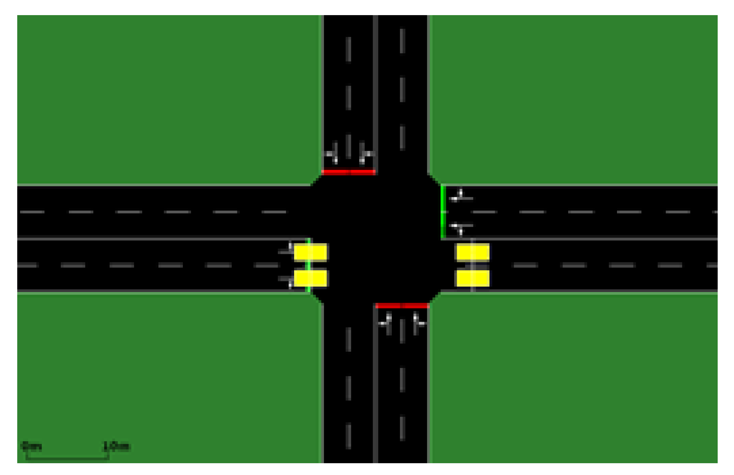
Our proposed ATLCS has been implemented in Python using SUMO (Simulation of Urban Mobility) and TraCI (Traffic Control Interface) packages [14]. Its performance evaluation is carried out using a road network with 4 main junctions joined together by 3 equal length road segments as illustrated in Figure 10. The location of sensors (yellow rectangles) is illustrated in Figure 11.
Table 1 summarizes the simulation setting in terms of vehicles and road network parameters whereas Table 2 lists the TLCs phases duration. The results presented are the average of 50 different simulations and the duration of each simulation lasts about 26 min of real-time road traffic. The results presented below are for vehicles traveling from West to East (prioritized direction) unless explicitly expressed otherwise.
The simulation is performed by initializing the TLs randomly (the first phase and its offset are both random). The simulation is run 50 times and the average of these results are used to illustrate how our synchronized ATLCS performs compared to a fixed time TLCS (i.e., without synchronization), where the phase 1 duration is set to . The evaluation is done using different metrics such as the Average Travel Time (ATT) and the Travel Time Index (TTI). The ATT is the average time taken by vehicles in the network to complete their predetermined route and the TTI is the ratio between the current ATT and the free flow travel time. Simulations will be performed using three different values of (1 min, 2 min and 3 min) where is the phase 1 duration for the first traffic light (). It also represents the phase 1 duration of all TLCs for the fixed time TLCS (non-synchronized).
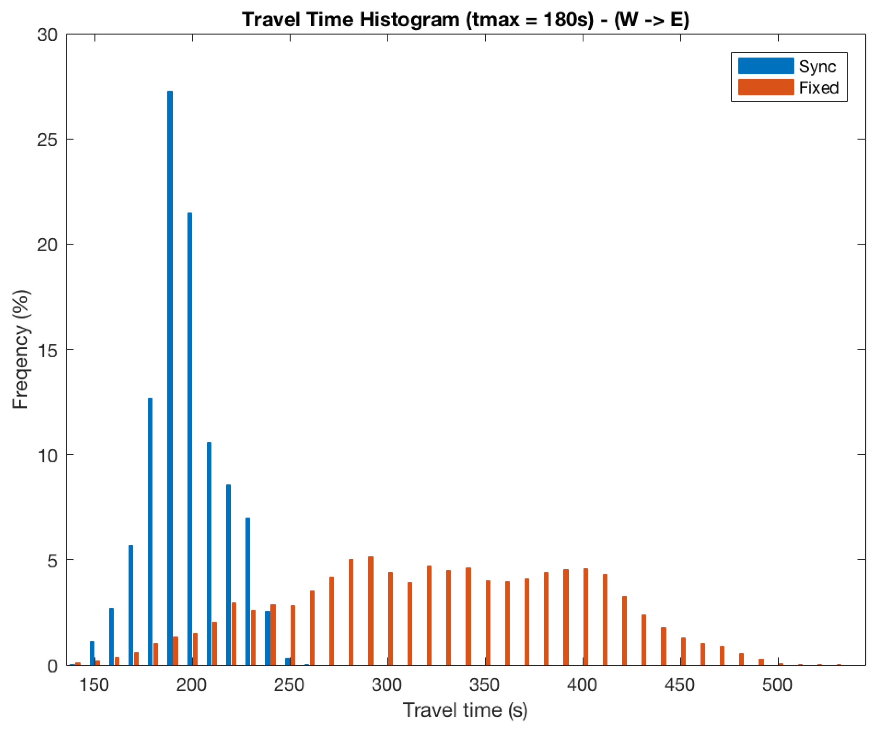
Figure 12 depicts the variation of the achieved trips duration (i.e., travel time) in fixed and synchronized TLCSs. The results shown are grouped by 10 s interval for a value equals to 3 min. We can observe that our synchronized ATLCS has much higher number of shorter trips (lower than 250 s) compared to the fixed time TLCS which has a significantly higher number of longer trips (up to 500 s). This is due to the fact that the synchronization process at arterial roads allows a large portion of vehicles to reach their destination with lower number of stops (i.e., a reduction in the ‘stop and go’ phenomenon), hence the faster progress towards their destinations.
Figure 13 shows the travel time achieved per simulation for = 3 min. The dot in the middle of the vertical lines represents the ATT per simulation whereas the line at the top and bottom of the vertical lines represent the maximum and minimum travel time for each simulation. We can see that for our synchronized ATLCS (in blue) the average, minimum and maximum values of the travel time are almost the same (minor variation observed only) for all simulations whereas the values for the non-synchronized fixed time TLCS vary a lot across the different simulation runs. The reason behind such variation is the lack of synchronization as well as the varying number of vehicles queued behind the TL, at each simulation run, leading to a significant variation in the number of stoppages, avoided in our ATLCS, and thus the increase in travel time.
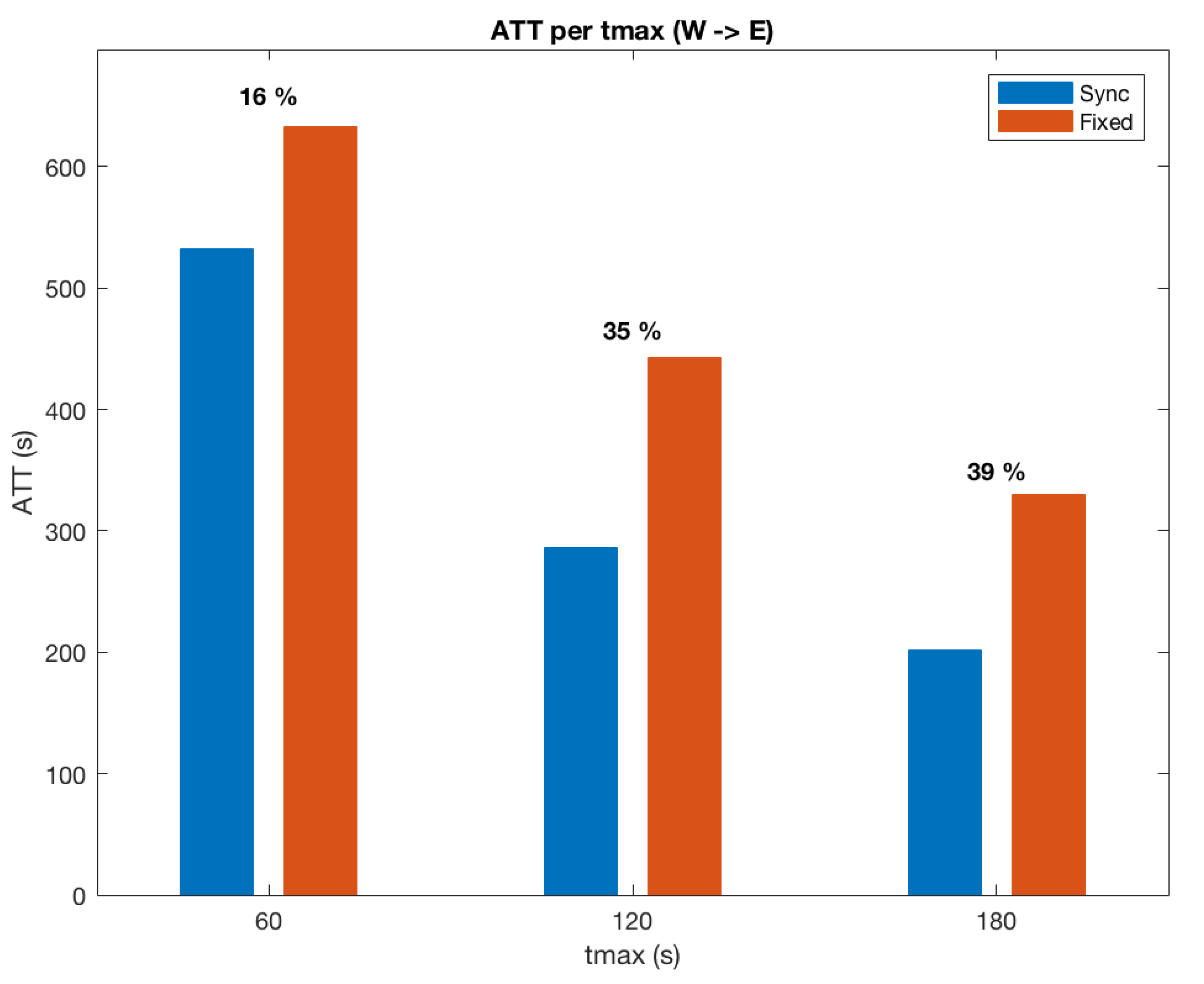
Figure 14 illustrates the impact of the value on the achieved ATT. The percentage values on top of the bars represent the improvement achieved by the synchronized ATLS compared to the non-synchronized fixed time TLCS. We observe that the highest improvement (39%) is achieved for a value of 3 min. Notice that the substantial benefit of the synchronization is achieved for higher values of because this allows a large number of vehicles to travel a long distance without having to stop as the green wave lasts for a longer period compared the scenarios when is set to 1 and 2 min.
All the results discussed so far were for a highly congested road network (i.e., the road is used to its full capacity). Figure 15 shows the ATT achieved for different levels of road network occupancy. A road network occupancy level of 100% means that the rate at which new vehicles are added to the road network is the maximum (about 1 vehicle every 2.4 s per lane). This should be interpreted as a highly congested road network. The highest improvement (39%) occurs when the road network occupancy level is maximal.
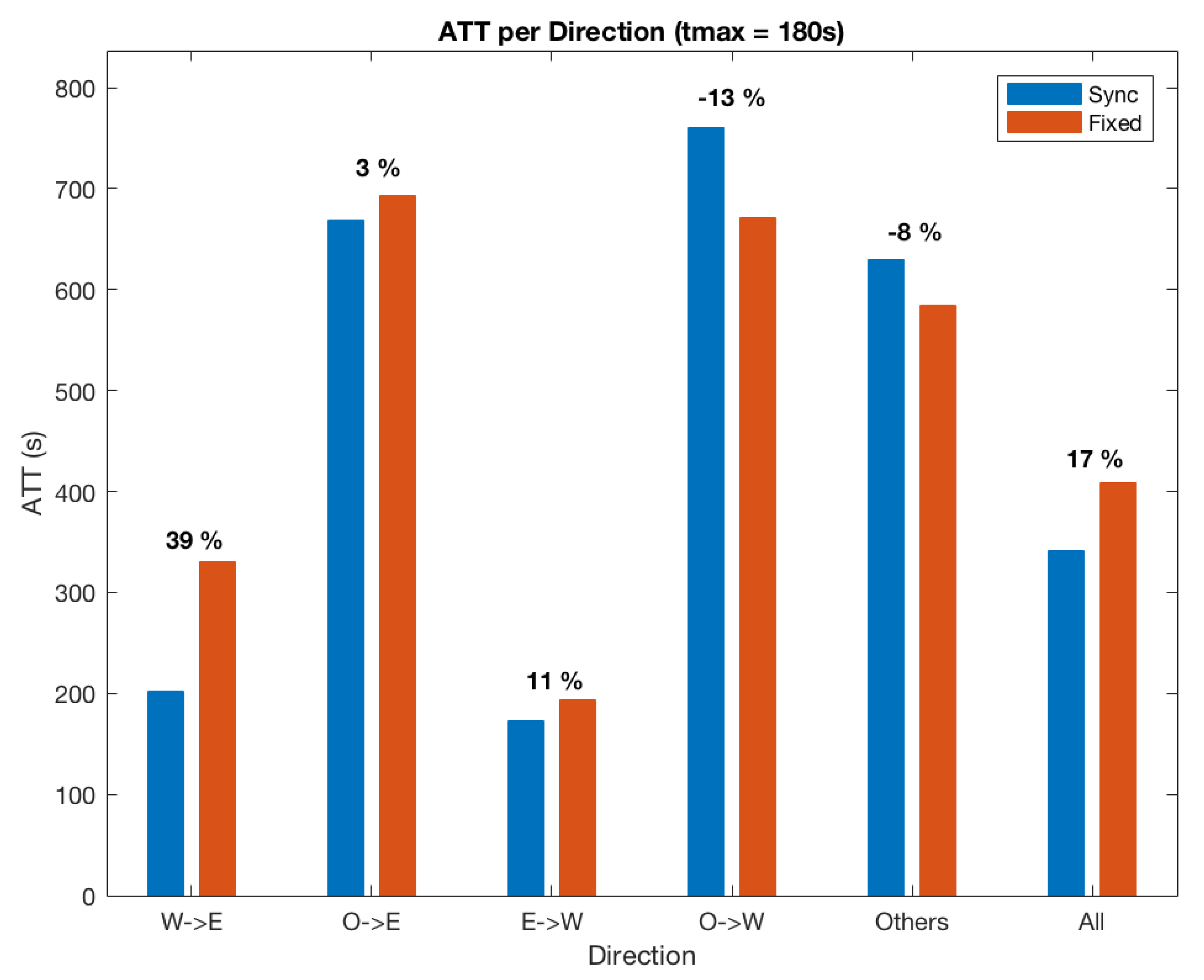
All the results presented so far have only considered vehicles traveling on the arterial road from the West to the East while ignoring the vehicles traveling on other directions. This is because this solution aims primarily at reducing the congestion level in the city centre by maximizing the number of vehicles leaving it (West to East). Figure 16 depicts the ATT achieved for vehicles traveling in other directions. The description of all direction labels in Figure 16 is summarized as follows: W->E means West to East, O->E means Other than West to East, E->W means East to West, O->W means Other than East to West, Others means From/To North or South, and All refers to All directions. We can see that the ATT improvement could be positive or negative depending on the direction considered. The overall ATT improvement, when all vehicles in the network are taken into consideration, is 17%. There is also an improvement of 11% for vehicles traveling in the opposite direction of the prioritized one (East to West). From these results we can conclude that our proposed synchronized ATLCS does not only lead to significant enhancement of the ATT of the vehicles traveling on the prioritized direction but also yields an important decrease of the travel time across the whole network.
In addition to the ATT we have also measured the achieved Travel Time Index (TTI). TTI is the ratio of the TT during peak hours compared to the free flow TT which refers to the time needed for a vehicle to cross a road during optimal conditions, i.e., at the maximum allowed speed with no delays [15]. TTI is a useful metric for assessing the congestion level in road networks, it is computed as follows.
The free flow traffic time is 139s. It has been determined by setting all TLCs to phase 1 and getting the travel time of vehicles traveling from West to East. For = 3 min and a road network occupancy level of 100%, the TTI of vehicles traveling from West to East for our synchronized ATLS and the fixed time TLCS are:
and
From Equations (42) and (43) we infer that our synchronized ATLCS outperforms the fixed time TLCS since the former achieves a higher value of TTI, meaning that it successfully reduces the impact of congestion, compared to the latter (an improvement of 63%) because the higher the TTI is the faster traffic will be.
5. Conclusions
A novel efficient Adaptive Traffic Light Control System (ATLCS) has been proposed to aid traffic management authorities in dealing with the road traffic congestion problem and its resulting impact on journey times, road safety, air quality and the economy. The evaluation results of our proposed synchronization algorithm have shown an important decrease in the average travel time for vehicles crossing intersections controlled by the synchronized TLCSs. Despite these encouraging results, this work is yet to be completed, as a testing on real world scenarios would be the next logical step to confirm its effectiveness. Therefore, as a future work, we plan to collaborate with Traffic for Greater Manchester (TfGM), the authority managing the road network in the Greater Manchester area, in order to test our algorithm in their Traffic Light Control Systems.
Author Contributions
Conceptualization, D.R.A. and S.D.; methodology, D.R.A. and S.D.; software, D.R.A.; validation, D.R.A.; formal analysis, D.R.A. and S.D.; investigation, D.R.A. and S.D.; data curation, D.R.A.; writing—original draft preparation, D.R.A. and S.D.; writing—review and editing, S.D.; visualization, D.R.A.; supervision, S.D. All authors have read and agreed to the published version of the manuscript.
Funding
This research received no external funding.
Conflicts of Interest
The authors declare no conflict of interest.
References
- Djahel, S.; Doolan, R.; Muntean, G.; Murphy, J. A Communications-Oriented Perspective on Traffic Management Systems for Smart Cities: Challenges and Innovative Approaches. IEEE Commun. Surv. Tutor. 2014, 17, 125–151. [Google Scholar] [CrossRef]
- Barth, M.; Boriboonsomsin, K. Real-world carbon dioxide impacts of traffic congestion. Transp. Res. Rec. 2008, 2058, 163–171. [Google Scholar] [CrossRef] [Green Version]
- INRIX. Traffic Congestion Cost UK Motorists More Than £30 Billion in 2016. Available online: https://inrix.com/press-releases/traffic-congestion-cost-uk-motorists-more-than-30-billion-in-2016/ (accessed on 21 February 2020).
- Aleko, D.R.; Djahel, S. An IoT Enabled Traffic Light Controllers Synchronization Method for Road Traffic Congestion Mitigation. In Proceedings of the 2019 IEEE International Smart Cities Conference (IEEE ISC2), Casablanca, Morocco, 14–17 October 2019. [Google Scholar]
- Li, J.; Zhang, Y.; Chen, Y. A Self-Adaptive Traffic Light Control System Based on Speed of Vehicles. In Proceedings of the 2016 IEEE International Conference on Software Quality, Reliability and Security Companion (QRS-C), Vienna, Austria, 1–3 August 2016; pp. 382–388. [Google Scholar]
- Djahel, S.; Smith, N.; Wang, S.; Murphy, J. Reducing emergency services response time in smart cities: An advanced adaptive and fuzzy approach. In Proceedings of the 2015 IEEE First International Smart Cities Conference (ISC2), Guadalajara, Mexico, 25–28 October 2015; pp. 1–8. [Google Scholar]
- Faye, S.; Chaudet, C.; Demeure, I. A distributed algorithm for adaptive traffic lights control. In Proceedings of the 2012 15th International IEEE Conference on Intelligent Transportation Systems, Anchorage, AK, USA, 16–19 September 2012; pp. 1572–1577. [Google Scholar]
- Faye, F.; Chaudet, C.; Demeure, I. A distributed algorithm for multiple intersections adaptive traffic lights control using a wireless sensor networks. In First Workshop on Urban Networking (UrbaNe ’12); ACM: New York, NY, USA, 2012; pp. 13–18. [Google Scholar]
- Coll, P.; Factorovich, P.; Loiseau, I.; Gómez, R. A linear programming approach for adaptive synchronization of traffic signals. Int. Trans. Oper. Res. 2013, 20, 667–679. [Google Scholar] [CrossRef]
- García-Nieto, J.; Alba, E.; Olivera, A.C. Swarm intelligence for traffic light scheduling: Application to real urban areas. Appl. Artif. Intell. 2012, 25, 274–283. [Google Scholar] [CrossRef]
- Astarita, V.; Festa, D.C.; Giofrè, V.P. Cooperative-Competitive Paradigm in Traffic Signal Synchronization Based on Floating Car Data. In Proceedings of the 2018 IEEE International Conference on Environment and Electrical Engineering and 2018 IEEE Industrial and Commercial Power Systems Europe (EEEIC/I&CPS Europe), Palermo, Italy, 12–15 June 2018; pp. 1–6. [Google Scholar]
- Liu, J.; Li, J.; Zhang, L.; Dai, F.; Zhang, Y.; Meng, X.; Shen, J. Secure intelligent traffic light control using fog computing. Future Gener. Comput. Syst. 2018, 78, 817–824. [Google Scholar] [CrossRef]
- Nellore, K.; Hancke, G.P. A Survey on Urban Traffic Management System Using Wireless Sensor Networks. Sensors 2016, 16, 157. [Google Scholar] [CrossRef] [Green Version]
- Behrisch, M.; Bieker, L.; Erdmann, J.; Krajzewicz, D. SUMO—Simulation of Urban MObility: An Overview. In Proceedings of SIMUL 2011, The Third International Conference on Advances in System Simulation; ThinkMind: Barcelona, Spain, 2011. [Google Scholar]
- Schrank, D.; Eisele, B.; Lomax, T. TTI’s 2012 Urban Mobility Report; Texas A&M Transportation Institute, The Texas A&M University System: College Station, TX, USA, 2012. [Google Scholar]
Figure 1.
Manchester city arterial roads.

Figure 2.
Example of an arterial road with multiple junctions.

Figure 3.
Illustration of sensors deployment on adjacent arterial junctions.

Figure 4.
Phases of the traffic lights cycle (only movements from West to East are displayed).

Figure 5.
Queue of vehicles behind a Traffic Light (TL).

Figure 6.
Adjacent junctions in a road network.

Figure 7.
Illustration of adjacent traffic lights synchronization mechanism.

Figure 8.
Multiple junctions synchronization process.

Figure 9.
Illustration of TLs synchronization steps.

Figure 10.
An arterial road with 4 junctions.

Figure 11.
Arterial junction with sensor locations (yellow rectangle).

Figure 12.
Travel time distribution: fixed time Traffic Light Control System (TLCS) vs. synchronized Adaptive Traffic Light Control System (ATLCS).
Figure 12.
Travel time distribution: fixed time Traffic Light Control System (TLCS) vs. synchronized Adaptive Traffic Light Control System (ATLCS).

Figure 13.
Travel time variation over different simulation runs: fixed time TLCS vs. synchronized ATLCS.
Figure 13.
Travel time variation over different simulation runs: fixed time TLCS vs. synchronized ATLCS.

Figure 14.
Impact of value on the achieved Average Travel Time (ATT).

Figure 15.
Impact of road network occupancy on the achieved ATT.

Figure 16.
The achieved ATT in different travel directions.


Table 1.
Vehicles and road network parameters.
| Parameter | Value |
|---|---|
| Road length | 300 m |
| Congestion level | Maximum or 100% |
| Vehicle length | 4.3 m |
| Gap between vehicles in queue | 2.5 m |
| Road speed limit | 13.89 m/s–31.07 mph-5-0 km/h |
| Gap between the 1st vehicle | 1 m |
| and TL in queue | |
| Delay between the start of 2 | 1 s |
| consecutive vehicles in a queue | |
| Vehicle acceleration | 2.9 m/s |
Table 2.
TL cycle phases duration.
| Phase | Duration |
|---|---|
| 1 | 240 s (only for TL1) |
| 2-4-6-8 | 4 s |
| 3-7 | 6 s |
| 5 | 31 s |
© 2020 by the authors. Licensee MDPI, Basel, Switzerland. This article is an open access article distributed under the terms and conditions of the Creative Commons Attribution (CC BY) license (http://creativecommons.org/licenses/by/4.0/).
Share and Cite
MDPI and ACS Style
ALEKO, D.R.; Djahel, S. An Efficient Adaptive Traffic Light Control System for Urban Road Traffic Congestion Reduction in Smart Cities. Information 2020, 11, 119. https://0-doi-org.brum.beds.ac.uk/10.3390/info11020119
AMA Style
ALEKO DR, Djahel S. An Efficient Adaptive Traffic Light Control System for Urban Road Traffic Congestion Reduction in Smart Cities. Information. 2020; 11(2):119. https://0-doi-org.brum.beds.ac.uk/10.3390/info11020119
Chicago/Turabian StyleALEKO, Dex R., and Soufiene Djahel. 2020. "An Efficient Adaptive Traffic Light Control System for Urban Road Traffic Congestion Reduction in Smart Cities" Information 11, no. 2: 119. https://0-doi-org.brum.beds.ac.uk/10.3390/info11020119
Note that from the first issue of 2016, this journal uses article numbers instead of page numbers. See further details here.