Model for Collaboration among Carriers to Reduce Empty Container Truck Trips †


1
National Transportation Research Center, Oak Ridge National Laboratory, Knoxville, TN 37932, USA
2
Department of Civil and Environmental Engineering, University of South Carolina, Columbia, SC 29208, USA
*
Author to whom correspondence should be addressed.
†
This manuscript has been authored by UT-Battelle, LLC, under contract DE-AC05-00OR22725 with the US Department of Energy (DOE). The US government retains and the publisher, by accepting the article for publication, acknowledges that the US government retains a nonexclusive, paid-up, irrevocable, worldwide license to publish or reproduce the published form of this manuscript, or allow others to do so, for US government purposes. DOE will provide public access to these results of federally sponsored research in accordance with the DOE Public Access Plan (http://energy.gov/downloads/doe-public-access-plan ).
Information 2020, 11(8), 377; https://0-doi-org.brum.beds.ac.uk/10.3390/info11080377
Submission received: 18 May 2020
/
Revised: 23 July 2020
/
Accepted: 24 July 2020
/
Published: 26 July 2020
(This article belongs to the Special Issue Modeling of Supply Chain Systems)
Abstract
:In recent years, intermodal transport has become an increasingly attractive alternative to freight shippers. However, the current intermodal freight transport is not as efficient as it could be. Oftentimes an empty container needs to be transported from the empty container depot to the shipper, and conversely, an empty container needs to be transported from the receiver to the empty container depot. These empty container movements decrease the freight carrier’s profit, as well as increase traffic congestion, decrease roadway safety, and add unnecessary emissions to the environment. To this end, our study evaluates a potential collaboration strategy to be used by carriers for domestic intermodal freight transport based on an optimization approach to reduce the number of empty container trips. A binary integer-linear programming model is developed to determine each freight carrier’s optimal schedule while minimizing its operating cost. The model ensures that the cost for each carrier with collaboration is less than or equal to its cost without collaboration. It also ensures that average savings from the collaboration are shared equally among all participating carriers. Additionally, two stochastic models are provided to account for uncertainty in truck travel times. The proposed collaboration strategy is tested using empirical data and is demonstrated to be effective in meeting all of the shipment constraints.
1. Introduction
Freight can be transported using a single mode or several modes. When more than one mode is used and no handling of freight is required for changing modes, it is known as intermodal. Intermodal freight transport provides several essential benefits for shippers due to the use of standard container sizes: faster transshipments, reduced packaging expenses and lower shipping costs [1,2]. Additionally, it offers an alternative to the highway mode to help reduce highway congestion, improve traffic safety and lower emissions. Due to the aforementioned advantages, intermodal transport has become an increasingly attractive alternative to freight shippers in recent years. For example, in 2019 the U.S. freight network moved about 18 million intermodal containers, which represents an increase of about 12.5% over the previous 5 years [3]. This trend is likely to continue as state and federal agencies seek to implement policies to induce a freight modal shift from road to intermodal transport.
Given the high volume and rapid growth, domestic intermodal transport needs to be efficient. However, the current intermodal freight transport is not as efficient as it could be. Oftentimes, an empty container needs to be transported from the empty container depot to the shipper, and conversely, an empty container needs to be transported from the receiver to the empty container depot. These empty container movements decrease the freight carrier’s profit, as well as add negative externalities to the environment (i.e., increased traffic congestion, increased traffic accident frequency and injury severity, and increased emissions). These issues are more pronounced in areas surrounding seaports or intermodal terminals/yards [4,5]. Therefore, a reduction in the number of empty container trips could help make intermodal freight transport more efficient and cost-effective.
This study aims to evaluate a potential collaboration strategy for domestic intermodal freight carriers based on an optimization approach to reduce the number of empty container trips such that it would benefit the participating freight carriers economically and the general public. Note that the proposed model does not include any specific aspect of intermodal freight transport, and thus can be applied to other freight transport areas such as less-than-truckload pickup and delivery problems. As defined by Caballini et al. [4], collaboration is the sharing of shipments among freight carriers to maximize their total profit (i.e., minimize their total operating cost). A major barrier in the implementation of collaboration is the issue of sharing customer information with competing carriers. That is, for business reasons, some carriers will not want their competitors to know who their clients/customers are. However, it is anticipated that the benefit of collaboration will outweigh the risk. This is similar to how most consumers continue to use credit cards, shop and pay for things online, and have “smart” devices in their homes even though all of these activities and devices pose a security risk.
In this study, it is assumed that when freight carriers collaborate, they are specifically looking to reduce empty container truck trips. This can be accomplished either by combining an inbound with an outbound shipment or by making a horizontal street-turn or vertical street-turn. The objective of the proposed model is to optimally combine inbound and outbound shipments in order to minimize the total operating cost incurred by the carriers. The model also ensures that the average savings (i.e., cost reduction under collaboration) for all carriers are shared equally. This profit-sharing scheme, which is common in freight supply chain collaboration [6,7], guarantees a financial benefit for each participating carrier. Additionally, stochastic versions of the model are proposed to consider uncertainty in truck travel times. This uncertainty consideration is essential for intermodal freight carriers to provide a reliable and on-time service to customers [8,9,10]. The experimental results, using the developed models and instances based on empirical data, demonstrate the effectiveness of collaboration in reducing the number of empty container trips and lowering costs for the participating carriers.
2. Literature Review
Collaborative logistics entails freight stakeholders working together to improve efficiency in their supply chains rather than operating in isolation. There are two forms of collaboration: vertical and horizontal collaboration. Vertical collaboration involves collaboration among stakeholders at different levels within a supply chain. It occurs when two or more organizations such as the manufacturer, the distributor, the carrier and the retailer share their responsibilities, resources and performance information in a way that improves efficiency [11]. On the other hand, horizontal collaboration involves collaboration between stakeholders at the same level of the supply chain. It occurs when two or more companies combine their resources to gain greater efficiency [12]. Given the scope of this study, a brief review of freight-related studies that explored the use of horizontal collaboration is provided. Readers are referred to review papers by Guajardo and Rönnqvist [6] and Gansterer and Hartl [13] for information regarding profit-sharing and cost allocation methods, and a review paper by Liu et al. [14] for information on empty container repositioning.
Horizontal collaborations have been studied for shippers [15,16,17,18] and carriers [4,5,7,19,20,21,22,23,24,25,26,27,28]. The main goal of collaboration among shippers is to negotiate better rates with the carriers, while the goal of collaboration among carriers is to reduce costs and compete with larger carriers. As for solution methodology, various methods such as optimization [4,5,7,15,16,17,18,19,20,22,23,24,25,26,27], game theory [7,15,17,19] and simulation [21,23,28] have been used. Optimization and game theory approaches have also been used successfully to solve different planning problems in intermodal transport (e.g., [29,30]). Cruijssen et al. [12] explored the potential benefits and impediments of horizontal collaboration using a survey participated in by 1537 logistics service providers. It was reported that in general, logistics service providers believe that horizontal collaboration can increase their profitability or improve the quality of their services. As for impediments, the study found that finding a reliable party to lead the collaboration and constructing a fair profit allocation/sharing scheme is the most important. Krajewska et al. [7] studied the distribution of both costs and savings arising from the horizontal collaboration using cooperative game theory. They showed that the computation of Shapley value is sufficient for fair allocation of costs among carriers. Agarwal and Ergun [19] studied carrier alliances in liner shipping. They utilized concepts from inverse programming and game theory to guide the carriers towards an optimal collaboration strategy. It was reported that the mechanism is capable of forming sustainable alliances. Dai and Chen [23] proposed a multi-agent and auction-based framework for carrier collaboration in less-than-truckload transportation. The purpose of the carrier collaboration is to optimize the transportation operations by sharing transportation requests and available vehicles. Chan and Zhang [21] used simulation to evaluate the benefits of collaborative transportation management and to optimize delivery speed. They found that collaboration can significantly reduce the total cost and improve delivery level of service. Similarly, Islam et al. [28] utilized simulation to explore dynamic truck-sharing facility so that export containers can be assigned to available empty slots. Their model was shown to reduce the number of empty container trips and increase the capacity of container transport around the port area. Frisk et al. [22] studied how cost savings should be distributed among forest companies involved in collaboration based on economic models. Quintero-Araujo et al. [25] analyzed different collaboration scenarios involving integrated routing and facility-location decisions in road transportation.
Xue et al. [27] minimized the total costs by assuming that tractors can be separated from companion trailers and be assigned to new trips. They also considered a strategic alliance in sharing empty containers between shippers and receivers. It was reported that the strategy can reduce the total travel distance and the number of containers employed. Sterzik et al. [26] studied two main variants of the problem where the containers may or may not be shared within the seaport-hinterland transportation with the objective of minimizing the vehicles total operating time. The study showed the potential benefits of sharing empty containers and highlighted the importance of developing mechanisms which motivate the companies to collaborate. Caballini et al. [4] studied a similar problem. The authors proposed an optimization model for the collaborative planning of multiple truck carrier operations in a seaport environment in order to maximize the total profit derived from the collaboration. They provided a compensation mechanism to motivate carriers to share their trips. The approach was evaluated using real data sets from the Italian Port of Genoa. Schulte et al. [5] developed a truck appointment system with collaboration. The appointment system is an optimization model based on multiple traveling salesman problems with time windows which can leverage collaboration to reduce cost and empty truck emissions in port areas. The model was verified with a case study demonstrating that it can enable a collaborative truck appointment system. Los et al. [24] proposed a multi-agent system where carriers and customers can interact, and carriers can share information for vehicle routing under collaboration. Atasoy et al. [20] studied a pickup and delivery problem with time windows under collaboration using real-world data from a transportation platform provider. The model ensured that the profit of each carrier under collaboration is higher or equal to that of without collaboration.
Table 1 presents an overview of the aforementioned studies. While some of these have considered equal sharing of profit, none has considered equal sharing in conjunction with the determination of optimal shipment planning. To address this shortcoming, our study proposes a collaboration scheme, based on an optimization model, for freight carriers in domestic intermodal transport. This scheme can be used to improve intermodal freight transport efficiency and cost effectiveness. It is based on the one proposed by Caballini et al. [4], with several notable extensions and contributions. This study customizes the model proposed by Caballini et al. for domestic intermodal freight transport, extends the model proposed by Caballini et al. to provide a realistic profit sharing scheme where the average savings from collaboration are shared equally among participating carriers, and transforms the model proposed by Caballini et al. into a stochastic model that takes into consideration the variations in truck travel time due to congestion and/or accidents.
3. Intermodal Freight Transport Model with Collaboration
Intermodal freight transportation industry is highly competitive, and carriers need to be efficient. One way to increase efficiency is to collaborate with other carriers to reduce unnecessary trips. This study considers a set of carriers which need to complete a set of jobs, consisting of a pair of inbound and outbound shipments, via an intermodal terminal/yard. The proposed model aims to assist the carriers in optimally planning their shipments while minimizing operating cost. It is assumed that there is a neutral central authority that collects job information and provides optimal routing to each carrier. This approach is called “centralized” in the literature.
The proposed model considers intermodal freight transport where containers can be moved by any one of the carriers operating in the same geographic area. During the considered time horizon (e.g., a day), each carrier must fulfill a specific transportation demand consisting of a set of shipments. A container going out of a terminal/yard is referred to as inbound shipment and a container going into a terminal/yard is referred to as outbound shipment. Each carrier is characterized by a unit operating cost, owns a certain number of trucks, and has a certain number of inbound and outbound shipments to be served. Each shipment has an origin, a destination and a deadline.
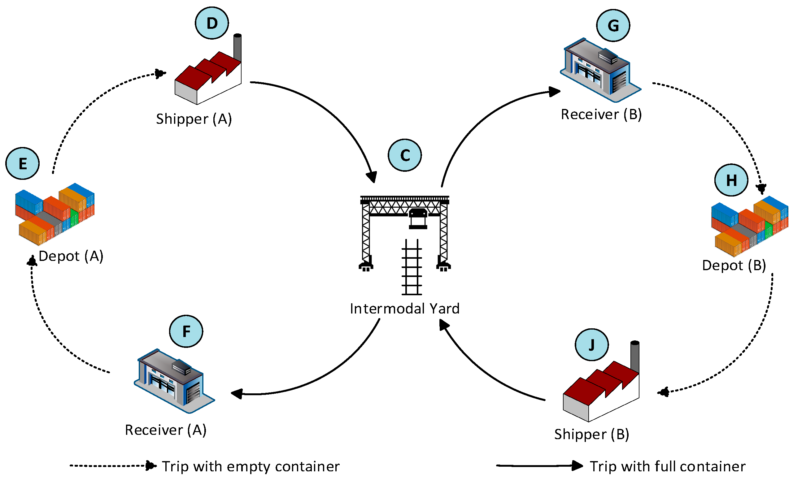
Figure 1 illustrates the intermodal freight transport process involving two freight carriers (carrier A and carrier B) that do not share shipments (i.e., without collaboration). For carrier A, a truck picks up an empty container from the empty container depot (E) and transport it to the shipper location (D) where the container is packed (outbound shipment). The truck then travels to the intermodal terminal/yard (C) with the full container. For an inbound shipment, a truck picks up the full container from the terminal/yard (C) and transports it to the receiver location (F) where the container is unpacked. The truck then travels to the empty container depot (E) with the empty container. Similar activities are performed by carrier B. As evident from this illustration, half of the truck trips consist of empty container movements.
Figure 2 illustrates the proposed shipment scheduling where freight carriers share shipments (i.e., with collaboration). For carrier A, instead of sending an empty container to the empty container depot from the receiver (F), it can send the empty container to its shipper (D) or to the shipper of another carrier (J). The first movement is referred to as “vertical street-turn” (VST) and the latter is referred to as “horizontal street-turn” (HST). Similarly, instead of sending an empty container to the empty container depot (H), carrier B can send the empty container to its shipper (J) or to the shipper of another carrier (D). Therefore, according to the above definitions, G to J is a VST trip and G to D is an HST trip. In this study, it is assumed that only one inbound and one outbound shipment can be combined under collaboration. Regarding the usage of containers, it is assumed that the freight carriers will use the same container for inbound and outbound shipments.
The intermodal freight transport network is represented by the graph . The set is the node set composed of (i) a subset of node representing the intermodal terminal/yard , (ii) the subset of shipper nodes , (iii) the subset of receiver nodes , and (iv) the subset of empty container depots , i.e., . The set represents the arcs connecting the nodes. It is assumed that the arcs are the shortest paths connecting each pair of nodes. The distance and travel time between the nodes are defined in Table 2. For example, the distance between shipper/receiver and the intermodal terminal/yard is defined as and the travel time is defined as . The distance between shipper/receiver and empty container depot is defined as and the travel time is defined as . The distance between shipper and receiver is defined as and the travel time is defined as . Lastly, the distance between empty container depots of the carriers is defined as and the travel time is defined as . Note that container (un)mount time is not considered since they are negligible compared to the travel times. The mathematical notations are summarized in Table 3.
As mentioned above, it is assumed that with carrier collaboration, only one inbound and one outbound shipment can be combined. Figure 3 shows the proposed time window framework for both single and combined (i.e., VST and HST) shipments. The middle part of the diagram shows the timing for shipment (inbound) and (outbound). For shipment , the finishing time must be less than or equal to the shipment deadline . The same is true for shipment . The lower part of the diagram shows the timing for the combined shipments. It is assumed that the first shipment () is delivered to meet its deadline. Depending on the travel time between customers’ locations (), the second shipment () may not meet its deadline . If the second shipment ends after its deadline , a penalty cost is incurred. The calculation of the penalty cost () is provided in Equation (1). Note that when the deadline for the second shipment is met, there is no penalty cost due to delay.
Based on the graph and notations defined above, an optimization model is formulated which minimizes the total operating cost of the collaborating freight carriers. The decision variables are as follows:
The operating cost of a carrier , , without collaboration can be calculated as follows:
The objective function of the proposed collaboration model (CM) is shown in Equation (5). The model outputs single and combined shipments to be performed by each carrier.
Subject to
The CM model is formulated as a binary integer-linear programming problem. The objective function in (5) minimizes the total operating cost of all freight carriers. Constraints (6) define the final operating cost for each carrier using single and combined shipments. Constraints (7) ensure that the average savings are shared equally among the carriers in the alliance and that the final operating cost for each carrier with collaboration is less than or equal to its operating cost without collaboration. The sharing factor could be any value between 0 and 1. For example, with , Constraints (7) ensure that the savings for each carrier under collaboration is at least 90% of their average savings. Constraints (8) define the relationship between single and combined shipments. Constraint (9) ensures that the whole shipment demand is met. Note that it is assumed that single shipments that are not combined are to be performed by the carriers that initially own them. One could relax this to consider the situation where single shipments that are not combined are shared with other carriers just by removing from the equation. Constraints (10) define every single shipment must be performed by no more than one carrier. Constraints (11) ensure that the assignment of shipments to each carrier is within the maximum number of its available trucks. Constraints (12) ensure that each shipment is not combined more than once, while constraints (13) ensure that each pair of combined shipments is performed only by one carrier. Constraints (14) ensure that the time required by a truck to perform combined shipments does not exceed the truck’s total available time. Constraints (15) ensure that the second shipment starts after the first shipment is ended in case of combined shipments. Constraints (16) and (17) impose time windows at the terminal/yard, shipper, and receiver where shipment starts, while constraints (18) and (19) impose time windows at the terminal/yard, shipper and receiver where shipment ends. Constraints (20) and (21) ensure that an inbound and an outbound shipment is combined. Lastly, Constraints (22) and (23) are standard binary restrictions on the decision variables.
4. Stochastic Model
The travel times (, and ) in the CM model described above are assumed to be deterministic. In practice, the travel times are highly variable due to recurring and non-recurring congestion. The shipment schedule obtained from a deterministic model would be infeasible if the actual travel time is longer than what was planned. That is, the freight carrier could be late for an appointment at the intermodal terminal/yard or arrive at a customer location after it has closed for the day.
To address the aforementioned shortcoming of the CM model, a stochastic model is proposed to explicitly consider the random travel times, represented as , and . Using these random travel times, constraints (14) to (19) are modified as follows (Equations (24) to (29)). The stochastic carrier collaboration model (CM-S) consists of Equations (1)–(13), (20)–(23) and (24)–(29).
Constraints (24) ensure that, with a probability of at least , that the time required by a truck to perform combined shipments does not exceed the truck’s total available time. Constraints (25) ensure that, with a probability of at least , the timing of shipments is maintained for combined shipments . Constraints (26) and (27) impose, with a probability of at least , time windows constraints at the terminal/yard, shipper and receiver locations where shipment starts. Constraints (28) and (29) impose, with a probability of at least , time windows constraints at the terminal/yard, shipper and receiver locations where shipment ends.
In the absence of an exact probability distribution for , and , the above CM-S model cannot be solved. Based on [31], tractable approximations to CM-S model are presented that can be employed when only limited information is available about , and . Two models are developed in the following without an explicit assumption about the probability distributions of , and .
In the first model (Model 1), it is assumed that only the means and standard deviations of , and are known. Suppose , , , , and . With this limited information, Proposition 1 shows how a priori probabilistic guarantees can be obtained for the carrier collaboration plan.
Proposition 1.
Let. If constraints (24) to (29) in CM-S are replaced with the constraints
then all feasible solutions to the resulting optimization problem satisfy the chance constraints (24) to (29).
Proof.
For any feasible solution, we have
Using the same argument, we have
In the second model (Model 2), it is assumed that in addition to the means and standard deviations of , and , it is also known that these variables have symmetric probability distributions. Note that because of the symmetry assumption, in theory, , and can take negative values. Thus, in Proposition 2, the implicit assumption is made that , and are sufficiently large, and that , and are sufficiently small, so that the probability of negative values is negligible.
Proposition 2.
Let, and,andfollow symmetric probability distributions. If constraints (24) to (29) in CM-S are replaced with the constraints
then all feasible solutions to the resulting optimization problem satisfy the chance constraints (24) to (29).
Proof.
For any feasible solution, we have
Using Chebyshev’s inequality [32], the following can be obtained.
Likewise, we have
Let denote the optimal total operating cost in the event that only the means and standard deviations of , and are known (Model 1) and denote the optimal total operating cost with the additional symmetric distribution assumptions (Model 2).
Proposition 3.
The following relations hold:
Proof.
When , , and , it can be verified that , , and . That is every solution that satisfies the new constraint in Proposition 1 also satisfies the proposed constraints in Proposition 2. Thus, it follows that as long as , , and holds. On the other hand, when , , and , we have , , and . Lastly, when , = = = = = = = . □
5. Numerical Experiments
The proposed model was implemented in Julia and was solved using Gurobi 8 solver. The experiments were run on a desktop computer with an Intel Core i7 3.40-GHz processor and 24 GB of RAM. To verify the validity and performance of the model, extensive numerical experiments were performed with different number of shipments and carriers. Note that the CM model was evaluated first (see Table 4, Table 5 and Table 6 and Figure 4). Then the CM-S model was evaluated (see Figure 5 and Figure 6).
Table 4 provides information regarding the small-scale experiments involving only 30 shipments and 3 carriers. For each shipment, the distances to be covered, the origin and destination nodes, the carrier that owns the shipment and the deadline is provided. For an inbound shipment (e.g., shipment #1), the origin node is intermodal terminal/yard (Y) and the destination node is empty container depot (ED). Conversely, for an outbound shipment (e.g., shipment #2), the origin node is empty container depot (ED) and the destination node is intermodal terminal/yard (Y). As for the distance, it was assumed that the truck will take the shortest route. The time window for the terminal/yard was between 6 AM and 10 PM which corresponds to the gate operating hours. For the shippers and receivers’ locations, the time window considered was between 8 AM and 6 PM. Intermodal container packing/unpacking times were assumed to be 32.5 min on average [33]. The unit cost of the freight carrier was assumed to be $1.1, $1.0 and $0.95/mile. The unit penalty cost due to delay was set to $0.5/minute. The average truck speed was set to 50 mph for all trucks [34]. The sharing factor was set to 0.90. Truck travel times were assumed to follow a Normal distribution [35]; the mean travel time was estimated from distance and speed. The standard deviation of travel time was estimated assuming a coefficient of variation equal to 22% [36]. Since the travel time was randomly drawn from the Normal distribution, different replications of the problem were executed. To determine the correct replication number, a small-sized problem was solved for 10, 20, 30, 40 and 50 replications. Figure 4 shows average cost for the carriers under different number of replications. As evident, with 20 and more replications, the average cost for the carriers becomes stable. For this reason, 20 replications were performed for each of the following experiments and the average carrier cost is reported.
Table 5 shows the results for the small-scale experiments. The output from the models includes single and combined shipments to be performed by the collaborating carriers. As expected, the operating cost for each collaborating carrier is less than the operating cost without collaboration. Also, the carriers have almost equal savings (i.e., cost reduction under collaboration). The output of the CM model indicates that carriers 2 and 3 performed more shipments compared to carrier 1. This is due to the fact that carrier 1 had a higher unit operating cost than the other two carriers. This finding highlights one of the advantages of collaboration; that is, being more efficient with the combined resources. It should be noted that the model may output a collaboration plan where one carrier does more of the work and yet receive an equal share of the savings. Although each carrier will have a lower operating cost with collaboration than without, the collaboration will be not sustainable if the work is not distributed fairly among the participating carriers over some period of time. In other words, no carrier will want to continue with the collaboration if it has to perform a disproportionate amount of work all the time for an equal amount of savings.
To evaluate the model effectiveness from the computational point of view, an extensive computational analysis was carried out by varying the number of shipments and carriers. Table 6 shows the results of this experiment. The maximum computational time allowed was 13 h. For this reason, the maximum number of shipments tested was 200 and the maximum number of carriers was 12. The solver time reported is the total of all replications. The cost and savings reported in the table are the average values over replications. All of the problem instances are solvable in reasonable computational times. This indicates the practical applicability of the proposed model. Note that these problems are not required to be solved in real-time. There exist two notable patterns in the results. First, the total savings from collaboration is highest when the inbound and outbound shipments are equally distributed compared to when they are not. For example, in the 50 shipment and 4 carrier case, the total savings is 23.4% when inbound = 25 and outbound = 25, 20.6% when inbound = 20 and outbound = 30, and 20.6% when inbound = 30 and outbound = 20. Second, for the majority of the shipments, the difference in total savings is not significant as the number of carriers in the collaboration increases. For example, in the 200 shipment (equal inbound and outbound) case, the total savings is 23.4% with 6 carriers, 23.4% with 8 carriers, 23.3% with 10 carriers and 23.2% with 12 carriers. This finding also demonstrates that the model is scalable with respect to the number of carriers.
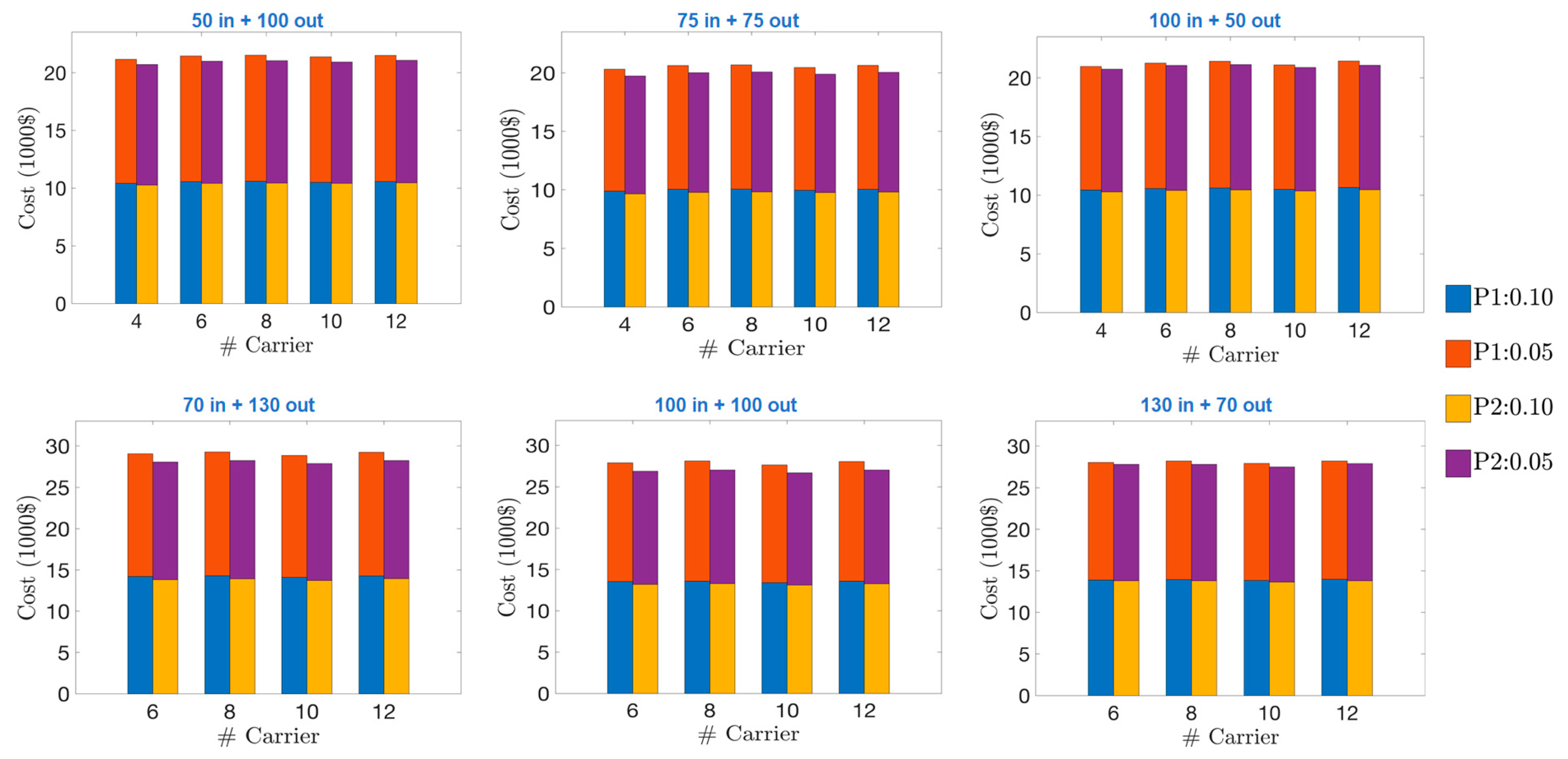
For the stochastic models, the large-scale experiments from Table 5 were performed again using relevant input parameters. Specifically, shipment sizes 50, 100, 150 and 200 were used in the models. In Model 1, only the means and standard deviations of , and are known. For α, β, γ and δ, two different values were used: 0.05 and 0.1. In Model 2, in addition to the means and standard deviations of , and , it is also assumed that the variables follow symmetric probability distributions. Note that the stochastic models do not require explicit assumption about the probability distributions of the travel time variables. This means that there is no need to solve the problems for different replications. Figure 5 presents the results of the experiments for 50 and 100 shipments, and Figure 6 presents the results for 150 and 200 shipments. For example, the subfigure titled “20 in + 30 out” presents the carrier cost of 20 inbound and 30 outbound shipments for 2, 4, 6 and 8 carriers under Propositions 1 and 2. The results of all these experiments show that the carrier cost increases when the user-specified confidence level is increased (i.e., when α, β, γ and δ have a lower value). It can be concluded that increasing the confidence level of the schedule being feasible will result in higher carrier cost. Furthermore, the carrier cost under Proposition 2 is lower than that of Proposition 1 for both values of α, β, γ and δ. This finding corroborates Proposition 3. As evident from Proposition 3, for any values of α, β, γ and δ below 0.5, the carrier cost under Proposition 2 is always lower than that of Proposition 1. Moreover, the assumption of a symmetric travel time distribution can lower the operating cost. The implication of this result is that if carriers were to operate at different times of day (and not only during the peak-hour), they can lower their operating cost.
The results of the above experiments indicate that in order to ensure reliable intermodal collaboration decisions, freight carriers need to consider the uncertainty in travel times. In fact, not considering uncertainty in travel times could cause a truck to miss its appointment at the intermodal terminal/yard or time window at the customer location. Consequently, freight carriers would have a lower service level in the long run. The developed stochastic models provide freight carriers with the ability to design a collaboration plan that would accommodate uncertainty at the desired confidence level. For instance, freight carriers could design a collaboration plan that would be feasible 95% of the time. This capability is crucial for freight carriers that wish to guarantee a certain level of service for their customers. In other words, freight carriers could make guarantees to their customers that they will be able to make the delivery on time. However, there is a trade-off in operating cost. When the desired percentage of on-time delivery is higher, the operating cost will also be higher.
6. Conclusions
This paper provided a strategy for collaboration among freight carriers in domestic intermodal transport. The goal of the framework is to fulfil the participating carriers’ collective demand for inbound and outbound shipments while minimizing the total operating cost. The developed collaboration model resulted in a reduced number of empty container movements by optimally combining inbound and outbound shipments. In all, the collaboration model ensured lower cost for the carriers and the average savings (i.e., cost reduction under collaboration) are shared equally among all participating carriers. Additionally, two stochastic models were provided that take into consideration the uncertainty in truck travel times. These models can be used when a probability distribution for travel times are not available. Model 1 requires only knowing the mean and standard deviation of the travel times, while Model 2 requires in addition that the distribution of the travel times be symmetric. The results indicated that (1) the carrier cost increases as the user-specified level of confidence is increased, and (2) the carrier cost decreases under symmetric travel time distribution for high levels of confidence. The developed models can be used by the domestic intermodal freight carriers to generate optimal and reliable collaborative shipment scheduling.
This paper demonstrated the advantages of horizontal collaboration among freight carriers. However, horizontal collaboration could have drawbacks. Fazili et al. [37] found that horizontal collaboration increases the number of container transfers. It is also conceivable that sharing client/customer information could potentially lead to a loss of businesses to competitors. To date, very few studies have investigated the drawbacks of collaboration. Ferrell et al. [38] indicated in their review paper that more research or case studies are needed.
The proposed framework can be improved in two ways; the model can be extended to include additional or different transport modes, and heuristics could be developed to obtain solutions much faster for large-sized problems.
Author Contributions
Conceptualization, M.U. and N.H.; methodology, M.U.; formal analysis, M.U.; writing—original draft preparation, M.U.; writing—review and editing, M.U. and N.H. All authors have read and agreed to the published version of the manuscript.
Funding
This research received no external funding.
Conflicts of Interest
The authors declare no conflict of interest.
References
- Jennings, B.; Holcomb, M.C. Beyond containerization: The broader concept of intermodalism. Transp. J. 1996, 35, 5–13. [Google Scholar]
- Huynh, N.; Uddin, M.; Minh, C.C. Data analytics for intermodal freight transportation applications. In Data Analytics for Intelligent Transportation Systems; Elsevier: Cambridge, MA, USA, 2017; pp. 241–262. [Google Scholar]
- IANA. Data & Statistics. Available online: https://www.intermodal.org/resource-center/data-statistics (accessed on 15 January 2020).
- Caballini, C.; Sacone, S.; Saeednia, M. Cooperation among truck carriers in seaport containerized transportation. Transp. Res. Part E Logist. Transp. Rev. 2016, 93, 38–56. [Google Scholar] [CrossRef]
- Schulte, F.; Lalla-Ruiz, E.; González-Ramírez, R.G.; Voß, S. Reducing port-related empty truck emissions: A mathematical approach for truck appointments with collaboration. Transp. Res. Part E Logist. Transp. Rev. 2017, 105, 195–212. [Google Scholar] [CrossRef]
- Guajardo, M.; Rönnqvist, M. A review on cost allocation methods in collaborative transportation. Int. Trans. Oper. Res. 2016, 23, 371–392. [Google Scholar] [CrossRef]
- Krajewska, M.A.; Kopfer, H.; Laporte, G.; Ropke, S.; Zaccour, G. Horizontal cooperation among freight carriers: Request allocation and profit sharing. J. Oper. Res. Soc. 2008, 59, 1483–1491. [Google Scholar] [CrossRef]
- Chen, L.; Miller-Hooks, E. Resilience: An indicator of recovery capability in intermodal freight transport. Transp. Sci. 2012, 46, 109–123. [Google Scholar] [CrossRef]
- Uddin, M.; Huynh, N. Reliable routing of road-rail intermodal freight under uncertainty. Netw. Spat. Econ. 2019, 19, 929–952. [Google Scholar] [CrossRef]
- Uddin, M.M.; Huynh, N. Routing model for multicommodity freight in an intermodal network under disruptions. Transp. Res. Rec. 2016, 2548, 71–80. [Google Scholar] [CrossRef]
- Simatupang, T.M.; Sridharan, R. The collaborative supply chain. Int. J. Logist. Manag. 2002, 13, 15–30. [Google Scholar] [CrossRef]
- Cruijssen, F.; Cools, M.; Dullaert, W. Horizontal cooperation in logistics: Opportunities and impediments. Transp. Res. Part E Logist. Transp. Rev. 2007, 43, 129–142. [Google Scholar] [CrossRef] [Green Version]
- Gansterer, M.; Hartl, R.F. Collaborative vehicle routing: A survey. Eur. J. Oper. Res. 2018, 268, 1–12. [Google Scholar] [CrossRef] [Green Version]
- Cong, L.; Zhibin, J.; Feng, C.; Xiao, L.; Liming, L.; Zhou, X. Empty container repositioning—A review. In Proceedings of the WCICA 2010: 8th World Congress on Intelligent Control and Automation, Jinan, China, 7–9 July 2010; pp. 3028–3033. [Google Scholar]
- Özener, O.Ö.; Ergun, Ö. Allocating costs in a collaborative transportation procurement network. Transp. Sci. 2008, 42, 146–165. [Google Scholar] [CrossRef] [Green Version]
- Ergun, Ö.; Kuyzu, G.; Savelsbergh, M. Shipper collaboration. Comput. Oper. Res. 2007, 34, 1551–1560. [Google Scholar] [CrossRef]
- Yilmaz, O.; Savasaneril, S. Collaboration among small shippers in a transportation market. Eur. J. Oper. Res. 2012, 218, 408–415. [Google Scholar] [CrossRef]
- Kuyzu, G. Lane covering with partner bounds in collaborative truckload transportation procurement. Comput. Oper. Res. 2017, 77, 32–43. [Google Scholar] [CrossRef]
- Agarwal, R.; Ergun, Ö. Network design and allocation mechanisms for carrier alliances in liner shipping. Oper. Res. 2010, 58, 1726–1742. [Google Scholar] [CrossRef]
- Atasoy, B.; Schulte, F.; Steenkamp, A. Platform-based collaborative routing using dynamic prices as incentives: The case of Quicargo. In Proceedings of the Transportation Research Board Annual Meeting, Washington, DC, USA, 12–16 January 2020. [Google Scholar]
- Chan, F.T.; Zhang, T. The impact of Collaborative Transportation Management on supply chain performance: A simulation approach. Expert Syst. Appl. 2011, 38, 2319–2329. [Google Scholar] [CrossRef]
- Frisk, M.; Göthe-Lundgren, M.; Jörnsten, K.; Rönnqvist, M. Cost allocation in collaborative forest transportation. Eur. J. Oper. Res. 2010, 205, 448–458. [Google Scholar] [CrossRef] [Green Version]
- Dai, B.; Chen, H. A multi-agent and auction-based framework and approach for carrier collaboration. Logist. Res. 2011, 3, 101–120. [Google Scholar] [CrossRef]
- Los, J.; Schulte, F.; Spaan, M.T.J.; Negenborn, R.R. Collaborative vehicle routing when agents have mixed information sharing attitudes. Transp. Res. Procedia 2020, 44, 94–101. [Google Scholar] [CrossRef]
- Quintero-Araujo, C.L.; Gruler, A.; Juan, A.A. Quantifying Potential Benefits of Horizontal Cooperation in Urban Transportation under Uncertainty: A Simheuristic Approach. In Proceedings of the Advances in Artificial Intelligence, Salamanca, Spain, 14–16 September 2016; pp. 280–289. [Google Scholar]
- Sterzik, S.; Kopfer, H.; Yun, W.-Y. Reducing hinterland transportation costs through container sharing. Flex. Serv. Manuf. J. 2015, 27, 382–402. [Google Scholar] [CrossRef]
- Xue, Z.; Zhang, C.; Lin, W.-H.; Miao, L.; Yang, P. A tabu search heuristic for the local container drayage problem under a new operation mode. Transp. Res. Part E Logist. Transp. Rev. 2014, 62, 136–150. [Google Scholar] [CrossRef]
- Islam, S.; Olsen, T.; Ahmed, M.D. Reengineering the seaport container truck hauling process. Bus. Process Manag. J. 2013, 19, 752–782. [Google Scholar] [CrossRef]
- Tawfik, C.; Limbourg, S. Pricing problems in intermodal freight transport: Research overview and prospects. Sustainability 2018, 10, 3341. [Google Scholar] [CrossRef] [Green Version]
- Tawfik, C.; Limbourg, S. A bilevel model for network design and pricing based on a level-of-service assessment. Transp. Sci. 2019, 53, 1609–1626. [Google Scholar] [CrossRef]
- Ben-Tal, A.; El Ghaoui, L.; Nemirovski, A. Robust Optimization; Princeton University Press: Princeton, NJ, USA, 2009; Volume 28. [Google Scholar]
- Ghosh, B.K. Probability inequalities related to Markov’s theorem. Am. Stat. 2002, 56, 186–190. [Google Scholar] [CrossRef]
- Zhang, R.; Yun, W.Y.; Kopfer, H. Heuristic-based truck scheduling for inland container transportation. OR Spectr. 2010, 32, 787–808. [Google Scholar] [CrossRef]
- USDOT. Freight Facts and Figures; USDOT: Washington, DC, USA, 2017.
- Li, R.; Chai, H.; Tang, J. Empirical study of travel time estimation and reliability. Math. Probl. Eng. 2013, 2013. [Google Scholar] [CrossRef] [Green Version]
- Rakha, H.A.; El-Shawarby, I.; Arafeh, M.; Dion, F. Estimating path travel-time reliability. In Proceedings of the 2006 IEEE Intelligent Transportation Systems Conference, Toronto, ON, Canada, 17–20 September 2006; pp. 236–241. [Google Scholar]
- Fazili, M.; Venkatadri, U.; Cyrus, P.; Tajbakhsh, M. Physical Internet, conventional and hybrid logistic systems: A routing optimisation-based comparison using the Eastern Canada road network case study. Int. J. Prod. Res. 2017, 55, 2703–2730. [Google Scholar] [CrossRef]
- Ferrell, W.; Ellis, K.; Kaminsky, P.; Rainwater, C. Horizontal collaboration: Opportunities for improved logistics planning. Int. J. Prod. Res. 2020, 58, 4267–4284. [Google Scholar] [CrossRef]
Figure 1.
Intermodal freight transportation without collaboration.

Figure 2.
Intermodal freight transportation with collaboration.

Figure 3.
Time window framework for both single and combined shipments.

Figure 4.
Cost variation with problem replications.

Figure 5.
Carrier cost of 50 and 100 shipments under Propositions 1 and 2.

Figure 6.
Carrier cost of 150 and 200 shipments under Propositions 1 and 2.


Table 1.
Overview of related articles focused on freight-oriented horizontal collaborations.
| Focus | Reference | Method | Problem | UC | IM | Equal Profit Share | Shipment/Transport Planning | ||
|---|---|---|---|---|---|---|---|---|---|
| Opt | Game | Sim | |||||||
| Shipper | Ergun et al. [16] | √ | LCP | √ | |||||
| Kuyzu [18] | √ | LCP | √ | ||||||
| Özener and Ergun [15] | √ | √ | LCP | √ | |||||
| Yilmaz and Savasaneril [17] | √ | √ | AP | √ | |||||
| Carrier | Agarwal and Ergun [19] | √ | √ | IP | √ | ||||
| Atasoy et al. [20] | √ | VRP | √ | ||||||
| Caballini et al. [4] | √ | IP | √ | √ | |||||
| Chan and Zhang [21] | √ | AP | |||||||
| Dai and Chen [23] | √ | √ | VRP | √ | |||||
| Frisk et al. [22] | √ | MCFP | √ | √ | |||||
| Islam et al. [28] | √ | AP | √ | ||||||
| Krajewska et al. [7] | √ | √ | VRP | √ | √ | ||||
| Los et al. [24] | √ | VRP | √ | ||||||
| Quintero-Araujo et al. [25] | √ | VRP | √ | √ | |||||
| Schulte et al. [5] | √ | TSP | √ | √ | |||||
| Sterzik et al. [26] | √ | VRP | √ | √ | |||||
| Xue et al. [27] | √ | VRP | √ | √ | |||||
| This study | √ | IP | √ | √ | √ | √ | |||
Opt: Optimization, Game: Game Theory, Sim: Simulation. LCP: Lane Covering Problem, AP: Assignment Problem, IP: Integer Programming, TSP: Travelling Salesman Problem, VRP: Vehicle Routing Problem, MCFP: Minimum Cost Flow Problem. UC: Uncertainty Consideration, IM: Intermodal.
Table 2.
Distance and travel time between the nodes.
| Node | Distance | Travel Time | ||||
|---|---|---|---|---|---|---|
| Intermodal Terminal/ Yard | Shipper/ Receiver | Empty Container Depot | Intermodal Terminal/ Yard | Shipper/ Receiver | Empty Container Depot | |
| Intermodal Terminal/ Yard | 0 | 0 | ||||
| Shipper/Receiver | ||||||
| Empty Container Depot | ||||||
Table 3.
Summary of mathematical notations.
| Notation | Explanation |
|---|---|
| Sets | |
| Set of inbound and outbound shipments | |
| Set of all freight carriers | |
| Set of shipments owned by carrier where | |
| Parameters related to shipments | |
| Origin of shipment | |
| Destination of shipment | |
| Distance traveled by truck when performing shipment ; | |
| Packing/unpacking time at shipper/receiver location related to shipment | |
| Time required when performing shipment ; | |
| Starting time of shipment | |
| Finishing time of shipment ; | |
| Deadline for shipment | |
| Parameters related to carriers | |
| Unit cost of freight carrier , expressed in $/mile | |
| ; this parameter is known in advance | |
| Operating cost of carrier without collaboration | |
| Final operating cost of carrier when performing shipments by itself as well as using HST and VST (with collaboration) | |
| Number of trucks available to carrier | |
| Available time for each truck | |
| Sharing factor, | |
| Parameters related to combined shipments | |
| ; is a sufficiently large number | |
| Distance traveled by truck when performing a pair of shipments ; | |
| Time required when performing a pair of shipments ; | |
| Unit penalty cost of delay | |
| Penalty cost for the delay arising when performing a pair of shipments and violating the deadline of shipment | |
| Finishing time of a pair of shipments ; | |
| Parameters related to time windows | |
| Time windows at the terminal/yard, shippers, and receivers where shipment starts | |
| Time windows at the terminal/yard, shippers, and receivers where shipment ends |
Table 4.
Input data for the shipments in the small-scale experiments.
| Shipment ID | d1 | d2 | Origin | Destination | Carrier | Deadline |
|---|---|---|---|---|---|---|
| 1 | 40 | 35 | Y | ED | 1 | 2 p.m. |
| 2 | 45 | 35 | ED | Y | 1 | 2 p.m. |
| 3 | 55 | 35 | Y | ED | 1 | 2 p.m. |
| 4 | 50 | 33 | ED | Y | 1 | 2 p.m. |
| 5 | 42 | 37 | Y | ED | 1 | 2 p.m. |
| 6 | 37 | 46 | ED | Y | 1 | 2 p.m. |
| 7 | 35 | 32 | Y | ED | 1 | 2 p.m. |
| 8 | 33 | 26 | ED | Y | 1 | 2 p.m. |
| 9 | 40 | 30 | Y | ED | 1 | 2 p.m. |
| 10 | 35 | 28 | ED | Y | 1 | 2 p.m. |
| 11 | 40 | 25 | Y | ED | 2 | 2 p.m. |
| 12 | 35 | 35 | ED | Y | 2 | 2 p.m. |
| 13 | 50 | 40 | Y | ED | 2 | 2 p.m. |
| 14 | 55 | 33 | ED | Y | 2 | 3 p.m. |
| 15 | 61 | 37 | Y | ED | 2 | 2 p.m. |
| 16 | 47 | 46 | ED | Y | 2 | 2 p.m. |
| 17 | 55 | 32 | Y | ED | 2 | 2 p.m. |
| 18 | 63 | 26 | ED | Y | 2 | 3 p.m. |
| 19 | 40 | 30 | Y | ED | 2 | 2 p.m. |
| 20 | 60 | 28 | ED | Y | 2 | 2 p.m. |
| 21 | 30 | 25 | Y | ED | 3 | 2 p.m. |
| 22 | 35 | 40 | ED | Y | 3 | 2 p.m. |
| 23 | 40 | 45 | Y | ED | 3 | 2 p.m. |
| 24 | 60 | 35 | ED | Y | 3 | 2 p.m. |
| 25 | 52 | 47 | Y | ED | 3 | 2 p.m. |
| 26 | 47 | 36 | ED | Y | 3 | 2 p.m. |
| 27 | 40 | 22 | Y | ED | 3 | 2 p.m. |
| 28 | 53 | 24 | ED | Y | 3 | 2 p.m. |
| 29 | 30 | 40 | Y | ED | 3 | 2 p.m. |
| 30 | 42 | 45 | ED | Y | 3 | 2 p.m. |
Table 5.
Model outputs for the small-scale experiments.
| Shipment Type & Cost | CM | ||
|---|---|---|---|
| Carrier 1 | Carrier 2 | Carrier 3 | |
| Single | 6 | 11, 16, 19 | 26, 27 |
| Combined | (1, 28) | (5, 12) | (7, 14) |
| (3, 20) | (17, 2) | (13, 18) | |
| (9, 8) | (21, 24) | (25, 10) | |
| (15, 4) | (23, 22) | (29, 30) | |
| Cost with collaboration ($) | 654.50 | 690.00 | 595.65 |
| Cost without collaboration ($) | 823.90 | 838.00 | 748.60 |
| Savings ($) | 169.40 | 148.00 | 152.95 |
| % Savings | 23.4 | 23.2 | 23.6 |
Table 6.
Computation results with varying number of shipments and carriers.
| Problem Size 1 | Variables # | Constraints # | Cost ($) | Savings ($) | % Savings | Time (s) |
|---|---|---|---|---|---|---|
| 10–20–2 | 1800 | 15,727 | 1872.79 | 534.57 | 22.2 | 4.1 |
| 10–20–4 | 3600 | 29,653 | 1919.15 | 435.55 | 18.5 | 16.0 |
| 10–20–6 | 5400 | 43,579 | 1911.49 | 424.37 | 18.2 | 763.8 |
| 15–15–2 | 1800 | 15,727 | 1771.18 | 636.18 | 26.4 | 3.5 |
| 15–15–4 | 3600 | 29,653 | 1809.45 | 545.25 | 23.2 | 125.0 |
| 15–15–6 | 5400 | 43,579 | 1791.40 | 544.45 | 23.2 | 318.1 |
| 20–10–2 | 1800 | 15,727 | 1903.31 | 504.04 | 20.9 | 31.6 |
| 20–10–4 | 3600 | 29,653 | 1941.00 | 413.70 | 17.6 | 65.0 |
| 20–10–6 | 5400 | 43,579 | 1932.42 | 403.68 | 17.3 | 156.8 |
| 20–30–2 | 5000 | 44,207 | 3120.05 | 909.90 | 22.6 | 8.9 |
| 20–30–4 | 10,000 | 83,413 | 3153.20 | 820.20 | 20.6 | 22.2 |
| 20–30–6 | 15,000 | 122,619 | 3166.97 | 819.54 | 20.5 | 58.6 |
| 20–30–8 | 20,000 | 161,825 | 3105.14 | 802.76 | 20.5 | 1009.6 |
| 25–25–2 | 5000 | 44,207 | 3016.79 | 1013.16 | 25.1 | 9.8 |
| 25–25–4 | 10,000 | 83,413 | 3044.78 | 928.62 | 23.4 | 25.7 |
| 25–25–6 | 15,000 | 122,619 | 3063.56 | 922.94 | 23.2 | 71.2 |
| 25–25–8 | 20,000 | 161,825 | 2998.03 | 909.87 | 23.3 | 217.0 |
| 30–20–2 | 5000 | 44,207 | 3121.63 | 908.33 | 22.5 | 11.8 |
| 30–20–4 | 10,000 | 83,413 | 3153.85 | 819.55 | 20.6 | 28.0 |
| 30–20–6 | 15,000 | 122,619 | 3171.37 | 815.13 | 20.4 | 105.3 |
| 30–20–8 | 20,000 | 161,825 | 3105.80 | 802.00 | 20.5 | 498.0 |
| 30–50–4 | 25,600 | 215,053 | 5208.49 | 1263.76 | 19.5 | 72.7 |
| 30–50–6 | 38,400 | 316,179 | 5204.29 | 1248.21 | 19.3 | 174.0 |
| 30–50–8 | 51,200 | 417,305 | 5213.63 | 1270.77 | 19.6 | 698.6 |
| 30–50–10 | 64,000 | 518,431 | 5195.75 | 1237.06 | 19.2 | 7031.0 |
| 40–40–4 | 25,600 | 215,053 | 4974.91 | 1497.34 | 23.1 | 66.7 |
| 40–40–6 | 38,400 | 316,179 | 4963.40 | 1489.11 | 23.0 | 146.6 |
| 40–40–8 | 51,200 | 417,305 | 4971.60 | 1494.80 | 23.1 | 287.8 |
| 40–40–10 | 64,000 | 518,431 | 4953.96 | 1478.84 | 23.0 | 1082.5 |
| 50–30–4 | 25,600 | 215,053 | 5204.65 | 1267.61 | 19.6 | 72 |
| 50–30–6 | 38,400 | 316,179 | 5192.70 | 1259.80 | 19.5 | 138.8 |
| 50–30–8 | 51,200 | 417,305 | 5201.97 | 1264.43 | 19.5 | 692.9 |
| 50–30–10 | 64,000 | 518,431 | 5181.13 | 1251.67 | 19.4 | 5624.8 |
| 40–60–4 | 40,000 | 336,813 | 6564.33 | 1624.08 | 19.8 | 109.1 |
| 40–60–6 | 60,000 | 495,219 | 6569.62 | 1609.74 | 19.7 | 200.8 |
| 40–60–8 | 80,000 | 653,625 | 6577.55 | 1611.71 | 19.7 | 604.3 |
| 40–60–10 | 100,000 | 812,031 | 6492.52 | 1583.03 | 19.6 | 5798.7 |
| 40–60–12 | 120,000 | 970,437 | 6586.13 | 1606.98 | 19.6 | 39,133.1 |
| 50–50–4 | 40,000 | 336,813 | 6326.87 | 1861.54 | 22.7 | 124.7 |
| 50–50–6 | 60,000 | 495,219 | 6328.50 | 1850.85 | 22.6 | 229.1 |
| 50–50–8 | 80,000 | 653,625 | 6338.15 | 1851.10 | 22.6 | 550.6 |
| 50–50–10 | 100,000 | 812,031 | 6255.36 | 1820.19 | 22.5 | 4106.2 |
| 50–50–12 | 120,000 | 970,437 | 6336.42 | 1856.69 | 22.7 | 8388.2 |
| 60–40–4 | 40,000 | 336,813 | 6559.34 | 1629.06 | 19.9 | 119.7 |
| 60–40–6 | 60,000 | 495,219 | 6568.35 | 1611.01 | 19.7 | 222.2 |
| 60–40–8 | 80,000 | 653,625 | 6574.38 | 1614.87 | 19.7 | 695.7 |
| 60–40–10 | 100,000 | 812,031 | 6486.94 | 1588.61 | 19.7 | 7371.4 |
| 60–40–12 | 120,000 | 970,437 | 6582.86 | 1609.94 | 19.6 | 29,051.1 |
| 50–100–4 | 90,000 | 760,213 | 9954.96 | 2182.49 | 18.0 | 287.2 |
| 50–100–6 | 135,000 | 1,117,819 | 10,092.44 | 2194.51 | 17.9 | 425.1 |
| 50–100–8 | 180,000 | 1,475,425 | 10,136.31 | 2190.89 | 17.8 | 996.6 |
| 50–100–10 | 225,000 | 1,833,031 | 10,042.13 | 2146.98 | 17.6 | 8067.0 |
| 50–100–12 | 270,000 | 2,190,637 | 10,132.66 | 2189.79 | 17.8 | 33,092.3 |
| 75–75–4 | 90,000 | 760,213 | 9398.99 | 2886.15 | 23.5 | 341.8 |
| 75–75–6 | 135,000 | 1,117,819 | 9418.87 | 2868.08 | 23.3 | 485.7 |
| 75–75–8 | 180,000 | 1,475,425 | 9457.52 | 2869.68 | 23.3 | 1078.7 |
| 75–75–10 | 225,000 | 1,833,031 | 9352.02 | 2729.09 | 22.6 | 9700.5 |
| 75–75–12 | 270,000 | 2,190,637 | 9456.35 | 2866.11 | 23.3 | 13,450.2 |
| 100–50–4 | 90,000 | 760,213 | 10,091.23 | 2193.92 | 17.9 | 334.3 |
| 100–50–6 | 135,000 | 1,117,819 | 10,105.71 | 2181.24 | 17.8 | 446.5 |
| 100–50–8 | 180,000 | 1,475,425 | 10,159.74 | 2167.46 | 17.6 | 1022.0 |
| 100–50–10 | 225,000 | 1,833,031 | 10,043.48 | 2145.62 | 17.6 | 8096.7 |
| 100–50–12 | 270,000 | 2,190,637 | 10,153.28 | 2169.17 | 17.6 | 45,806.4 |
| 70–130–6 | 240,000 | 1,990,419 | 13,465.66 | 3123.39 | 18.8 | 1052.6 |
| 70–130–8 | 320,000 | 2,627,225 | 13,561.14 | 3111.52 | 18.7 | 1164.6 |
| 70–130–10 | 400,000 | 3,264,031 | 13,380.36 | 3059.89 | 18.6 | 12,405.4 |
| 70–130–12 | 480,000 | 3,900,837 | 13,567.21 | 3098.04 | 18.5 | 23,480.4 |
| 100–100–6 | 240,000 | 1,990,419 | 12,695.04 | 3894.01 | 23.4 | 1095.8 |
| 100–100–8 | 320,000 | 2,627,225 | 12,773.86 | 3898.80 | 23.4 | 1214.9 |
| 100–100–10 | 400,000 | 3,264,031 | 12,614.22 | 3835.03 | 23.3 | 21,798.7 |
| 100–100–12 | 480,000 | 3,900,837 | 12,791.33 | 3873.93 | 23.2 | 28,036.5 |
| 130–70–6 | 240,000 | 1,990,419 | 13,533.84 | 3055.21 | 18.4 | 1204.5 |
| 130–70–8 | 320,000 | 2,627,225 | 13,638.23 | 3034.42 | 18.2 | 1292.7 |
| 130–70–10 | 400,000 | 3,264,031 | 13,453.29 | 2983.97 | 18.2 | 18,121.4 |
| 130–70–12 | 480,000 | 3,900,837 | 13,648.33 | 3016.92 | 18.1 | 30,413.1 |
1 Number of inbound shipments–number of outbound shipments–number of carriers, # represents number.
© 2020 by the authors. Licensee MDPI, Basel, Switzerland. This article is an open access article distributed under the terms and conditions of the Creative Commons Attribution (CC BY) license (http://creativecommons.org/licenses/by/4.0/).
Share and Cite
MDPI and ACS Style
Uddin, M.; Huynh, N. Model for Collaboration among Carriers to Reduce Empty Container Truck Trips. Information 2020, 11, 377. https://0-doi-org.brum.beds.ac.uk/10.3390/info11080377
AMA Style
Uddin M, Huynh N. Model for Collaboration among Carriers to Reduce Empty Container Truck Trips. Information. 2020; 11(8):377. https://0-doi-org.brum.beds.ac.uk/10.3390/info11080377
Chicago/Turabian StyleUddin, Majbah, and Nathan Huynh. 2020. "Model for Collaboration among Carriers to Reduce Empty Container Truck Trips" Information 11, no. 8: 377. https://0-doi-org.brum.beds.ac.uk/10.3390/info11080377
Note that from the first issue of 2016, this journal uses article numbers instead of page numbers. See further details here.