Article

Quantitative Cluster Headache Analysis for Neurological Diagnosis Support Using Statistical Classification

by
Mohammed El-Yaagoubi
1,2,*,
Inmaculada Mora-Jiménez
1,
Younes Jabrane
2,
Sergio Muñoz-Romero
1,3,
José Luis Rojo-Álvarez
1,3 and
Juan Antonio Pareja-Grande
4
1
Department of Signal Theory and Communications, Telematics and Computing Systems, Rey Juan Carlos University, 28943 Fuenlabrada, Spain
2
MSC Lab, ENSA, Cadi Ayyad University, Marrakech 40000, Morocco
3
Center for Computational Simulation, Universidad Politécnica de Madrid, 28040 Madrid, Spain
4
Department of Neurology, Hospital Universitario Fundación de Alcorcón, 28922 Alcorcón, Spain
*
Author to whom correspondence should be addressed.
Submission received: 1 July 2020 / Revised: 30 July 2020 / Accepted: 6 August 2020 / Published: 10 August 2020
(This article belongs to the Special Issue Signal Processing and Machine Learning)

Abstract

:
Cluster headache (CH) belongs to the group III of The International Classification of Headaches. It is characterized by attacks of severe pain in the ocular/periocular area accompanied by cranial autonomic signs, including parasympathetic activation and sympathetic hypofunction on the symptomatic side. Iris pigmentation occurs in the neonatal period and depends on the sympathetic tone in each eye. We hypothesized that the presence of visible or subtle color iris changes in both eyes could be used as a quantitative biomarker for screening and early detection of CH. This work scrutinizes the scope of an automatic diagnosis-support system for early detection of CH, by using as indicator the error rate provided by a statistical classifier designed to identify the eye (left vs. right) from iris pixels in color images. Systematic tests were performed on a database with images of 11 subjects (four with CH, four with other ophthalmic diseases affecting the iris pigmentation, and three control subjects). Several aspects were addressed to design the classifier, including: (a) the most convenient color space for the statistical classifier; (b) whether the use of features associated to several color spaces is convenient; (c) the robustness of the classifier to iris spatial subregions; (d) the contribution of the pixels neighborhood. Our results showed that a reduced value for the error rate (lower than 0.25) can be used as CH marker, whereas structural regions of the iris image need to be taken into account. The iris color feature analysis using statistical classification is a potentially useful technique to investigate disorders affecting the autonomous nervous system in CH.

1. Introduction

The iris is the eye area located between the pupil and the ciliary region. It contains a variety of grooves, ridges, and pigmented areas, which form a ring bounding the central pupil, through which the light penetrates. The light entering the eye is adjusted by the iris sphincter and dilator. The iris coloration is a physical phenomenon arising from the interaction between the light and the iris stroma. This coloration is due to the melanin concentration, the secretion of which is controlled by the sympathetic nervous system [1].
The iris coloration or the presence of abnormal iris textures has been related to some diseases since remote history, about 1000 years BC. In recent years, diagnostic techniques, evaluation procedures, and treatments have been developed from iris color and texture analysis [2]. Trigeminal autonomic cephalalgias (TACs) belong to Group III of The International Headache Society (IHS), and they share the clinical features of pain felt in the area supplied by the first division (V-1) of the trigeminal nerve, accompanied by a variable combination of cranial autonomic features [1,2]. Cluster headache (CH) is the most frequent TAC [3], and is a male-predominant disorder with a usual age at onset in the late twenties. CH is typically accompanied by very severe strictly unilateral, orbital/periorbital pain, with a variable combination of autonomic features, such as conjunctival injection, lacrimation, rhinorrhea, nasal stuffiness, ptosis, miosis, eyelid edema, and facial/forehead sweating. The attacks last 15–180 min and recur with a frequency from one every other day to 8 per day during symptomatic periods (cluster periods). During attacks of CH, a sympathetic hypofunction is manifested clinically as ptosis and miosis on the painful side. The sympathetic hypofunction remains latent (subclinical) in between attacks, throughout the symptomatic period, but can be unveiled by provocative test with appropriate eye drops substances. If there is a persistent but subtle and constitutional (since birth) sympathetic hypofunction in the symptomatic side, the iris of the symptomatic side would have been less pigmented. In these cases, the sympathetic defect would be congenital or would have occurred in the neonatal period [4,5]. One of the CH signs could be different iris coloration in the patient’s eyes, which is not always noticeable by simple visual inspection. Accordingly, the screening and early detection of CH could be addressed by creating a biomarker from subtle color changes in both eyes’ irises.
Regarding the clinical usefulness of machine learning approaches, many works have been proposed in the literature to deal with different kinds of medical signals and images. As detailed in [6], migraine patients, cluster headache patients, and controls are discriminated using a supervised machine learning approach based on multimodal MRI Study. In [7], a decision support system is proposed to diagnose primary headache patients using semantically enriched data. To support the diagnosis, five primary headache classes were classified using machine learning [8], and a primary headache diagnosis classification task was solved using advanced machine learning techniques [9].
In this paper, we analyze the statistical differences in iris color to develop an automatic quantitative CH diagnosis method by a machine learning approach, in particular the support vector classifier (SVC). We hypothesized that subtle differences in the iris color of both eyes in the same individual could be quantified in terms of the error probability when classifying left and right iris from the pixels of digital iris images. Thus, for each individual, a classification system was designed to determine if a pixel (characterized by color features) belongs to the left/right iris. For this purpose, we considered iris images of both of a patient’s eyes, with images taken under the same conditions. A database of images, specifically recorded for this study, was collected by ophthalmologists in the Hospital Universitario Fundación de Alcorcón in Spain. First, we studied the applicability of statistical classifiers to detect differences in the iris color under a pixel-by-pixel approach. Then, we analyzed the robustness of the classifier to regional changes due to substructures possibly present in the iris images, as well as the impact of simultaneously using features from several color spaces and the contribution of the pixel neighborhood to the classifier performance. A preliminary version of this work was presented in [10].
The paper is outlined as follows. In the next section, we present our image database with patients and control subjects. In Section 3, the classifier approach is introduced. The conducted experiments and results are described, yielding the proposed scheme to generate the CH biomarker from the classification of iris pixels in Section 4. Finally, Section 5 contains conclusions and future perspectives.

2. Image Database

Heterochromia of the eye can sometimes be recognized by the naked eye. Thus, in the example shown in Figure 1, the blue eye is abnormal in terms of noticeably different iris color, which is also confirmed by other signs such as a smaller pupil and subtle drooping of the upper eyelid. In other cases, when the difference is subtle, visual identification can be severely limited. In these cases, an automatic method can be extremely useful for supporting medical diagnosis, which is in line with the approach proposed in this work.
Iris images analyzed in this work were collected by the Ophthalmology Service in Hospital Universitario Fundación de Alcorcón (HUFA) (Madrid, Spain). Original true color images (in RGB format) were acquired under controlled conditions regarding illumination, magnification, and exposition parameters. They were recorded with high resolution (camera Zeiss FF 450 plus Fundus IR, providing images of 768 × 576 pixels) and stored with a digital image file system (451 Visupac Digital, version 3.2.1). To avoid the potential influence of external elements, pictures were centered in the iris by using a circle-shaped frame overlapping the camera. Since the flash effect on the iris cannot always be completely removed, the flash was focused on the pupil center when taking the image. The presence of eyelashes was also minimized at this acquisition stage.
No primary information regarding the symptomatic side of the patient was known by the ophthalmologist who obtained the images. Clinical diagnoses were made by one of the authors (J.A.P-G), and they were in accordance with the diagnostic criteria of the ICH disorders [11]. The database patients was created, with two iris images for each patient (left and right eye). Three subject subsets were considered, namely, subjects with symptomatic CH (Group 1), control subjects (Group 2), and subjects with ophthalmic diseases affecting iris pigmentation (Group 3).

3. Support Vector Classifier Approach

In this work, we propose a statistical-learning approach to support the diagnosis of CH from iris color differences in patients’ eyes. We propose the use of a support vector classifier (SVC) because of its model robustness and good generalization capabilities, arising from the structural risk minimization principle. The SVC principles were developed by Vapnik for the first time [12], and this classifier has since been applied to a dramatically large number of tasks [13].
The design of statistical classifiers such as SVC is conducted by a set of N training samples { x ̲ i , y i } i = 1 N where x ̲ i is the input multivariate sample (also named the input feature vector) and y i is a categorical variable indicating the corresponding label (desired output of the model). From a conceptual point of view, the simplest classifier only has to distinguish between two classes, then coding y i with binary labels +1 and −1. The aim of the SVC is to find the optimal decision boundary based on the maximum margin from the boundary to the training samples of each class. Note that the boundary is just a line in two-dimensional space, which readily extrapolates to a hyperplane in high-dimensional spaces. The decision function can be shown [12] to be expressed as
f ( x ̲ ) = i = 1 L α i y i x ̲ i , x ̲ + b
where . , . denotes the inner product, L is the number of training samples contributing to building the decision boundary, α i are the Lagrange multipliers obtained during the optimization process, and b is the interception or bias term. Samples with a non-zero Lagrange multiplier are known as support vectors.
When samples are not linearly separable in the original input space, Equation (1) does not provide good performance, and input feature vectors are instead nonlinearly mapped to an intermediate high-dimensional feature space. In this case, the SVC constructs an optimal hyperplane in the intermediate space, corresponding to a nonlinear decision boundary in the input space. The expression for the decision function can be shown [12] to be as follows:
f ( x ̲ ) = i = 1 L α i y i K ( x ̲ i , x ̲ ) + b
where K ( . , . ) is a Mercer kernel holding the nonlinear mapping. In our work, the radial basis function (RBF) kernel was used, due to its good performance in many other problems. The RBF kernel, which corresponds to a spherical Gaussian function, has the following expression:
K ( x ̲ , x ̲ i ) = exp | | x ̲ x ̲ i | | 2 2 σ 2
where σ refers to the Gaussian width, for which best value has to be found. When samples of two classes are not fully separable in the transformed space, the SVC includes a penalty term of the structural risk, which is weighted by the hyperparameter C in the optimization process. For large C values, the optimization will choose a lower-margin hyperplane if it achieves a good classification in training. Conversely, a very small value of C will cause the optimization to look for a separation hyperplane with a higher margin, even if the hyperplane misclassifies more training samples [12].

4. Experiments and Results

Several experiments were performed in order to determine the most appropriate color space and the classifier parameters providing the best system operation. On the one hand, the number of pixels required for training was initially scrutinized for SVC. On the other hand, the suitability of different color spaces was analyzed, in particular RGB, Lab, and HSV [14]. In addition, the impact of the possible presence of image structures was tackled by analyzing iris sectors of 45 and creating classifiers to distinguish between the right and left iris using features from different color spaces. Finally, we analyzed the effect of considering as input features the pixel neighborhood, and therefore information about local variability.
To get the iris samples (pixels), the iris was previously segmented from the whole image. This segmentation could not be done automatically with the usual Daugman algorithm [15], since the flash sometimes caused it to fail. Therefore, since the iris segmentation is not the main goal of this paper, it was manually performed using two size-adjustable ellipses for each iris, one for the sclera outer edge and another one for the pupil contour. Figure 2 shows the segmented iris for the left and right eyes in a subject from our database. Pixels outside the area of the segmented iris were discarded in the following stages. To avoid manual intervention, in the future we propose to explore novel graph-based approaches such as FastGCN + ARSRGemb for the iris detection and segmentation [16].
Since the property being scrutinized for use as a CH biomarker is conceptually simple (color differences between pixels from both irises), one might consider using simple statistics on the color image, but we found that it is not so straightforward. Figure 3a shows the histogram of the segmented irises for the red component (RGB space) in a control case (no CH). Example histograms for a patient with CH are given in Figure 3b. Note that the histogram shape for both irises is similar for the control case, as are their means and standard deviations. However, some differences may be observed in the CH example, both in the histogram shape and in their corresponding basic statistics. Nevertheless, simple statistics may not be sufficient for providing a good-quality biomarker. Figure 4 depicts the scatter plot of the iris pixels when using the three components of the color space (Lab and RGB color space in these examples), showing that complex joint distributions can be more informative. In addition, the joint distribution can change with the subject and with the color space. These observations represent the rationale for proposing a classification strategy from machine learning techniques.

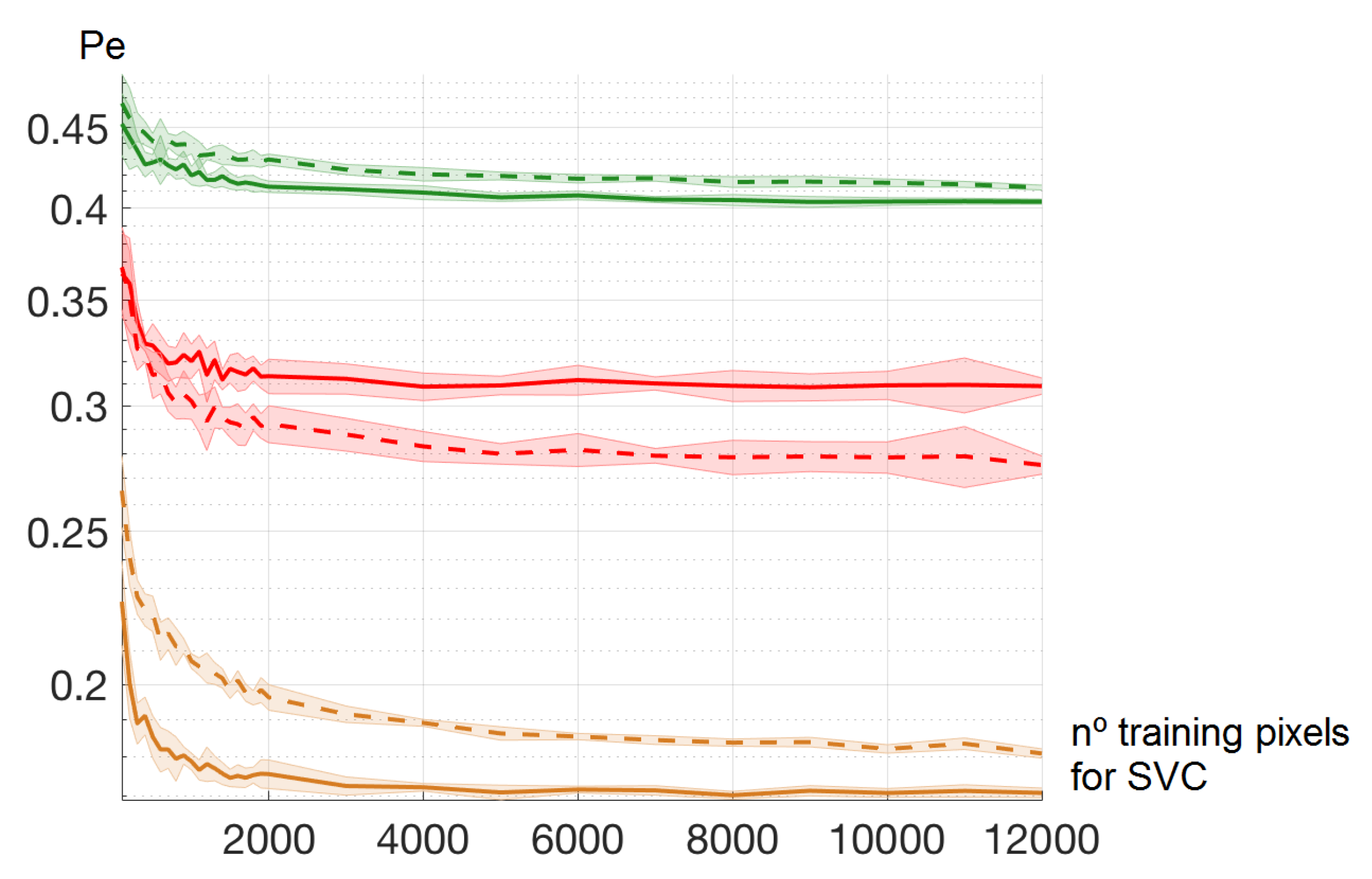
4.1. Number of Training Pixels for SVC Learning

The proposed method for quantifying the presence of differences in pigmentation between both eyes uses the components of the color space as features to characterize pixels. Thus, each pixel corresponds to a sample: the color components are the input features for the classifier, and the label is the identification of the right/left iris that the pixel comes from. For every patient, iris pixels are randomly separated into two subsets, so-called training and test subsets. The training subset is used to build the SVC, and the test subset is used to provide an estimation of the classification error probability, denoted as P e . Note that this separation between training and test subsets makes it possible to check the generalization capabilities of the SVC by using the test pixels, which are different from those used to set the function defining de SVC boundary. In addition, since the RBF kernel implicitly uses the Euclidean distance as a similarity measure between vectors, each input feature is standardized (zero mean and unit variance) to have a similar range.
Hence, the P e estimation provided by a SVC on the iris pixels of both eyes can be used as a simple biomarker for a given patient. It can support the clinician in determining the CH risk of a patient based on color differences between both eyes: the lower the P e , the higher the CH risk. In patients with other pathologies in which differences in eye color are well-known, this method is not necessarily useful. Rather, the usefulness for clinical diagnosis would be focused on CH cases which remain asymptomatic but still exhibit subtle differences in color.
Since the number of available pixels on the iris images was extremely high, it was unnecessary to use all of them for training the classifier. The use of too many training samples would lead to an excessive computational burden in training. Therefore, we first conducted an analysis of how many training samples were needed to yield suitably trained classifiers.
It was also considered convenient to benchmark the SVC with another statistical classifier, in order to confirm that SVC is suitable to tackle this problem. For its conceptual simplicity and performance properties, we chose to use the well-known voting k nearest neighbors (k-NN) classifier, where k is a hyperparameter to be determined [17]. In k-NN, a sample is classified by voting of the labels associated to its k nearest neighbors in terms of the Euclidean distance [18].
Accordingly, the following experiment was conducted to analyze the training set size and the performance of both classifiers (k-NN and SVC). After the iris segmentation of each patient, the same number of pixels ( n p ) were randomly selected for the training and test sets, also balancing the number of pixels for each iris. Pixels in the training set were not considered for selection in the test set. The best values for the hyperparameters of each classifier were selected by cross-validation [19] on the training set. In particular, for the SVC we explored values in the range 1 , 10 5 for the hyperparameter C, and in the range 10 12 , 10 3 for the hyperparameter γ , with γ = 1 2 σ 2 . Regarding the k-NN classifier, the search range for k was 1 , 20 . To avoid the bias provided in the results by one training/test partition, we ran 10 realizations (partitions of the training/test sets) from the complete set of iris pixels. Figure 5 shows the results in terms of P e for two subjects, one being a control and the other a CH patient. Note that for both classifiers, a higher P e was obtained for the control subject. Note that the P e was not 0.5, as this would correspond to a perfectly matched color distribution in both eyes; instead, its value tended to be close to 0.4. The P e value obtained with the CH patient in this case was noticeably lower. Additionally, the P e was generally lower for SVC than for k-NN, which was more pronounced in the CH patient. This result gives the rationale for choosing the SVC as the classifier for building the CH biomarker. Finally, note that at about n p = 2000 , the SVC performance reached stability, hence this was considered a sufficient size for the training set in subsequent experiments.

4.2. Color Spaces

Different color spaces are usually considered in color image processing depending on the scene characteristics and the ultimate goal. Thus, while the RGB color space is considered because its three components (red, green, and blue) are necessary to define the color, other spaces are considered because they consider two components for describing the chromatic information and one component for the achromatic part [14,20].
This section scrutinizes the suitability of different color spaces in our system. In addition to the original RGB color space, we benchmarked its normalized version R G n , where the effect of normalization is a reduced dependence between the red and green components on the brightness, where it possible to omit the third component, hence reducing the space dimensionality [21]. Other color spaces based on linear and nonlinear transformations of their components have been proposed [14,22]. We also considered the Fleck color space [22], based on logarithmic transformations of the RGB components and one of the so-called opponent color spaces. The Fleck transformation is physiologically motivated by the way that the human visual system transforms RGB values into an opponent color vector with one achromatic and two chromatic components. The Otha color components were also considered [23]. They are obtained as a linear transformation of the RGB space, proposed when trying to derive three orthogonal color features with large discriminant power on a representative sample of images. The family of perception-based models are quite intuitive to humans because they are related to human color perception (color, saturation, and luminance): for example, HSI (hue–saturation–intensity) and HSV (hue–saturation–value), which are cylindrical color spaces based on a nonlinear transformation of the RGB space [14]. Finally, the CIE Lab (L for lightness, a and b for color) space was also considered because, in addition to separate chromatic and achromatic components, distance relations (Euclidean) are in accordance with perceptual color differences. The separability of pixels belonging to the left and right iris was benchmarked for each patient when considering the six previously presented color spaces (RGB, HSI, HSV, Otha, Fleck, and Lab) as input features.
The estimated mean error probability on the test set for each patient is shown in Table 1 for the k-NN classifier, and in Table 2 for the SVC. In general terms, the error rate for the SVC was lower than for k-NN. Regarding the input features, and though there were no features which worked best for all patients, we can state that: (1) the color spaces Lab, RGB-Lab, and HSI provided reasonable results when considering the three components of the color space; (2) a b components were the best when just considering chromatic components; and (3) HV and Lb could be selected when choosing the achromatic component and one of the chromatic components, though there were some contradictory trends for some patients. Taking these conclusions into account and analyzing the values of P e , we conclude that input features containing the a b components would be the most appropriate for our purpose. This is in accordance with the similarity measure implicitly considered by the statistical classifiers of this work, since both are based on the Euclidean distance. Nevertheless, other options should not be discarded, such as HSI or RGB-Lab.

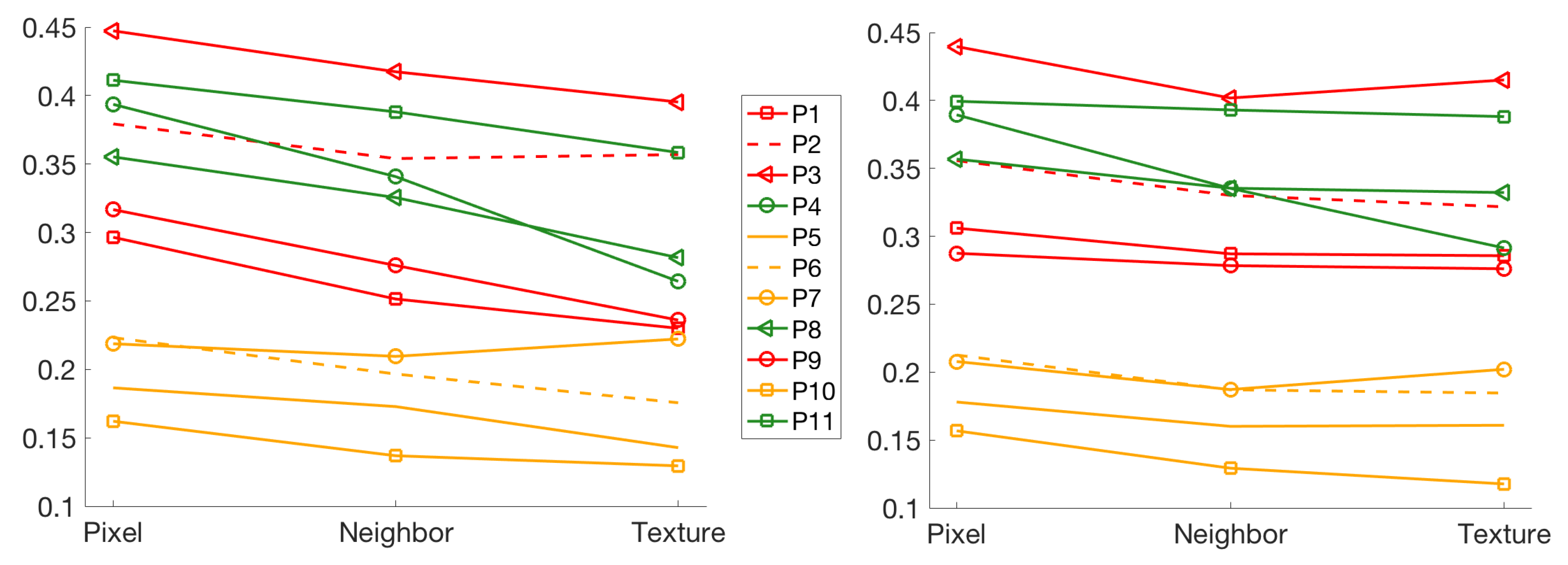
4.3. Effect of Neighbor Pixels and Textures

In the previous experiments, the usefulness of different color components as input features to the classifier was scrutinized on a pixel basis. Despite the color being a pixel property, it is reasonable to analyze whether the color of a given pixel could be better represented by the color of its neighboring pixels. For this purpose, a new feature space was generated by increasing the size of the 3 × 1 vector given by the three components of the pixel in any color space with those provided by the three components associated to its 8 neighboring pixels. Thus, the new feature space is represented by a vector of 27 elements. On the other hand, to get a better characterization of the iris texture, we increased the neighboring size to a distance of 2 pixels. That is, each pixel can be characterized by a vector of 75 elements (25 values per neighborhood and color component).
Figure 6 shows the comparison of input spaces as given by individual pixels and when extending to eight neighbors, and more neighbors (texture). Classifiers were trained and tested with 5000 and 10,000 samples, respectively. Results are shown for the Lab input space. The k-NN classifier showed a defined trend of bringing all the cases closer in terms of P e with increasing pixel neighborhood size, whereas the SVC was less sensitive to the increase of the pixel neighborhood. Nevertheless, there was a trend in some specific cases (specially for patient P4 in the figure) for which P e decreased despite being a control case. Thus, it can be concluded for this problem that feature spaces just associated with individual pixels are better suited than extended spaces considering neighborhood pixels.

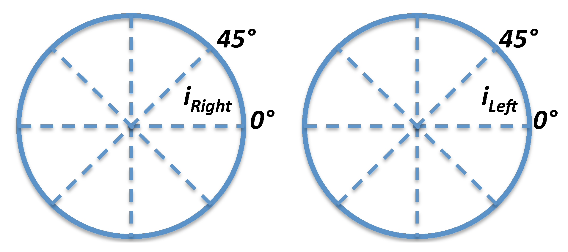
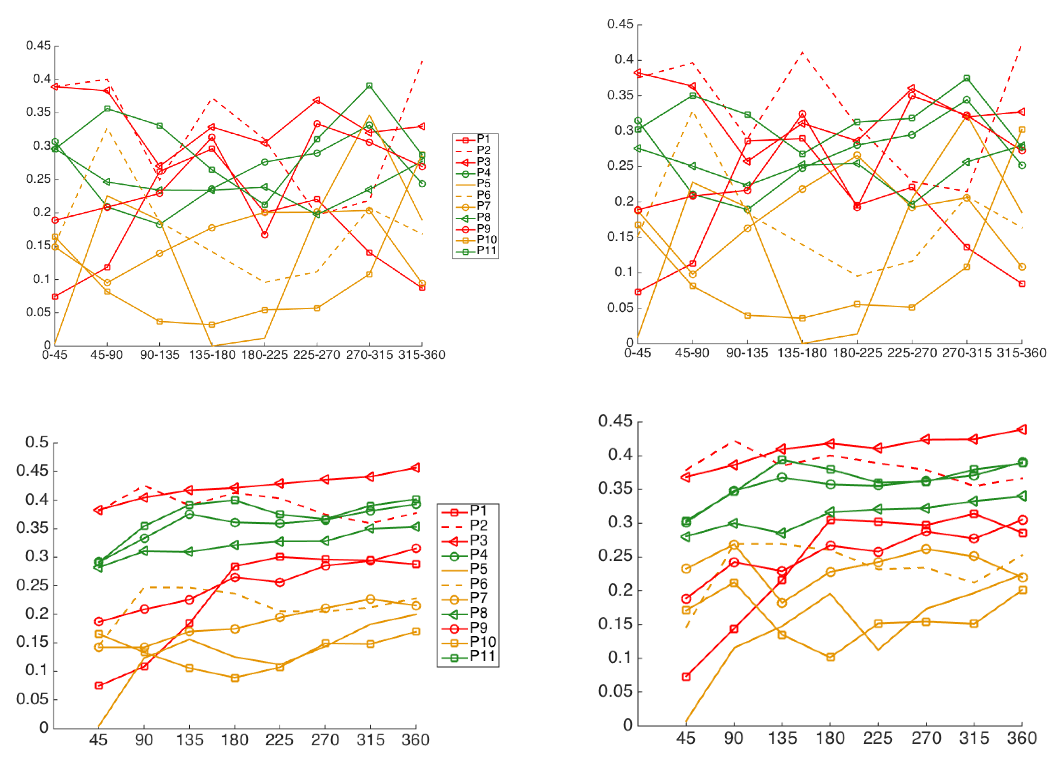
4.4. Iris Image-Region Analysis

In previous experiments, we considered the whole iris area and different numbers of neighbors and components of the color space as features to design the statistical classifier. In addition, some structures can be expected to be present in iris images (e.g., spots or patches), which could modify the color structure and affect the performance of the SVC in this setting. We conducted an experiment for the analysis of the iris by taking the pixels in 45 sectors, as depicted in Figure 7. The features used for this purpose were components of the previously analyzed RGB-Lab space.
We analyzed two strategies. First, a classifier was designed using only those pixels of the same angular sector of the iris in each eye. This approach aimed to account for the presence of structures and for regional differences, which are more noticeable in some sectors than in others. Secondly, the impact of including pixels from increasingly accumulated sectors was also studied. Each classifier was trained with 5000 samples and tested with 10,000 samples for obtaining the P e .
Figure 8 shows that the four patients in Group 3 (P5, P6, P7, and P10) generally exhibited a noticeably reduced P e , which was consistent throughout all angles, although for some sectors their P e was increased. In general terms, the concatenation of all sectors softened the P e and made it constantly low. Additionally, the three healthy subjects in Group 2 showed a consistently increased P e , both in every sector (with some occasional drop in P e ) and in the accumulated figure.
However, results on CH patients in Group 1 exhibited a more complex behavior. In the accumulated classifiers, patients P1 and P9 were readily and consistently identified by the classifiers, P2 showed a trend to be identified but still remained in the P e values of control subjects, and P3 could not be identified and generally exhibited a high P e . On the other hand, the identification by accounting for each sector separately exhibited a larger variance; nevertheless, some sectors were more adequate to better separate Groups 1 and 3 from 2, namely, sectors of 180–225 and 270–315 . Overall, a perfect discrimination could not be achieved. Iris images of patients P2 and P3 often showed a behavior strongly overlapping with an increased P e , which does not seem to support the hypothesis that the iris color features can provide a universal criterion for CH detection, at least as considered in this work. By visual iris inspection on our database, we believe this could mainly be due to two facts: first, the iris tissue in those cases actually contained a variety of spots and marks; and second, the subtle differences in color in these cases were more pronounced in some sectors. Therefore, even when the sector analysis increases the sensitivity, the reduction in the number of pixels makes it more sensitive to spots and marks.

5. Discussion and Conclusions

An SVC-based approach was developed with the aim of supporting the diagnosis of CH with an automatic system. Statistical analysis of its performance was based on sample-based algorithms for learning to classify the pixels of each iris image of the same individual. The corresponding error probability when classifying iris image pixels of an individual was inversely associated to the risk that the individual suffers from CH.
We obtained better CH identification results with features containing both luminance and chrominance information. Additionally, the SVC was a good option as machine learning classifier for use in this task. Moreover, some color spaces were found to be more suitable (Lab, RGB, and HSI). Finally, single-pixel input spaces were found to be better than pixel-neighborhood input spaces. However, CH patients with extremely subtle changes in their eye color could not always be identified by the method. Though this could be alleviated by considering more reduced regions of the iris for increasing sensitivity to color differences, this also increases the sensitivity of the method to marks and spots.
The implications of this study could be clinically relevant. According to recent works, newborns have an inherited and indeterminate iris coloration, which is formed during the first months of life by the cell-coating activity (melanophores). The sympathetic nervous system exerts a trophic action on the activity of the melanophores. When there is a congenital or acquired sympathetic defect in the neonatal period, pigmentation deficiency occurs in the side of the sympathetic hypofunction [4,5]. This results in heterochromia, which can be noted in the different colored eyes, typically blue and brown, with the clearer iris being the defectively pigmented one. Some headaches (typically CH) occur with strictly unilateral pain, centered in the ocular region. During symptomatic periods, a sympathetic deficit on the side of the pain causes ptosis, and miosis is developed. Both signs of sympathetic hypofunction are known as Horner’s syndrome. If there is a latent defect in the sympathetic side of pain that occurs during the symptomatic periods, then there can also be decreased pigmentation of the iris in that side. In that case, sometimes the sympathetic defect has occurred in the neonatal period, and it can sometimes be congenital [5,24].
The present work aimed to open the way towards an automatic diagnostic system. As such, it highlighted the scope and limitations of the color as a sole criterion. The method provided encouraging results, and it arises as a possibility to provide clinicians with diagnostic support for the early detection and screening of CH patients with a low-cost system.

Author Contributions

M.E.-Y. conducted the experiments, organized and wrote the paper, and performed the analysis of experimental results. Y.J., I.M.-J., and J.L.R.-Á. contributed to writing and reviewing the manuscript. S.M.-R. supported the data processing in Matlab. J.A.P.-G. is the neurologist who established the clinical hypothesis and contributed to the database collection and clinical diagnosis. All authors have read and agreed to the published version of the manuscript.

Funding

This work was partially supported by Research Grants BEYOND, KLINILYCS, FINALE, PRINCIPIAS, MAPAS, and KERMES (PID2019-106623RB-C41, TEC2016-75361-R, TEC2016-75161-C2-1-R, TEC2013-48439-C4-1-R, TIN2017-90567-REDT, and TEC2016-81900-REDT) from the Spanish Government.

Conflicts of Interest

The authors declare no conflict of interest.

References

  1. Wielgus, A.; Sarna, T. Melanin in human irides of different color and age of donors. Pigment Cell Res. 2005, 18, 454–464. [Google Scholar] [CrossRef]
  2. McGowan, A.; Silvestri, G.; Moore, E.; Silvestri, V.; Patterson, C.C.; Maxwell, A.P.; McKay, G.J. Retinal Vascular Caliber, Iris Color, and Age-Related Macular Degeneration in the Irish Nun Eye Study. Investig. Ophthalmol. Vis. Sci. 2015, 56, 382–387. [Google Scholar] [CrossRef] [Green Version]
  3. Zebenholzer, K.; Wöber, C.; Vigl, M.; Wessely, P.; Wöber-Bingöl, C. Facial pain in a neurological tertiary care centre–evaluation of the International Classification of Headache Disorders. Cephalalgia 2005, 25, 689–699. [Google Scholar] [CrossRef]
  4. Gladstone, R.M. Development and significance of heterochromia iridis. Arch. Neurol. 1969, 21, 184–192. [Google Scholar] [CrossRef]
  5. Pareja, J.A.; Espejo, M.; Trigo, M.; Sjaastad, O. Congenital Horners Syndrome and Ipsilateral Headache. Funct. Neurol. 1997, 12, 123–131. [Google Scholar] [PubMed]
  6. Messina, R.; Leech, R.; Zelaya, F.; Dipasquale, O.; Wei, D.; Filippi, M.; Goadsby, P. Migraine and Cluster Headache Classification Using a Supervised Machine Learning Approach: A Multimodal MRI Study (P4.10-016). Neurology 2019, 92, 4–10. [Google Scholar]
  7. Vandewiele, G.; De Backere, F.; Lannoye, K.; Vanden Berghe, M.; Janssens, O.; Van Hoecke, S.; Keereman, V.; Paemeleire, K.; Ongenae, F.; De Turck, F. A decision support system to follow up and diagnose primary headache patients using semantically enriched data. BMC Med. Inform. Decis. Mak. 2018, 18, 98. [Google Scholar] [CrossRef] [PubMed]
  8. Keight, R.; Aljaaf, A.J.; Al-Jumeily, D.; Hussain, A.J.; Özge, A.; Mallucci, C. An Intelligent Systems Approach to Primary Headache Diagnosis. In Lecture Notes in Computer Science, Proceedings of the ICIC 2017, Intelligent Computing Theories and Application, Liverpool, UK, 7–10 August 2017; Huang, D.S., Jo, K.H., Figueroa-García, J., Eds.; Springer: Cham, Swizterland, 2017; Volume 10362. [Google Scholar]
  9. Krawczyk, B.; Simic, D.; Simic, S.; Woźniak, M. Automatic diagnosis of primary headaches by machine learning methods. Cent. Eur. J. Med. 2012, 8, 157–165. [Google Scholar] [CrossRef]
  10. El-Yaagoubi, M.; Mora-Jiménez, I.; Rojo-Álvarez, J.L.; Jabrane, Y.; Pareja-Grande, J.A. Extended Iris Color Features Analysis and Cluster Headache Diagnosis Based On Support Vector Classifier. In Proceedings of the IEEE International Conference on Intelligent Systems and Computer Vision (ISCV), Fez, Morocco, 17–19 April 2017. [Google Scholar]
  11. International Headache Society. The international classification of headache disorders. 2nd ed. Cephalalgia 2004, 24, 1–160. [Google Scholar]
  12. Vapnik, V. The Nature of Statistical Learning Theory; Springer: Berlin/Heidelberg, Germany, 2000. [Google Scholar]
  13. Boser, E.; Guyon, I.; Vapnik, V. A training algorithm for optimal margin classifiers. In Proceedings of the Fifth Annual Workshop on Computational Learning Theory, Pittsburgh, PA, USA, 27–29 July 1992; pp. 144–152. [Google Scholar]
  14. Gonzalez, R.C.; Woods, R.E. Digital Image Processing, 4th ed.; Pearson: Harlow, UK, 2018. [Google Scholar]
  15. Daugman, J. The importance of being random: Statistical principles of iris recognition. Patt. Recog. 2003, 36, 279–291. [Google Scholar] [CrossRef] [Green Version]
  16. Manzo, M.; Pellino, S. FastGCN+ARSRGemb: A novel framework for object recognition. arXiv 2020, arXiv:2002.08629. [Google Scholar]
  17. Ghosh, A.K. On optimum choice of k in nearest neighbor classification. Comput. Stat. 2006, 50, 3113–3123. [Google Scholar] [CrossRef]
  18. Cover, T.M.; Hart, P.E. Nearest neighbor pattern classification. IEEE Trans. Inform. Theory. 1968, 13, 21–27. [Google Scholar] [CrossRef]
  19. Trippa, L.; Waldron, L.; Huttenhower, C.; Parmigiani, G. Bayesian nonparametric cross-study validation of prediction methods. Ann. Appl. Stat. 2015, 9, 402–428. [Google Scholar] [CrossRef]
  20. Plataniotis, K.N.; Venetsanopoulos, A.N. Color Image Processing and Applications; Springer: Berlin/Heidelberg, Germany, 2000. [Google Scholar]
  21. Vezhnevets, V.; Sazonov, V.; Andreeva, A. A Survey on Pixel-Based Skin Color Detection Techniques. Proc. Graphicon. 2003, 3, 85–92. [Google Scholar]
  22. Palus, H. Representations of colour images in different colour spaces. In The Colour Image Processing Handbook; Sangwine, S.J., Horne, R.E.N., Eds.; Springer: Boston, MA, USA, 1998; pp. 67–90. [Google Scholar]
  23. Ohta, Y.I.; Kanade, T.; Sakai, T. Color information for region segmentation. Comput. Graph. Image Process. 1980, 13, 222–241. [Google Scholar] [CrossRef]
  24. Krasnianski, M.; Georgiadis, D.; Grehl, H.; Lindner, A. Correlation of clinical and magnetic resonance imaging findings in patients with brainstem infarction. Fortschr. Neurol. Psychiatr. 2001, 69, 236–241. [Google Scholar] [CrossRef] [PubMed]
Figure 1. Screenshots of eyes in a patient with pigmentation deficit when heterochromia is visible to the naked eye.
Information 11 00393 g001
Figure 2. Example of the original right and left iris images (top panels) and their corresponding segmentation (bottom panels).
Information 11 00393 g002
Figure 3. Histograms of the intensity level for the R component (RGB color space) of the segmented iris images (mean ± std) for two patients: (a) a patient with no cluster headache (CH), right iris (95.2 ± 13.4), left iris (93.5 ± 16.0); and (b) a patient with CH, right iris (98.1 ± 13.6); left iris (111.7 ± 20.8).
Information 11 00393 g003
Figure 4. Pixel scatter plot in the Lab space (left panels) and in the RGB space (right panels) for a patient with CH (top panels) and without CH (bottom panels). Red/blue points are respectively associated to the right/left iris pixels.
Information 11 00393 g004
Figure 5. Study of the required number of training pixels for the machine learning classification, benchmarked on a control subject (green), on a different pathology (orange), and on a CH patient (red), when using support vector classifier (SVC; continuous) and k nearest neighbors (k-NN; dashed) classifiers. Shaded bands depict the mean ± standard deviation of 10 realizations.
Information 11 00393 g005
Figure 6. Comparison of the mean P e obtained when considering three approaches (one pixel-based and two extensions to the neighbor pixels, see the abscissa axis), both for k-NN (left panel) and SVC (right panel) classifiers.
Information 11 00393 g006
Figure 7. Scheme of the iris segmentation in 45 sectors for evaluating the impact of image structure on the classifier performance.
Information 11 00393 g007
Figure 8. Study of the P e per iris sector (abscissa axis), for each separate sector (top) and for accumulated sectors (bottom), using k-NN (left panels) and SVC (right panels).
Information 11 00393 g008
Table 1. Mean P e on the test partitions when applying the k-NN classifier on the iris pixels of each patient (rows, organized according to the group to which they belong). Double column headers represents two designs, each one with a different feature space (values in cells keep the order in the column header).
GroupPat. no.RGBLabLaLbabHSIIHIS HS HSI
HSVVHVS HS HSV RG n FleckOhtaRGBLab
10.340.320.340.350.320.350.340.330.35
0.310.380.340.390.340.540.300.31
20.370.390.400.410.420.400.410.410.42
1 0.390.390.420.430.420.500.390.41
30.430.450.490.480.480.470.480.450.45
0.460.450.480.470.470.510.460.47
90.390.380.410.400.440.410.410.400.44
0.380.410.440.430.450.420.380.41
40.440.400.450.440.410.430.450.420.43
0.390.460.440.430.440.470.420.41
80.370.380.400.430.460.370.390.420.41
2 0.350.420.420.430.400.490.360.38
110.430.430.460.460.460.440.460.470.44
0.450.470.470.460.450.500.440.45
50.190.180.210.240.220.210.200.270.24
0.220.190.290.250.240.530.210.21
60.220.200.410.270.240.200.350.240.26
0.230.410.230.230.230.490.200.21
370.280.310.300.380.310.290.340.390.44
0.290.310.350.440.440.500.290.33
100.170.200.220.220.220.180.230.220.24
0.180.250.260.240.230.520.170.17
Table 2. Mean P e on the test partitions when applying the SVC classifier on the iris pixels of each patient (rows, organized according to the group to which they belong). Double column headers represent two designs, each one with a different feature space (values in cells keep the order in the column header).
GroupPat. no.RGBLabLaLbabHSIIHIS HS HSI
HSVVHVS HS HSV RG n FleckOhtaRGBLab
10.320.290.340.320.370.330.330.360.38
0.300.360.320.340.350.470.290.28
20.380.400.410.420.400.400.410.420.41
1 0.380.390.410.410.410.490.380.38
30.440.460.470.480.460.460.470.460.46
0.450.470.470.470.470.490.440.45
90.370.360.380.380.420.360.400.390.42
0.340.400.390.430.430.510.340.37
40.420.390.430.420.440.400.450.420.42
0.390.440.430.400.400.450.410.37
80.360.370.350.420.430.380.370.410.42
2 0.380.420.420.410.430.500.350.32
110.430.430.440.430.400.450.450.430.42
0.480.430.450.440.430.500.430.41
50.190.180.200.240.220.200.190.260.25
0.190.180.250.270.210.520.200.17
60.220.210.390.250.210.190.340.240.24
0.220.380.200.230.230.480.190.18
370.280.270.270.450.390.290.300.390.46
0.270.290.340.450.430.490.280.27
100.170.160.190.190.220.170.200.190.23
0.170.190.230.230.230.480.160.15

