A Fast Algorithm to Initialize Cluster Centroids in Fuzzy Clustering Applications


1
Division of Biometry & Genetics, Çukurova University, Adana 01330, Turkey
2
Department of Electronics & Electrical Engineering, University of Strathclyde, Glasgow G1 1WQ, UK
*
Author to whom correspondence should be addressed.
Information 2020, 11(9), 446; https://0-doi-org.brum.beds.ac.uk/10.3390/info11090446
Submission received: 7 July 2020
/
Revised: 10 September 2020
/
Accepted: 10 September 2020
/
Published: 15 September 2020
(This article belongs to the Special Issue New Trends in Massive Data Clustering)
Abstract
:The goal of partitioning clustering analysis is to divide a dataset into a predetermined number of homogeneous clusters. The quality of final clusters from a prototype-based partitioning algorithm is highly affected by the initially chosen centroids. In this paper, we propose the InoFrep, a novel data-dependent initialization algorithm for improving computational efficiency and robustness in prototype-based hard and fuzzy clustering. The InoFrep is a single-pass algorithm using the frequency polygon data of the feature with the highest peaks count in a dataset. By using the Fuzzy C-means (FCM) clustering algorithm, we empirically compare the performance of the InoFrep on one synthetic and six real datasets to those of two common initialization methods: Random sampling of data points and K-means++. Our results show that the InoFrep algorithm significantly reduces the number of iterations and the computing time required by the FCM algorithm. Additionally, it can be applied to multidimensional large datasets because of its shorter initialization time and independence from dimensionality due to working with only one feature with the highest number of peaks.
1. Introduction
Cluster analysis is one of the main tools of exploratory data analysis in many fields of research and industrial applications requiring image segmentation, computer vision and pattern analysis. The partitioning-based algorithms (a.k.a non-hierarchical or flat algorithms) are probably the most popular among the existing clustering algorithms. A major part of the partitioning algorithms are based on iterative optimization techniques [1]. An iterative optimization task is started with an initial partition of data and then the partitions are iteratively updated by applying a local search algorithm until a convergence criterion is satisfied. Iterations are made by relocating data points between the clusters until a locally optimal partition is found. Since the number of data points in any dataset is always finite, the number of distinct partitions is also finite. The local minima problem could be defeated by using a globally optimal partitioning method [2]. But such exhaustive search methods are ineffective in practice because they require too much of computation time for the globally optimal result. Therefore, a more practical approach is to apply the iterative algorithms which can be divided into two categories such as prototype-based and distribution-based algorithms. The prototype-based algorithms assume that the characteristics of the instances in a cluster can be represented by using a cluster prototype which is a point in the data space. Such algorithms use c prototypes and assign the n instances into the clusters according to their proximity to the prototypes. The objective is to find the clusters that are compact and well-separated from each other.
Although the prototypes of clusters can be centroids or medoids, the former is generally used in most of the applications. The validity of clustering results is closely related to the accurate choice of initial cluster centroids even though an algorithm itself overcomes the coincident clusters problem and is relatively faster than the others. A partitioning algorithm cannot guarantee the convergence to an optimum result because the performance of partitioning depends upon the chosen initial cluster centroids. Thus, the initialization of a prototype-based clustering algorithm is an important step since different choices of the initial cluster centroids can potentially lead to different local optima or different partitions [3]. To get better results, the clustering algorithm, that is, K-means or Fuzzy C-Means (FCM), is run for several times and in each of these runs the algorithm is started with a different set of initial cluster centroids [4]. But this is a highly time-consuming approach especially for high dimensional data. For this reason, the initialization of the partition-based clustering algorithms is a matter of interest [2]. Consequently, faster algorithms estimating the initial cluster centroids are needed in partitioning cluster analyses. The InoFrep (Initialization on Frequency Polygons) algorithm proposed in this paper is a simple data-dependent initialization algorithm which is based on the frequency polygons of features in datasets. The algorithm assumes that the peaks (or the modes) in frequency polygons are the estimates of central tendency locations or the centers of different dense regions, namely the clusters in an examined dataset. Thus, the peaks in frequency polygons can be used for determining the initial cluster centroids in prototype-based cluster analyses.
2. Materials and Methods
2.1. Fuzzy C-Means Clustering and Fuzzy Validity Indices
In a comprehensive survey [5], it is concluded that the clustering algorithm EM and FCM show excellent performance with respect to the quality of the clustering outputs but suffer from high computational time requirements. Hence, the authors of Reference [4] addressed possible solutions relying on programming which may allow such algorithms to be executed more efficiently for big data. In this study, because of its high performance and popularity in the literature we use the original Fuzzy C-means Clustering (FCM) algorithm [6] as the representative of prototype-based clustering algorithms. As a soft clustering algorithm, the FCM differs from the hard K-means algorithm with the use of weighted squared errors instead of using squared errors only. Let be a dataset to be analyzed and be a set of the centroids of clusters in the dataset in dimensional space (, where n is the number of instances, is the number of features and c is the number of partitions or clusters. For the dataset X, the FCM minimizes the objective function in Equation (1).
In Equation (1), of dimension is the membership degrees matrix for a fuzzy partition of .
The element is the membership value of kth instance to the ith cluster. Thus, the ith column of matrix consists of the membership values of n instances to the ith cluster. is a cluster prototypes matrix defined in Equation (3):
In Equation (1), is the distance between kth data point and the centroid of the ith cluster. It is computed using a squared inner-product distance norm as in Equation (4):
is a positive and symmetric norm matrix in Equation (4). The inner product with is a measure of distances between data points and cluster prototypes. When is equal to , is obtained in squared Euclidean norm. In Equation (1), is a fuzzifier parameter (or weighting exponent) whose value is chosen as a real number greater than 1 . While m approaches to 1, clustering tends to become crisp but when it approaches to the infinity clustering becomes more fuzzified. The value of m is usually set to 2 in most of the applications. The objective function JFCM is minimized with the constraints given in Equations (5)–(7):
The FCM stops when the number of iterations has reached a predefined maximum number of iterations or when the difference between the sums of membership values in , obtains two consecutive iterations that are less than a predefined convergence value (. The steps involved in the FCM are:
- Initialize the membership matrix and the prototype matrix .
- Update the cluster prototypes:
- Update the membership values with:
- If then stop else go to the step 2, where is the iteration number.
For evaluating the effect of initialization algorithms on the clustering results of the FCM, we use the fuzzy clustering validation indices listed in Table 1. The indices of Partition Entropy and Modified Partition Coefficient use partition matrix only, whereas the indices of Xie-Beni, Kwon and PBMF use , and as shown in the formulas in Table 1. Therefore, even if the latter ones require more execution time, it is expected that they may give more accurate validation of partitioning by using the dataset itself and centroids matrix in addition to the fuzzy membership matrix.
2.2. Related Works on Initialization of Cluster Centroids
To generate the initial cluster centroids matrix V, in the first step of prototype-based algorithms, the principal rule is to find the data points that are close enough to the final centers of the clusters and they should be reasonably far from each other for different clusters. In this case, convergence will be quicker to return a good clustering result. For this goal, we could iterate over all the points to determine where the distances are the maximum between them. However, such an iterative approach can be seen as ineffective and already done by the partitioning algorithms themselves. Hence, we need computationally effective methods and many of them are already present in the literature. In a comprehensive review [1], the initialization methods are broadly categorized into three groups as the data-independent, the simple and the sophisticated data-dependent methods. The data-independent methods completely ignore the data points. On the other hand, the simple data-dependent methods use the data points in initialization by random sampling them whereas the sophisticated data-dependent methods use data points in more complicated fashions. Despite their simplicity, the data-independent methods have many disadvantages and hence, not preferred in the clustering applications.
The initialization by random sampling process on datasets (so-called Irand in this paper) is the simplest data-dependent method in which the random samples are drawn from the dataset without replacement for using the prototypes of each cluster. The Irand has been applied in many clustering implementations due to its simplicity and computational efficiency. The grid block method [12] divides the data space into the blocks and searches for the dense regions. A grid block is considered as the indicator of a cluster center if the number of data points in it is greater than a given threshold value. Although this method works well for two-dimensional datasets, it has some disadvantages for multidimensional data and also presents difficulties in selection of the thresholds.
Although there are several sophisticated data-dependent approaches, for example, Particle Swarm Optimization [13], the most interesting representatives of these methods are Mountain clustering [14] and, Subtractive clustering [15]. Mountain clustering [14] is a method for approximate estimation of cluster centers on the basis of density measures. Despite the relative simplicity and effectiveness of this method, its computational cost increases exponentially when the dimensions of the patterns grow since the method must evaluate the mountain function over all grid points [3]. In Subtractive clustering as an alternative one-pass algorithm [15], instead of grids points, the data points are processed as the candidates of cluster centroids in the dataset. By using this method, the computational cost is simply proportional to the number of data points and free from the dimension problem that arises with the Mountain method. Applying these methods is difficult because they require the input parameters which should be configured by the users [3]. The K-means++ [16] is another approximation algorithm overcoming the poor clustering problem, which sometimes happens with the classical K-means algorithm. K-means++ (called ‘kmpp’ in this paper) initializes the cluster centers by selecting the data points that are farther away from each other in a probabilistic manner. The kmpp is a recommended method in the clustering applications because of its several advantages versus the methods above discussed.
The first two methods above discussed are deterministic, giving the same cluster centroids for every run on the same dataset while the kmpp is non-deterministic. In some of the studies the deterministic methods are recommended because of lower computational complexity but some others suggest to use the non-deterministic ones because of their empirically proven effectiveness on the real datasets [17]. For this reason, we have selected the Irand as the representative of simple data-dependent methods and the kmpp as the representative of sophisticated data-dependent methods. As shown in the following sections, the InoFrep is a data-dependent algorithm that uses the peaks on the frequency polygon of the feature with the highest number of peaks. Using the values of these peaks as the initial values of the cluster centers, the algorithm InoFrep enables the clustering algorithms approach to the final clustering results faster. This significantly reduces the number of iterations and the computation time required by the clustering algorithms. Since the cluster initial values are determined with only a single-pass of the algorithm, it also provides the advantage of using the same initial values in the repetitive runs of the clustering algorithms. In the following sections, we introduce the InoFrep and compare its effectiveness with those of the Irand and the kmpp.
2.3. Proposed Algorithm: Initialization on Frequency Polygons
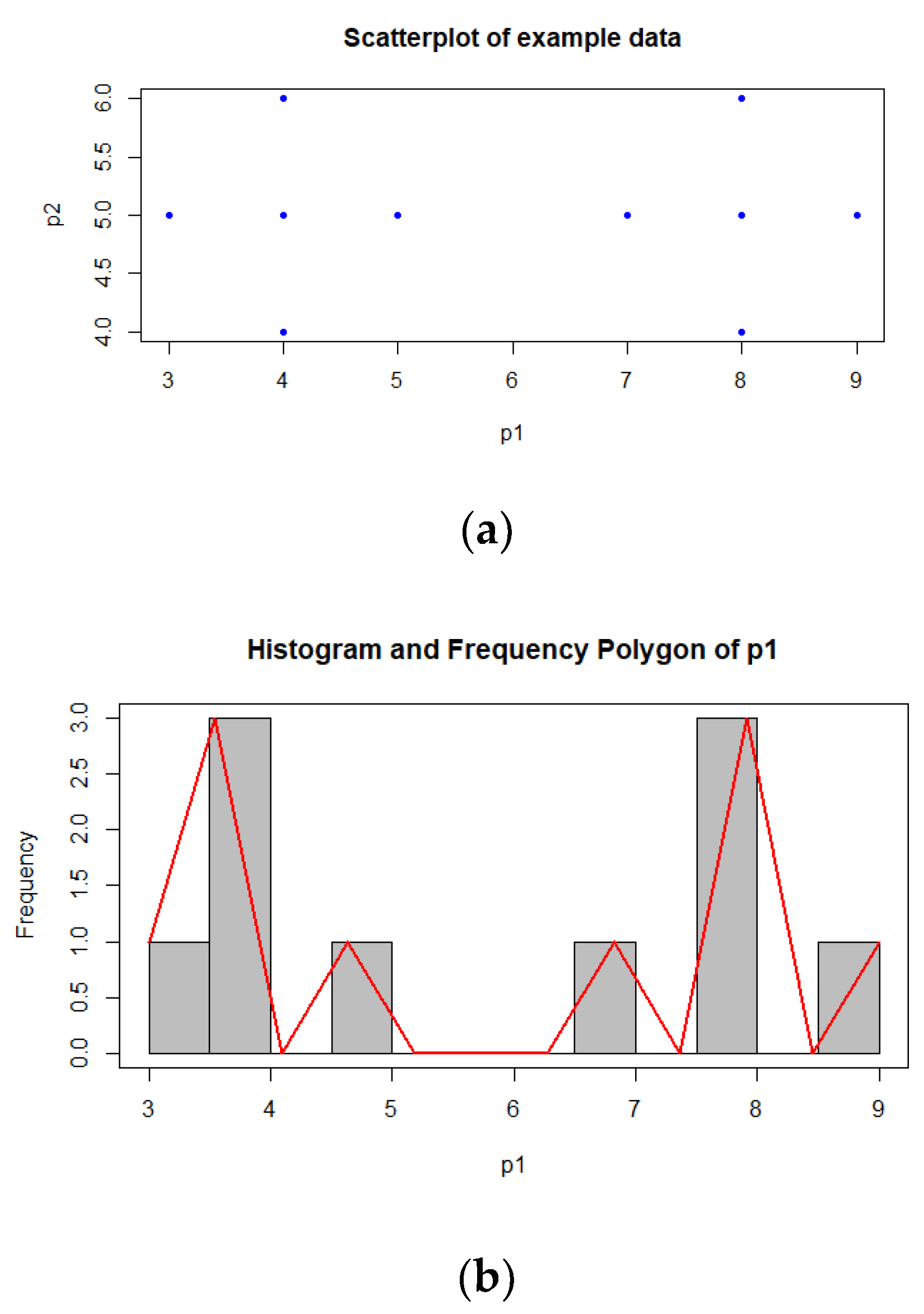
To explain the logic behind the proposed algorithm, a small numerical data of 10 observations of the two features (p1 and p2) is given as following:
p1 = {5, 8, 7, 4, 8, 4, 3, 8, 9, 4}
p2 = {5, 6, 5, 4, 5, 6, 5, 4, 5, 5}
As it is seen from the scatter plot p1 vs p2 in Figure 1a, two well-separated clusters do exist in this two dimensional simple dataset. As demonstrated in the figure, the center points of these two clusters are v1 = (4, 5) and v2 = (8, 5). If the cluster centroids are initialized with the values close to these central points (v1 and v2), clustering algorithms will approach to the actual cluster centers with a few iterations. Thus, starting the clustering algorithms with initial values which are close to the real cluster centers can remarkably reduce the computing time required in clustering analysis. In the descriptive statistics, histograms and frequency polygons are used as visual tools for understanding and comparing the shapes of distributions of features in a dataset [18]. In a frequency polygon, the x-axis represents the values of c classes of features and the y-axis indicates the frequency of each class. Therefore, frequency polygons also serve structural information about the data. The values of peaks of a feature are the modes of data representing the most repeated instances [18], and, thus, they can be used as the prototypes of cluster centers in datasets. The histograms and frequency polygons of the features p1 and p2 in our simple example data are shown in Figure 1b,c, respectively. The values (pv1 and pv2) and frequencies (pc1 and pc2) of these peaks are given below:
- pv1 = {3.75, 4.75, 6.75, 7.75, 8.75}; pc1 = {3, 1, 1, 2, 1}
- pv2 = {4.75, 5.75}; pc2 = {6, 2}
As shown in the frequency polygon mid values above, there are five peaks for the feature p1 and there are two peaks for the feature p2. Since the peaks indicate the presence of subgroups or clusters in the studied data, we can assume that there are 5 clusters according to the first feature and 2 clusters according to the second feature. The value of the peak with the highest frequency can be used as the center coordinates of the first cluster, which in our example is 3.75. Then the value of the peak with the second high frequency will be used as the initial value of the first cluster, which is 7.75 in our example. These initial values are very close to the values of actual center of the first cluster for p1. When the same operations are done for p2, the peak values 4.75 and 5.75 are assigned as the initial values of the first and second clusters. If the number of peaks determined for a feature is less than the number of clusters (parameter c) given as the input argument in the cluster analysis, the other clusters can be initialized with random sampling.
For finding the peaks and obtaining the values of peaks to be used as the initial centroids, we have developed the findpolypeaks algorithm (Algorithm 1). The input arguments of this algorithm are the frequencies and middle values of the classes of frequency polygon of the analyzed feature (xc and xm respectively), a threshold counts value (tc) for filtering purposes. The output returned by the algorithm is a peaks matrix PM. At the beginning of the findpolypeaks, the frequencies and middle values of the frequency polygon are filtered and the frequencies below a threshold value, tc are removed from xc. The default value of tc is 1 that means that all 0’s and 1’s are removed from xc because they are not needed or might be noises (Line 1 in Algorithm 1). In this way, the valleys and possible noises in the frequency vector of frequency polygons are eliminated from xc and xm for making the process faster and more robust. Then, the number of classes in xc is computed (nc) and an index for the peaks (pidx) is started at 1.
| Algorithm 1. findpolypeaks |
| Input: xc, vector for the frequencies of classes (or bins) of a frequency polygon xm, vector for the middle values of classes (or bins) of a frequency polygon tc, threshold frequency value for filtering frequency polygon data, default value is 1 Output: PM: Peaks matrix for a feature Init: 1: xc ← xc [xc >= tc]; xm ← xm [xc >= tc] //Filter xm and xc for the class frequencies >= tc 2: pfreqs ← {} //Atomic vector for the frequencies of peaks 3: pvalues ← {} // Atomic vector for the values of peaks 4: nc ← length of xc //Number of classes (or number of bins) 5: pidx ← 1 //Index of the first peak Run: 6: IF nc > 1 THEN 7: IF xc [1] > xc [2] THEN 8: pvalues [1]← xm [1]; pfreqs [1]← xc [1] 9: pidx ← 2 10: ENDIF 11: FOR i = 2 to nc-1 DO 12: IF xc [i] not equal to xc [i − 1] THEN 13: IF xc [i] > xc [i − 1] AND xc [i] >= xc [i + 1] THEN 14: pvalues [pidx] ← xm [i] 15: pfreqs [pidx] ← xc [i] 16: pidx ← pidx + 1 17: ENDIF 18: ENDIF 19: ENDFOR 20: IF xc [nc] > xc [nc − 1] THEN 21: pvalues [pidx]← xm [nc]; pfreqs [pidx]← xc [nc] 22: ENDIF 23: ELSE 24: pvalues [pidx] ← xm [1]; pfreqs [pidx]← xc [1] 25: ENDIF 26: np ← length of pvalues 27: PMnpx2 ← 0 //Create peaks matrix 28: PM [1] ← pvalues; PM [2] ← pfreqs 29: RETURN PM, np |
If xc contains only one element (one frequency value), it is returned as the peak of the analyzed feature (Line 24 in Algorithm 1). Otherwise, the frequencies in xc are examined to find the peaks of analyzed feature (Lines 6–22 in Algorithm 1). If the first frequency value in xc is greater than the second value, it is assigned as the first peak value; and pidx, which the index for peaks is increased by 1 (Lines 7–10 in Algorithm 1). Then a loop is performed on the remaining frequency values for finding the other peaks (Lines 11–19 in Algorithm 1). If the ith frequency value is greater than previous (i − 1th) and next (i + 1th) frequency values in xc, it is flagged as a peak and the pidx is increased one (14–16 in Algorithm1). One last control is performed whether a last peak does exist or not (Lines 20–22 in Algorithm 1). Finally, the peaks matrix PM consists of np rows and 2 columns is generated and returned by the findpolypeaks. The values and the frequencies of the peaks found by the algorithm are stored in the first and second columns of PM respectively (Line 28 in Algorithm 1).
The InoFrep algorithm (Algorithm 2) uses three input arguments: Xnxp, dataset as a matrix (n: number of instances, p: number of features), c, number of clusters and nc, number of classes for generating frequency polygons. Here, nc is determined heuristically. If a number greater than the actual number of clusters in the dataset has been chosen for the nc, the algorithm will remove the gaps between the bins thus it will not become a major problem for finding the peaks. For instance, in our experiments with the synthetic dataset in the next section where nc is chosen as 20 while the actual number of clusters is 4, the algorithm does not struggle to determine the peaks counts. The output of the algorithm is the initial centroids matrix of c rows and p columns. In the initialization phase of the algorithm, all elements of V matrix are set to 0 and an atomic vector peakcounts is generated to store the frequencies of peaks in the analyzed frequency polygon (Lines 1–2 in Algorithm 2).
The frequency polygon of feature j is generated and the mid values and the frequencies of the classes are stored in two atomic vectors (jmids and jcounts in Algorithm 2 respectively; see Lines 4–5 in Table 2 for the examined dataset). The algorithm findpolypeaks with these input arguments and the number of peak frequencies for the feature j is stored as the jth value of the vector peakcounts (Lines 7–8 in Algorithm 2). Then, the feature index with the highest peak counts is determined as maxj and its frequency polygon is generated (Lines 10–11 in Algorithm 2). Next, findpolypeaks is called with the middle values and the frequencies of the classes of frequency polygon for the feature maxj, the feature with maximum peak counts. The returned peaks matrix PM is ordered on the peak frequencies in descending order and PMS matrix is obtained (Lines 12–18 in Algorithm 2). The peak values in the first column of PMS are used to find the closest points to them in the dataset. The found data point of the feature maxj is assigned as the centroid of the ith cluster (Line 21 in Algorithm 2). If the number of peaks is less than the number of clusters to be used by the clustering algorithm, the centroids of the remaining clusters (c-np clusters) are generated with randomly sampled data points of the feature maxj (Line 25 in Algorithm 2). The randomly sampled points are checked for duplicates to prevent coincided cluster centroids (Lines 26–32 in Algorithm 2). The above-described processes are repeated until the number of clusters and finally the initial centroids matrix V is returned to the clustering algorithm.
| Algorithm 2. InoFrep |
| Input: Xnxp, dataset as matrix (n: number of instances, p: number of features) c, Number of clusters used by the partitioning algorithm nc, Number of classes to generate frequency polygons Output: Vnxc, Initial centroids matrix Init: 1: V [i,j] ← 0 //Set 0 to V matrix; i = 1,…,c; j = 1,...,p 2: peakcounts ← { } //Atomic vector to store the peak counts Run: 3: FOR each feature j DO 4: COMPUTE the middle values and frequencies from the frequency polygon of the feature j using nc 5: jmids ← {Middle values of the classes of frequency polygon of feature j} 6: jcounts ← {Frequencies of the classes of frequency polygon of feature j} 7: CALL findpolypeaks with jmids and jcounts 8: peakcounts [j] ← number of rows of PM //number of peaks for the feature j from findpolypeaks 9: ENDFOR 10: maxj ← index of max{peakcounts} 11: COMPUTE the middle values and frequencies from the frequency polygon of the feature maxj using nc 12: midsmaxj ← {Middle values of the classes of frequency polygon of the feature maxj} 13: countmaxj ← {Frequencies of the classes of frequency polygon of the feature maxj} 14: CALL findpolypeaks with midsmaxj and countmaxj 15: np ← number of peak counts for the feature maxj from the findpolypeaks algorithm 16: PM [1] ← {Peak values of the feature maxj} 17: PM [2] ← {Peak frequencies of the feature maxj} 18: PMS ← SORT PM on the 2nd column in descending order and store in PMS 19: i ← 1 20: WHILE i <= c DO 21: IF i ≤ np THEN 22: //Find the nearest data point of the feature maxj to the ith peak value 23: idx ← argmin{|X [,maxj]–PMS [i,1]|} 24: ELSE 25: REPEAT 26: duplicatedcenters ← false 27: idx ← rand(X [,maxj]) // One random sample on the feature maxj 28: FOR k = 1 to i − 1 29: IF X [idx, maxj] = V [k,maxj] THEN 30: duplicatedcenters ← true 31: ENDIF 32: ENDFOR 33: UNTIL not duplicatedcenters 34: ENDIF 35: FOR each feature j DO 36: V [i,j] ← X [idx, j] 37: ENDFOR 38: INCREMENT i 39: ENDWHILE 40: RETURN V |
3. Results and Discussion
3.1. Experiment on a Synthetic Dataset
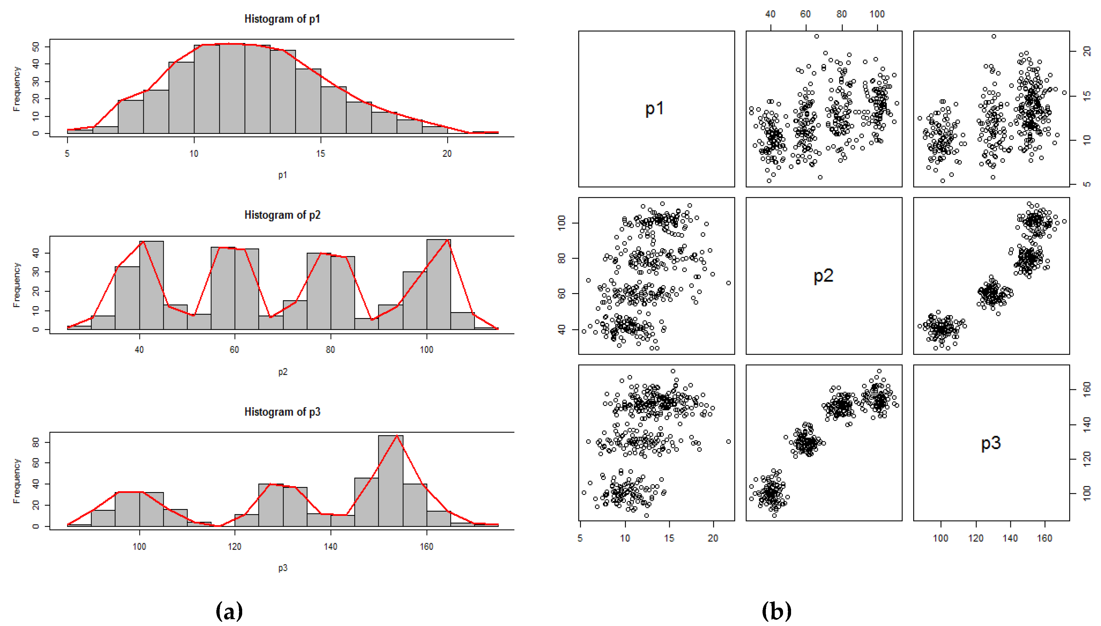
In this study, the findpolypeaks and the InoFrep algorithms have been implemented in R [19] and tested on a computer with i7–6700HQ CPU (2.60 GHz) and 16GB RAM. For comparison of the InoFrep to the others, we have also coded the R functions for the kmpp and the Irand algorithms (See Supplementary Materials). To evaluate the performance of the compared algorithms, we have generated a synthetic dataset (3P_4C) by using the rnorm function of base stats library of R. The dataset consisted of three mixture Gaussian features with the descriptive statistics shown in Table 2. The first feature (p1) is unimodal, the second feature (p2) is four modal and third feature (p3) is three modal as seen in Figure 2a. Although the number of instances in the created example synthetic dataset is arbitrarily chosen as 400 to easily monitor the distribution and scattering of the points in the graphics, working with a smaller and larger number of instances does not affect the relative success of the proposed algorithm because it only uses the modes to initialize the cluster centers.
In our experiment, we run the FCM for six levels of the number of clusters (c = 2,…,7) with each of the three initialization algorithms (InoFrep, kmpp and Irand). In each level of the number of clusters, the FCM is started for ten times because the Irand and the kmpp algorithms determine different centroids in different runs due to the non-deterministic nature of these algorithms. In order to prevent the possible biases due to different membership matrix U initialization, we used the same U matrix for each level of the number of clusters in repeated runs of the FCM.
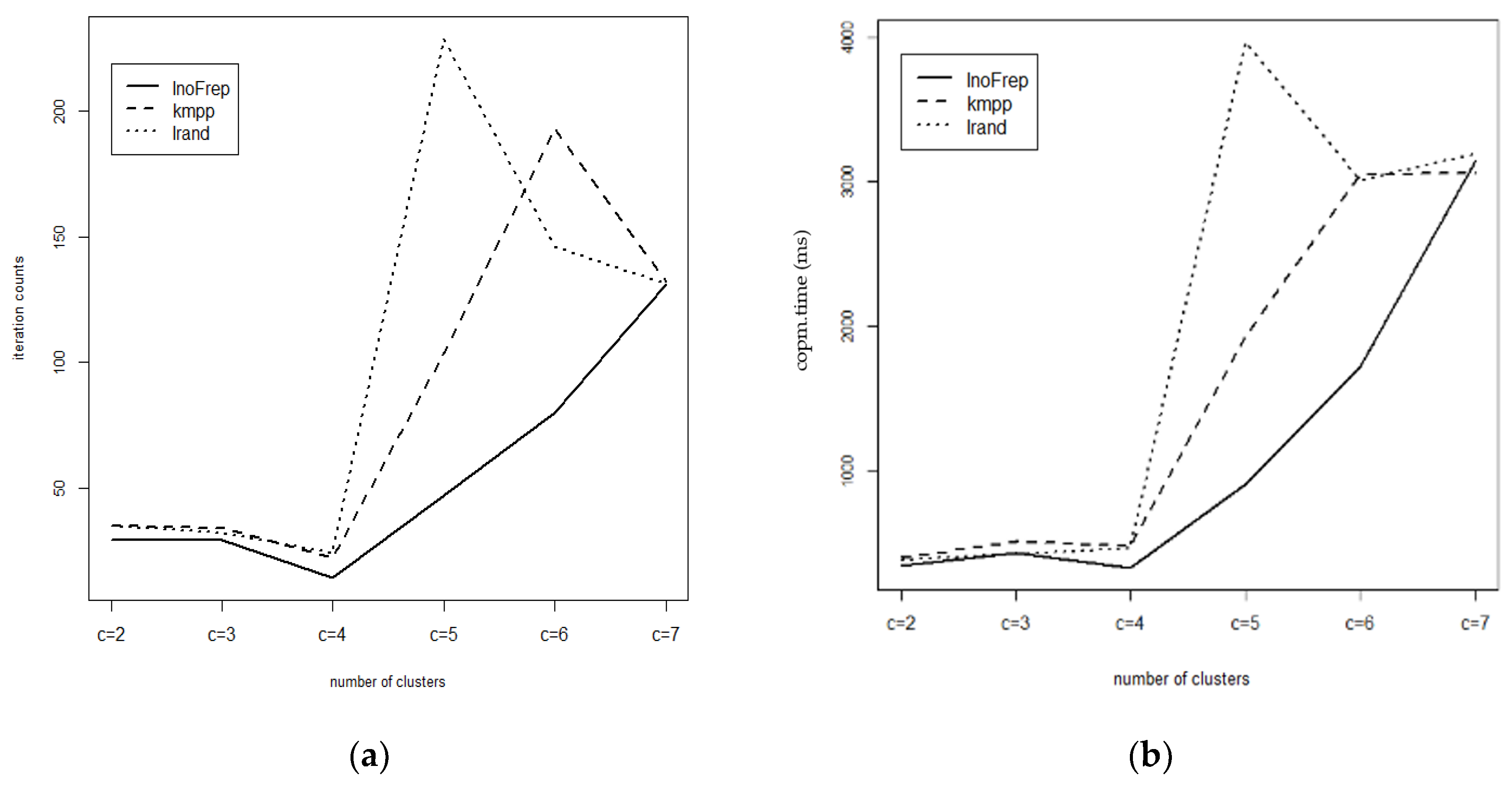
The results obtained from the FCM runs on the 3P_4C dataset are shown in Table 3. In this table, imin, iavg, imax and isum, respectively, stand for the minimum number of iterations, the average number of iterations, the maximum number of iterations and the total number of iterations in ten runs of the FCM. As another performance criterion, ctime in Table 3 shows the total computing time (milliseconds) for ten runs of the FCM. In the last row of Table 3, itime stands for the average computing time of the initialization algorithms for evaluating their initialization performances. As seen in Table 3, the InoFrep requires a smaller number of iterations and computing time when compared to the kmpp and the Irand (the best results are shown in bold in the table). The kmpp is in the middle and the Irand is the worst (Chi-Sq. = 26.503, df = 10, p = 0.00312). As clearly seen from Figure 3a,b, the performances of all of the algorithms converges to each other when c is 7. If the number of clusters processed by the FCM is greater than the maximum peak counts found by the InoFrep, the centroids for the last c-np clusters are generated with random sampling technique (see Line 25 in Algorithm 2). In this case, although the performance of the InoFrep becomes similar to the performances of the kmpp and the Irand although this is a rare occasion for most of the data, however, running the FCM for larger c values will not be reasonable.
In parallel to the number of iterations, the computing times required by the FCM are also significantly different between the compared initialization algorithms (Chi-sq = 279.58, df = 10, p < 2.2 × 10⁻¹⁶). According to the results in Table 3, the InoFrep requires less computing time when compared to those required by the kmpp and the Irand. The InoFrep is especially better than the kmpp and the Irand when the number of clusters approached to the number of actual clusters in the analyzed datasets. Moreover, another superiority of the InoFrep is due to its stability between different runs of the FCM. While the kmpp and the Irand do not ensure the same initialization values from one run to another, the InoFrep presents the same values between runs of clustering algorithms below the number of peaks (np). Because, the InoFrep is considered as a semi-deterministic algorithm and it does not need the repeated runs for testing of a better initialization. In other words, just one run of the InoFrep guarantees the same initialization results if np for the selected feature is less than the number of clusters (c) passed to the FCM. Consequently, the number of iterations required by the FCM with the initial centroids generated by the InoFrep are significantly less than those of the compared algorithms. Thus it indicates that the InoFrep has higher computational efficiency. At the same time, since the algorithm uses the modes of features it takes the present structure of the dataset into account and hence reinforces the noise robustness.
In our study, the fuzzy index values computed from membership matrices returned by all the FCM runs are the same. As seen in Table 4, the indices of XB and Kwon suggests three clusters while PBMF, MPC and PE suggests four clusters. As visible in Figure 2b above, three or four natural groupings might be obtained for 3P_4C synthetic dataset. Therefore, although both of these results are acceptable, we could conclude that PMBF, MPC and PE suggests an accurate number of clusters for the examined dataset.
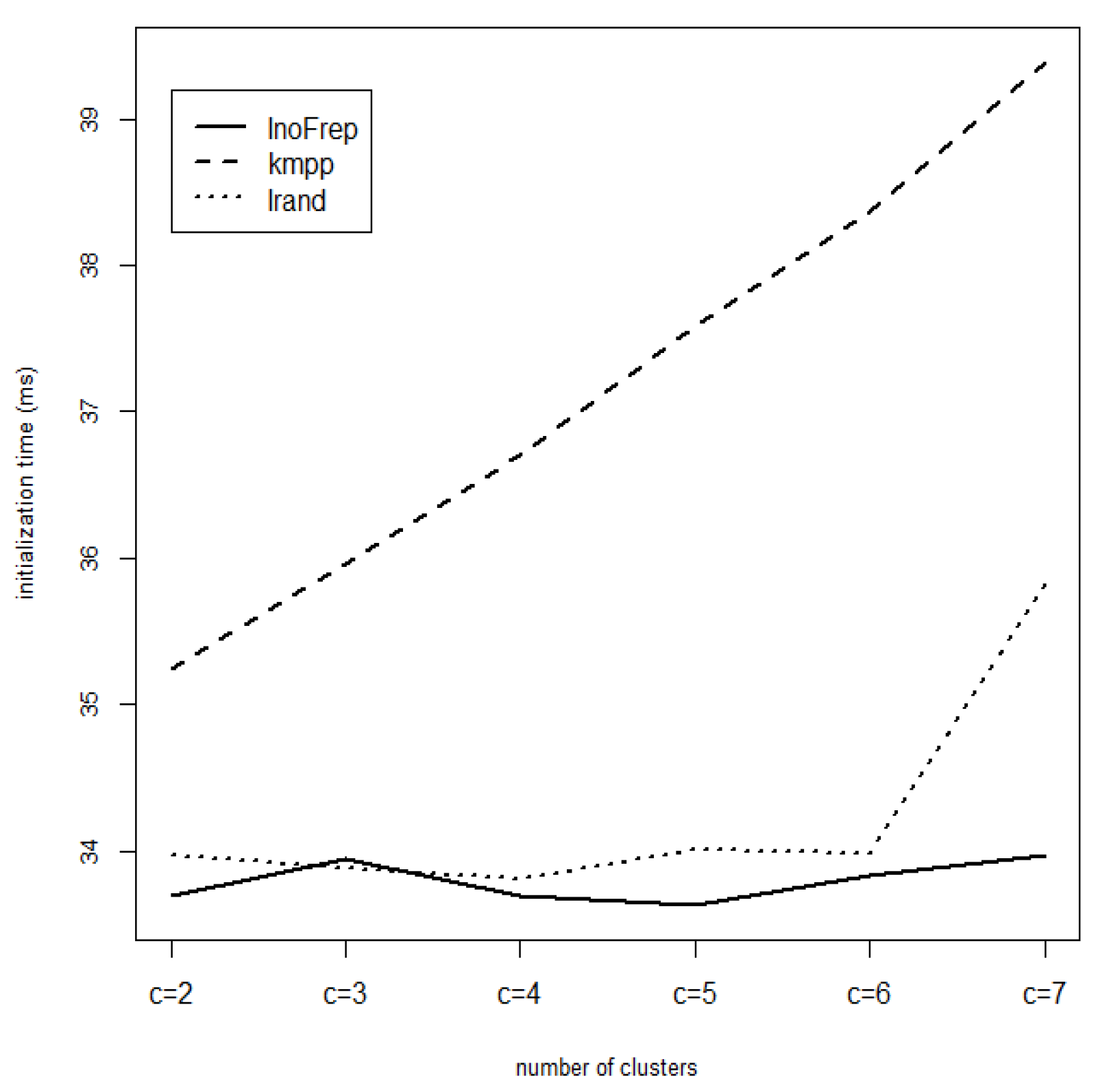
In the literature, performance evaluation of the algorithms focuses mostly on the comparison of the number of iterations and computing time required by the clustering algorithms as done above. In this study, we have also investigated the performances in initialization step itself. As seen in Figure 4 and the last row of Table 3, the time required by three initialization algorithms (itime) differs significantly. The InoFrep required less initialization time at all levels of the number of clusters. The initialization time of the kmpp increases linearly and is longer than those of the Irand and the InoFrep. However, the initialization time required by the InoFrep and the Irand is more or less close to each other, although it is longer for the Irand for the clustering at c = 7.
3.2. Experimental Results on Real Datasets
In order to compare the performances of the tested initialization algorithms we used six real datasets from UCI Machine Learning Repository [20]. The definitions of these datasets are given in Table 5. In this table, p, c, ec and sp respectively stand for the number of features, the number of clusters, the estimated number of clusters by the fuzzy indices in Table 1 and the index of selected feature with large number of peaks in the related datasets.
The results obtained with the InoFrep, the kmpp and the Irand on the real datasets are given in Table 6, Table 7 and Table 8 respectively. In regard of average number of iterations (iters) and computing time (ctime) required by the FCM, the InoFrep performs relatively better than the kmpp and the Irand for most of the real datasets. The InoFrep outperforms in the clustering sessions done with the cluster numbers which are equal and close to the actual cluster numbers in the examined real datasets. The Irand is also good in some clustering sessions for Iris, Forest and Wine datasets especially in the clustering sessions done with large number of clusters. The InoFrep algorithm uses the same technique with the Irand for the clustering done with larger clusters above the actual number of clusters in an examined dataset, its performance becomes similar to the Irand. On the other hand, since the Irand produces different results in different runs, the InoFrep could be preferred due to its deterministic nature and single-pass efficiency for initialization of cluster centroids for high-dimensional datasets in data mining applications.
4. Conclusions
In this paper, we have proposed a new algorithm to initialize cluster centroids for the prototype-based clustering algorithms. The InoFrep finds the data points close to the peaks of frequency polygon of the feature with the highest peak counts and assigns them as the initial centroids. Since the peaks are the modes of central tendency of data points, the selected initial prototypes become close to the actual centers of clusters. Due to this proximity, the number of iterations and computing time required by the clustering algorithms are significantly reduced. Therefore, the InoFrep algorithm may produce better initialization values when compared to the Irand and the kmpp for clustering sessions done with cluster numbers which are equal and close to the actual cluster numbers in examined datasets. Since the kmpp selects the first centroid and minimum probable distance that separates the centroids at random, different results can be obtained in different runs of it. For getting a better result, the kmpp has to be run several times [21]. On the other hand, the InoFrep produces the same results in only one pass of it. The InoFrep also reduces the risk of selection of outliers in the datasets and thereby reinforces more robustness because it always selects the central tendency points.
The InoFrep algorithm is easy to implement and proves to be an alternative method to determine initial centroids which can be used in prototype-based partitioning such as probabilistic and possibilistic fuzzy clustering as well as hard clustering algorithms. Besides providing speed-up the InoFrep is also applicable to high dimensional datasets because of its deterministic nature.
Supplementary Materials
The implementations of the algorithms compared in this study are available online at https://cran.r-project.org/web/packages/inaparc/inaparc.pdf. Package ‘inaparc’- CRAN-R Project.
Author Contributions
Conceptualization, Z.C. and C.C.; methodology, Z.C.; software, Z.C. and C.C.; validation, C.C.; formal analysis, C.C.; resources, Z.C.; data curation, Z.C.; writing—original draft preparation, Z.C. and C.C.; visualization, C.C.; supervision, Z.C. All authors have read and agreed to the published version of the manuscript.
Funding
This research received no external funding.
Conflicts of Interest
The authors declare no conflict of interest.
References
- Borgelt, C. Prototype-based Classification and Clustering; Habilitationsschrift zur Erlangung der Venia Legendi für Informatik, vorgelegt der Fakultaet für Informatik der Otto-von-Guericke-Universitaet Magdeburg: Magdeburg, Germany, 2005. [Google Scholar]
- Äyrämö, S.; Kärkkäinen, L. Introduction to Partitioning-based Clustering Methods with a Robust Example. In Reports of the Department of Mathematical Information Technology (University of Jyväskylä) Series C: Software and Computational Engineering C1; University of Jyväskylä: Jyväskylän, Finland, 2006; pp. 1–36. [Google Scholar]
- Kim, D.-W.; Lee, K.H.; Lee, D. A novel initialization scheme for the fuzzy c-means algorithm for color clustering. Pattern Recognit. Lett. 2004, 25, 227–237. [Google Scholar] [CrossRef]
- Moertini, V.S. Introduction to five clustering algorithms. Integral 2002, 7, 87–96. [Google Scholar]
- Fahad, A.; Alshatri, N.; Tari, Z.; Alamri, A.; Khalil, I.; Zomaya, A.; Foufou, S.; Bouras, A. A survey of clustering algorithms for big data: Taxonomy and empirical analysis. IEEE Trans. Emerg. Top. Comp. 2014, 2, 267–279. [Google Scholar] [CrossRef]
- Bezdek, J.C. Pattern Recognition with Fuzzy Objective Function Algorithms; Plenum Press: New York, NY, USA, 1981. [Google Scholar]
- Bezdek, J.C. Cluster validity with fuzzy sets. J. Cybern. 1973, 3, 58–73. [Google Scholar] [CrossRef]
- Dave, R.N. Validating fuzzy partitions obtained through c-shells clustering. Pattern Recognit. Lett. 1996, 17, 613–623. [Google Scholar] [CrossRef]
- Xie, X.L.; Beni, G. A validity measure for fuzzy clustering. IEEE Trans. Pattern Anal. Mach. Intell. 1991, 13, 841–847. [Google Scholar] [CrossRef]
- Kwon, S.H. Cluster validity index for fuzzy clustering. Electron. Lett. 1998, 3, 2176–2178. [Google Scholar] [CrossRef]
- Pakhira, M.K.; Bandyopadhyay, S.; Maulik, U. Validity index for crisp and fuzzy clusters. Pattern Recognit. 2004, 37, 487–501. [Google Scholar] [CrossRef]
- Zou, K.; Wang, Z.; Hu, M. A new initialization method for fuzzy c-means algorithm. Fuzzy Optim. Decis. Mak. 2008, 7, 409–416. [Google Scholar] [CrossRef]
- Xianfeng, Y.; Pengfei, L. Tailoring fuzzy c-means clustering algorithm for big data using random sampling and particle swarm optimization. Int. J. Database Theory Appl. 2015, 8, 191–202. [Google Scholar] [CrossRef]
- Yager, R.R.; Filev, D.P. Generation of fuzzy rules by mountain clustering. J. Intell. Fuzzy Syst. 1994, 2, 209–219. [Google Scholar] [CrossRef]
- Chiu, S. Fuzzy model identification based on cluster estimation. J. Intell. Fuzzy Syst. 1994, 2, 267–278. [Google Scholar] [CrossRef]
- Arthur, D.; Vassilvitskii, S. K-means++: The Advantages of Careful Seeding. In Proceedings of the 18th Annual ACM-SIAM Symposium on Discrete Algorithms, New Orleans, LA, USA, 7–9 January 2007; Gabow, H., Ed.; Society for Industrial and Applied Mathematics: Philadelphia, PA, USA, 2007; pp. 1027–1035. [Google Scholar]
- Stetco, A.; Zeng, X.-J.; Keane, J. Fuzzy c-means++: Fuzzy c-means with effective seeding initialization. Expert Syst. Appl. 2015, 42, 7541–7548. [Google Scholar] [CrossRef]
- Aitnouri, E.M.; Wang, S.; Ziou, D.; Vaillancourt, J.; Gagnon, L. An Algorithm for Determination of the Number of Modes for Pdf Estimation of Multi-modal Histograms. In Proceedings of the Vision Interface 99, Trois-Rivieres, QC, Canada, 18–21 May 1999; pp. 368–374. [Google Scholar]
- R Core Team. R: A Language and Environment for Statistical Computing; R Foundation for Statistical Computing: Vienna, Austria, 2013; Available online: https://www.R-project.org (accessed on 28 December 2019).
- UCI Machine Learning Repository. Available online: http://archive.ics.uci.edu/ml (accessed on 28 December 2019).
- Pavan, K.K.; Rao, A.P.; Rao, A.V.D.; Sridhar, G.R. Robust seed selection algorithm for k-means type algorithms. Int. J. Comput. Sci. Inf. Technol. 2011, 3, 147–163. [Google Scholar]
Figure 1.
(a) Scatter plot for the features p1 and p2 in the example data (b) Histogram and frequency polygon of the feature p1 (c) Histogram and frequency polygon of the feature p2.
Figure 1.
(a) Scatter plot for the features p1 and p2 in the example data (b) Histogram and frequency polygon of the feature p1 (c) Histogram and frequency polygon of the feature p2.


Figure 2.
(a) Histograms and frequency polygons of the features in 3P_4C dataset (b) Pairwise scatter plots of the features in 3P_4C dataset.
Figure 2.
(a) Histograms and frequency polygons of the features in 3P_4C dataset (b) Pairwise scatter plots of the features in 3P_4C dataset.

Figure 3.
(a) Iteration counts by the number of clusters (b) Computing time (ms) required in the number of clusters.
Figure 3.
(a) Iteration counts by the number of clusters (b) Computing time (ms) required in the number of clusters.

Figure 4.
Initialization time (ms) by the compared initialization algorithms.


Table 1.
Internal validity indices for validation of fuzzy clustering results.
| Index | Index Formula |
|---|---|
| Partition Entropy [7] | |
| Modified Partition Coefficient [8] | |
| Xie-Beni Index [9] | |
| Kwon Index [10] | |
| PBMF Index [11] |
Table 2.
Descriptive statistics and frequency polygon data of the features in 3P_4C dataset.
| Features | p1 | p2 | p3 |
|---|---|---|---|
| Number of instances | 400 | 400 | 400 |
| Mean | 12.29 | 70.02 | 133.94 |
| Standard deviation | 2.86 | 22.69 | 22.02 |
| Frequencies of classes | 2 4 19 25 41 51 52 51 48 37 27 18 12 8 4 0 1 | 2 7 33 46 13 8 43 42 7 15 40 38 6 13 30 47 9 1 | 1 15 32 32 16 4 0 11 40 37 12 10 46 86 40 14 3 1 |
| Mid values of classes | 5.5 6.5 7.5 8.5 9.5 10.5 11.5 12.5 13.5 14.5 15.5 16.5 17.5 18.5 19.5 20.5 21.5 | 27.5 32.5 37.5 42.5 47.5 52.5 57.5 62.5 67.5 72.5 77.5 82.5 87.5 92.5 97.5 102.5 107.5 112.5 | 87.5 92.5 97.5 102.5 107.5 112.5 117.5 122.5 127.5 132.5 137.5 142.5 147.5 152.5 157.5 162.5 167.5 172.5 |
| Number of peaks | 1 | 4 | 3 |
| Values of peaks | 11.5 | 42.5 57.5 77.5 102.5 | 97.5 127.5 152.5 |
| Frequencies of peaks | 52 | 46 43 40 47 | 32 40 86 |
Table 3.
Iteration counts and execution time required by the compared initialization algorithms.
| c = 2 | c = 3 | c = 4 | |||||||
| Kmpp | InoFrep | Irand | Kmpp | InoFrep | Irand | Kmpp | InoFrep | Irand | |
| imin | 34 | 29 | 34 | 29 | 29 | 29 | 17 | 14 | 14 |
| iavg | 35 | 29 | 35 | 34 | 29 | 32 | 22 | 14 | 24 |
| imax | 35 | 29 | 36 | 34 | 29 | 32 | 23 | 14 | 25 |
| isum | 351 | 290 | 352 | 341 | 290 | 319 | 273 | 140 | 245 |
| ctime | 402.05 | 345.06 | 383.43 | 508.24 | 435.01 | 426.15 | 477.79 | 325.88 | 462.42 |
| itime | 35.24 | 33.70 | 33.97 | 35.96 | 33.95 | 33.88 | 36.70 | 33.70 | 33.81 |
| c = 5 | c = 6 | c = 7 | |||||||
| Kmpp | InoFrep | Irand | Kmpp | InoFrep | Irand | Kmpp | InoFrep | Irand | |
| imin | 48 | 47 | 43 | 57 | 80 | 83 | 77 | 80 | 78 |
| iavg | 104 | 47 | 229 | 142 | 80 | 146 | 120 | 131 | 131 |
| imax | 132 | 47 | 250 | 193 | 80 | 150 | 132 | 147 | 136 |
| isum | 1038 | 470 | 2292 | 1423 | 800 | 1457 | 1205 | 1311 | 1660 |
| ctime | 1934.24 | 909.68 | 3970.68 | 3051.58 | 1722.15 | 3007.69 | 3060.21 | 3147.02 | 3194.27 |
| itime | 37.59 | 33.63 | 34.01 | 38.36 | 33.84 | 33.98 | 39.39 | 33.97 | 35.82 |
Table 4.
Index values computed from membership matrix of 3P_4C dataset.
| IXB | IKwon | IPBMF | IMPC | IPE | |
|---|---|---|---|---|---|
| c = 2 | 0.06398359 | 25.84344 | 1.112161 × 10⁴ | 0.6855225 | 0.1996096 |
| c = 3 | 0.05879530 | 24.19019 | 4.466028 × 10⁵ | 0.7490964 | 0.1941429 |
| c = 4 | 0.07750218 | 33.07070 | 7.096132 × 101 | 0.7850980 | 0.1768860 |
| c = 5 | 0.65254444 | 279.28554 | 1.284663 × 10⁶ | 0.6786742 | 0.2800888 |
| c = 6 | 0.70858359 | 306.77753 | 8.637914 × 10⁶ | 0.6237016 | 0.3345075 |
| c = 7 | 0.79080017 | 345.13123 | 7.018537 × 10⁶ | 0.5474565 | 0.4175081 |
Table 5.
The real datasets used to compare the performances of compared algorithms.
| Dataset | n | p | c | ec | sp |
|---|---|---|---|---|---|
| Iris | 150 | 4 | 2–3 | 2 | 2 |
| Forest | 198 | 27 | 4 | 4–5 | 5 |
| Wine | 178 | 13 | 3 | 2 | 8 |
| Glass | 214 | 9 | 6 | 2–3 | 7 |
| Vaweform | 5000 | 21 | 3 | 2–3 | 8 |
| Wilt train | 4889 | 6 | 2 | 2 | 1 |
Table 6.
Performance of the InoFrep algorithm on the real datasets.
| c = 2 | c = 3 | c = 4 | c = 5 | c = 6 | ||||||
|---|---|---|---|---|---|---|---|---|---|---|
| Dataset | iters | ctime | iters | ctime | iters | ctime | iters | ctime | iters | ctime |
| Iris | 16 | 117.81 | 37 | 223.11 | 69 | 442.58 | 55 | 453.90 | 157 | 1368.10 |
| Forest | 46. | 253.65 | 57 | 397.24 | 32 | 317.61 | 105 | 1073.27 | 146 | 1729.45 |
| Wine | 24 | 146.06 | 70 | 407.61 | 57 | 417.63 | 93 | 784.84 | 256 | 2428.10 |
| Glass | 28 | 174.91 | 43 | 315.07 | 55 | 465.42 | 175 | 1661.62 | 94 | 1099.79 |
| Vaweform | 32 | 3164.89 | 50 | 7146.28 | 210 | 38,958.49 | 433 | 107,249.2 | 233 | 67,886.63 |
| Wilt train | 39 | 3133.99 | 94 | 10,993.57 | 116 | 17,744.25 | 316 | 60,230.48 | 258 | 59,319.35 |
Table 7.
Performance of the kmpp algorithm on the real datasets.
| c = 2 | c = 3 | c = 4 | c = 5 | c = 6 | ||||||
|---|---|---|---|---|---|---|---|---|---|---|
| Dataset | iters | ctime | iters | ctime | iters | ctime | iters | ctime | iters | ctime |
| Iris | 17 | 122.07 | 40 | 238.38 | 68 | 455.57 | 78 | 614.10 | 98 | 938.85 |
| Forest | 43 | 250.92 | 63 | 460.88 | 33 | 343.51 | 98 | 1072.61 | 123 | 1589.85 |
| Wine | 26 | 157.96 | 69 | 414.39 | 57 | 442.89 | 199 | 1684.91 | 107 | 1128.61 |
| Glass | 27 | 175.51 | 91 | 609.56 | 59 | 518.89 | 75 | 792.68 | 95 | 1156.62 |
| Vaweform | 33 | 3466.88 | 57 | 8480.23 | 231 | 44,947.23 | 443 | 108,892.3 | 234 | 69,624.66 |
| Wilt train | 43 | 3584.90 | 105 | 12,644.0 | 179 | 28,135.95 | 303 | 59,471.17 | 197 | 46,778.42 |
Table 8.
Performance of the Irand algorithm on the real datasets.
| c = 2 | c = 3 | c = 4 | c = 5 | c = 6 | ||||||
|---|---|---|---|---|---|---|---|---|---|---|
| Dataset | iters | ctime | iters | ctime | iters | ctime | iters | ctime | iters | ctime |
| Iris | 16 | 112.61 | 42 | 245.35 | 66 | 434.33 | 69 | 547.09 | 107 | 948.51 |
| Forest | 44 | 245.36 | 63 | 440.27 | 34 | 332.64 | 104 | 1063.77 | 113 | 1378.91 |
| Wine | 26 | 150.71 | 65 | 381.95 | 58 | 428.45 | 172 | 1384.01 | 96 | 963.75 |
| Glass | 28 | 179.42 | 183 | 1104.22 | 58 | 502.50 | 105 | 1031.04 | 95 | 1116.48 |
| Vawefom | 32 | 3197.51 | 52 | 7467.45 | 214 | 40,291.86 | 447 | 103,733.3 | 234 | 65,361.30 |
| Wilt train | 40 | 3210.52 | 100 | 11,734.20 | 167 | 25,997.59 | 258 | 48,890.90 | 294 | 67,168.03 |
© 2020 by the authors. Licensee MDPI, Basel, Switzerland. This article is an open access article distributed under the terms and conditions of the Creative Commons Attribution (CC BY) license (http://creativecommons.org/licenses/by/4.0/).
Share and Cite
MDPI and ACS Style
Cebeci, Z.; Cebeci, C. A Fast Algorithm to Initialize Cluster Centroids in Fuzzy Clustering Applications. Information 2020, 11, 446. https://0-doi-org.brum.beds.ac.uk/10.3390/info11090446
AMA Style
Cebeci Z, Cebeci C. A Fast Algorithm to Initialize Cluster Centroids in Fuzzy Clustering Applications. Information. 2020; 11(9):446. https://0-doi-org.brum.beds.ac.uk/10.3390/info11090446
Chicago/Turabian StyleCebeci, Zeynel, and Cagatay Cebeci. 2020. "A Fast Algorithm to Initialize Cluster Centroids in Fuzzy Clustering Applications" Information 11, no. 9: 446. https://0-doi-org.brum.beds.ac.uk/10.3390/info11090446
Note that from the first issue of 2016, this journal uses article numbers instead of page numbers. See further details here.