Bimodal CT/MRI-Based Segmentation Method for Intervertebral Disc Boundary Extraction


 ,
,
Abstract
:1. Introduction
2. Materials and Methods
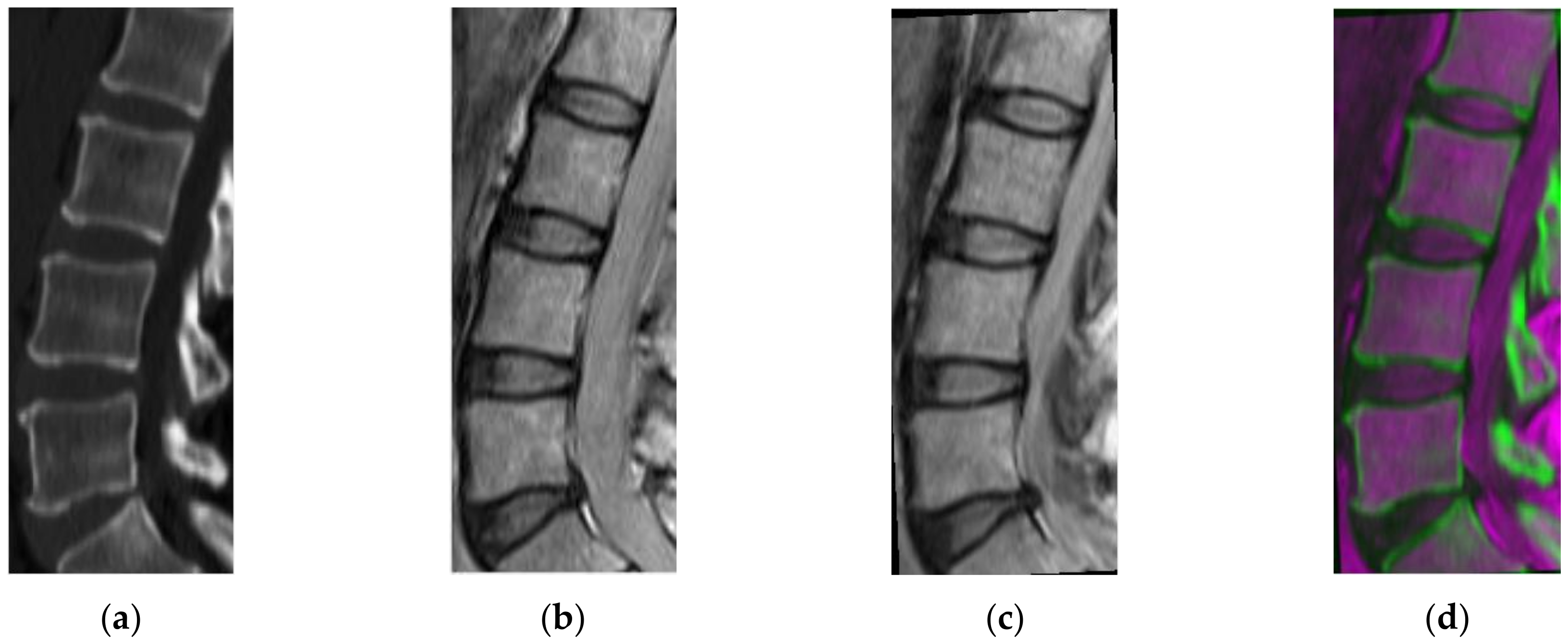
2.1. Geometric Transformation
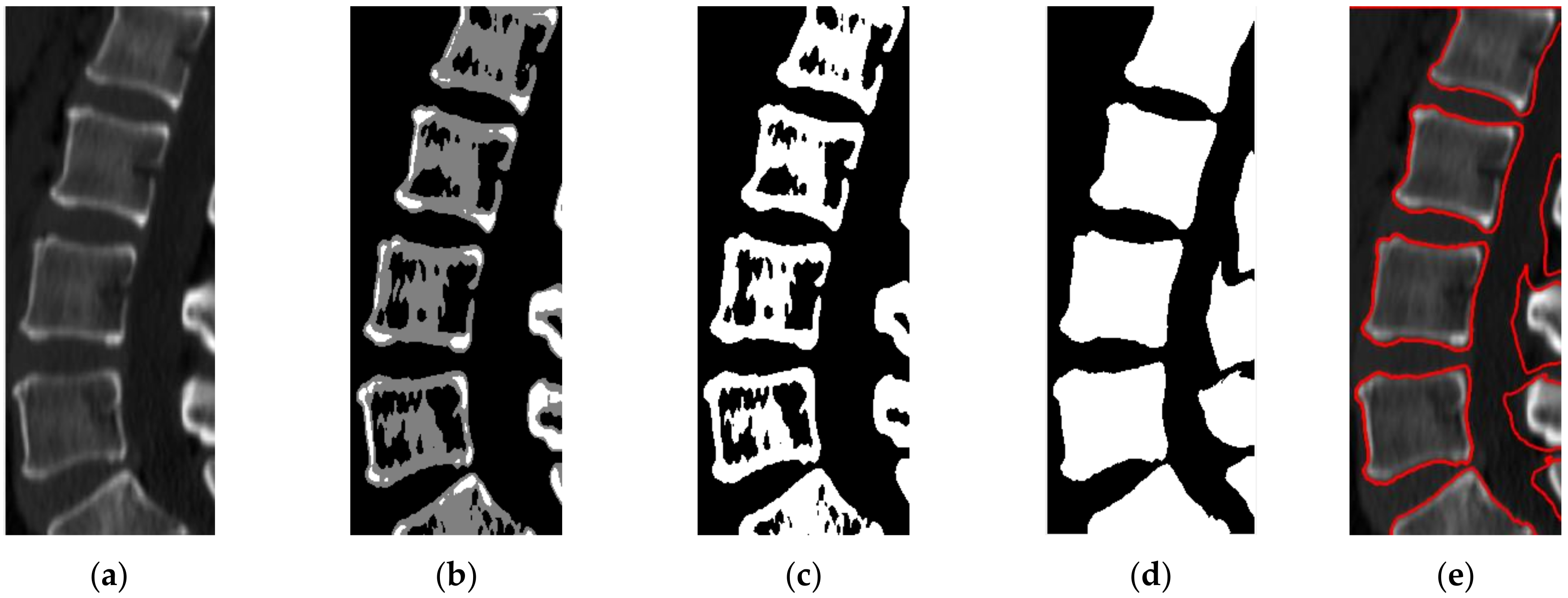
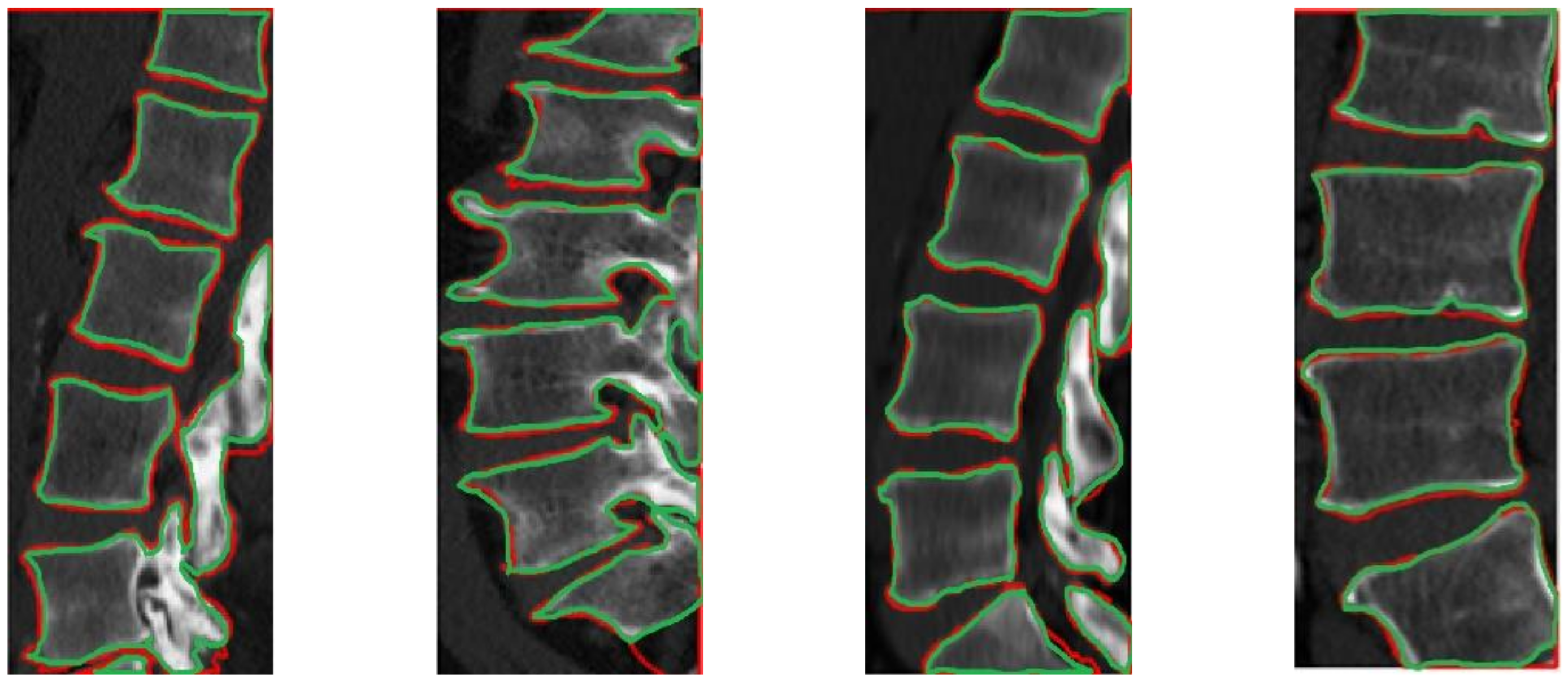
2.2. CT Segmentation for Vertebral Boundary Extraction
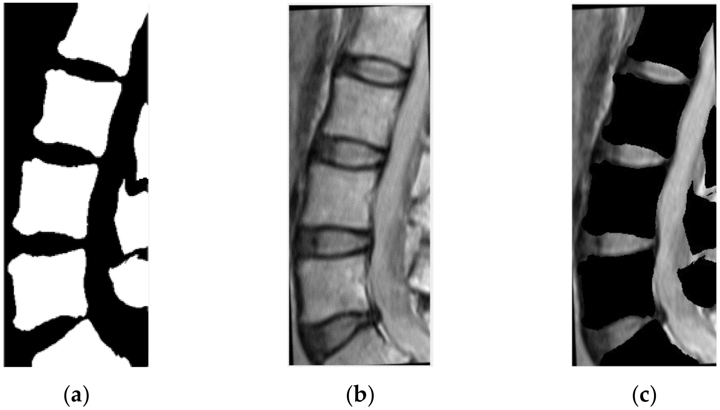
2.3. Vertebral Region Projection on MRI
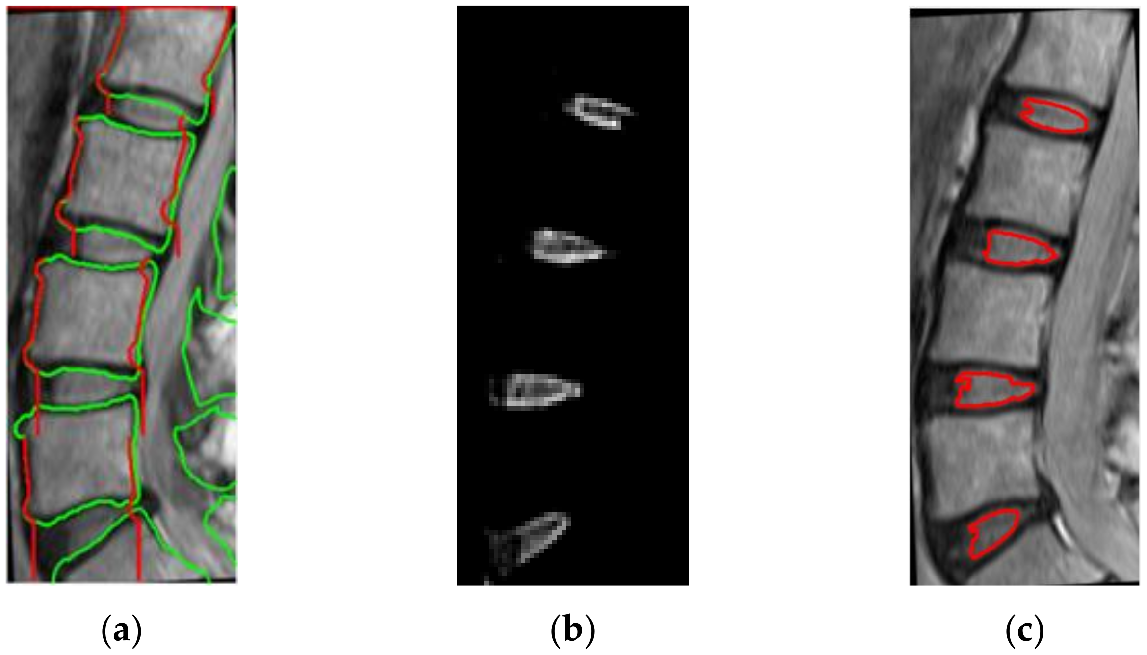
2.4. IVD Localization
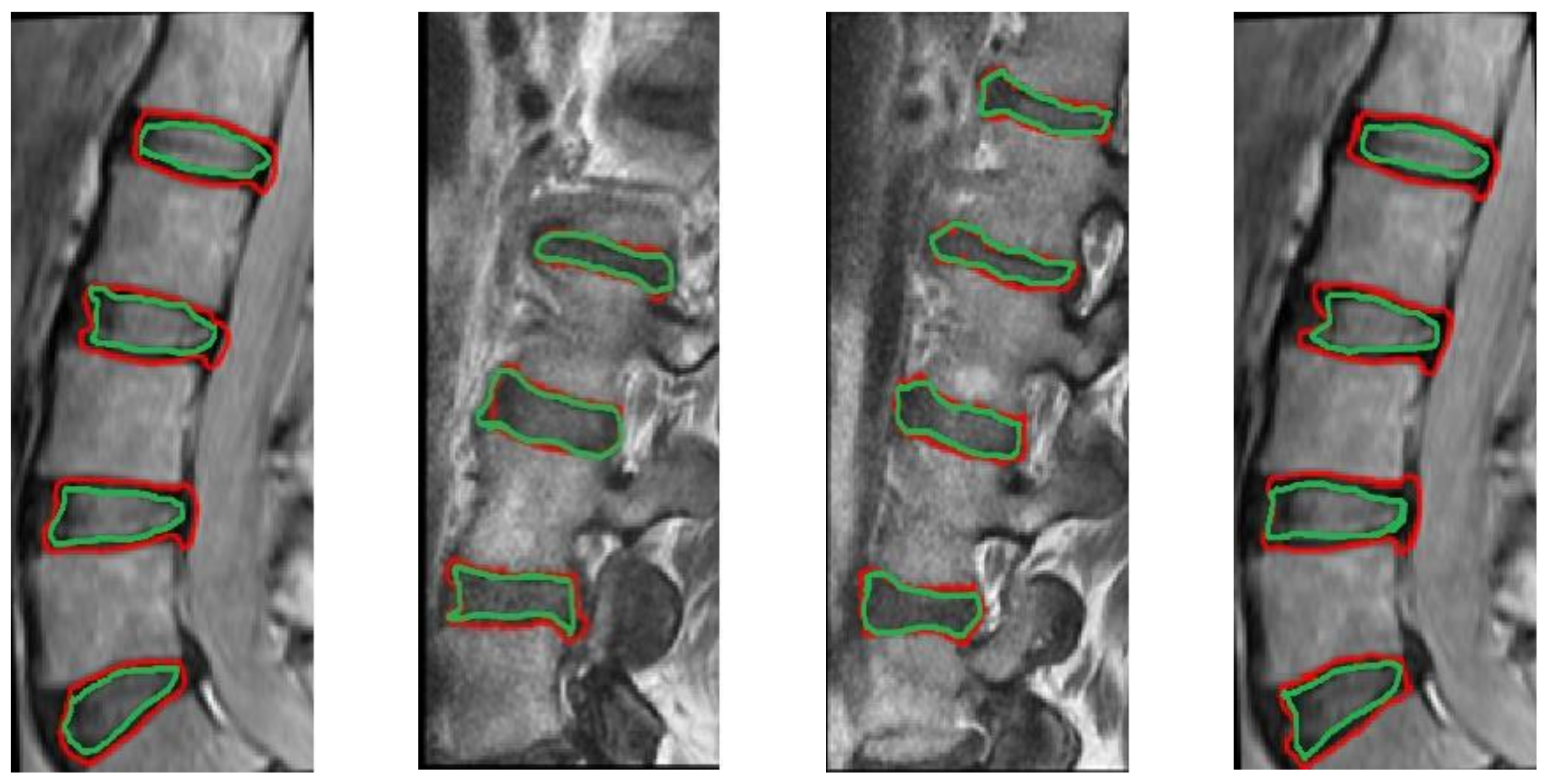
2.5. CT/MRI-Based Segmentation for IVD Boundary Extraction
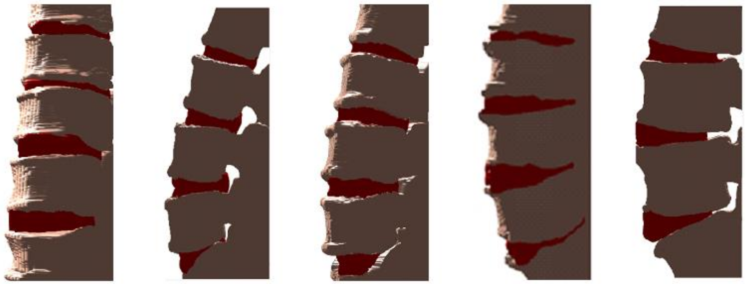
2.6. CT/MRI Image Fusion
3. Experimental Evaluation
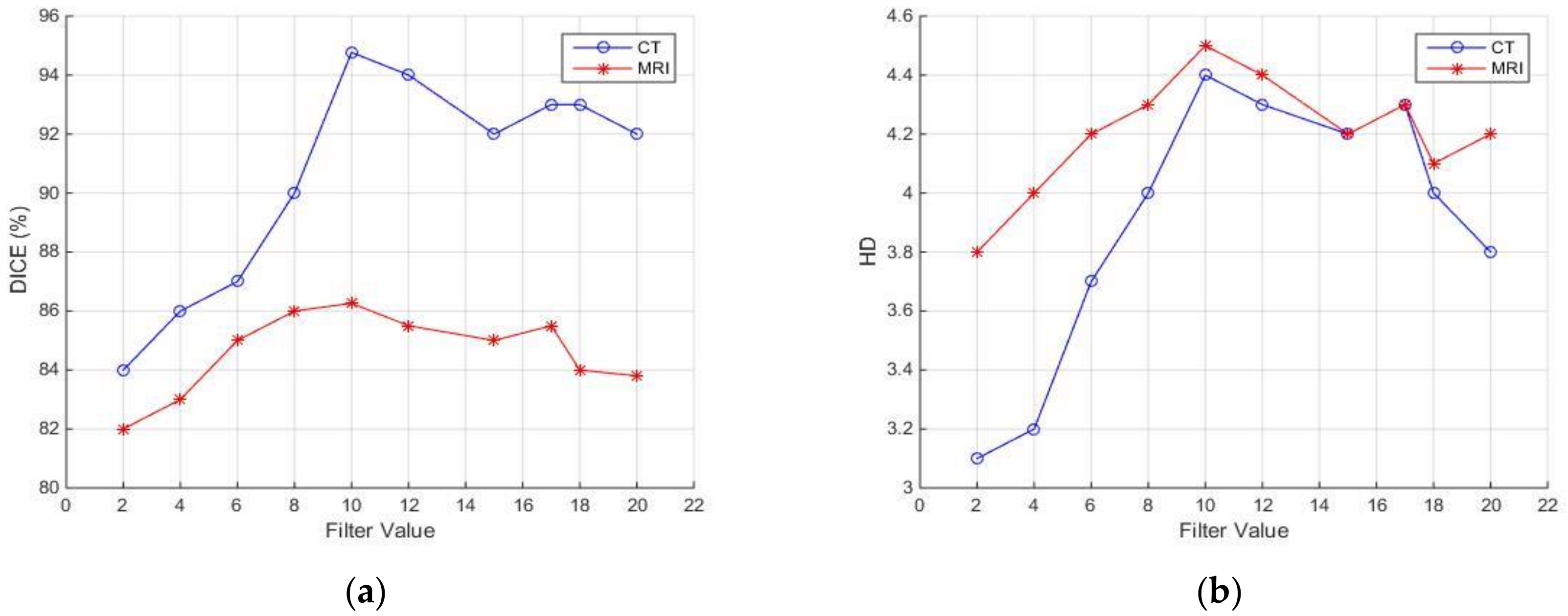
3.1. Evaluation Metrics
3.2. Results and Discussion
4. Conclusions
Author Contributions
Funding
Conflicts of Interest
References
- Oktay, A.; Akgul, A. Simultaneous localization of lumbar vertebrae and intervertebral discs with SVM-based MRF. IEEE Trans. Biomed. Eng. 2013, 60, 2375–2383. [Google Scholar] [CrossRef] [PubMed]
- Emch, T.; Modic, M. Imaging of lumbar degenerative disk disease: History and current state. Skelet. Radiol. 2011, 40, 1175–1189. [Google Scholar] [CrossRef] [PubMed]
- Huang, J.; Jian, F.; Wu, H.; Li, H. An improved level set method for vertebra CT image segmentation. Biomed. Eng. Online 2013, 12, 48. [Google Scholar] [CrossRef] [PubMed] [Green Version]
- Castro-M, I.; Pozo, J.M.; Pereañez, M.; Lekadir, K.; Lazary, A.; Frangi, A.F. Statistical interspace models (SIMs): Application to robust 3D spine segmentation. Trans. Med. Imaging 2015, 34, 1663–1675. [Google Scholar] [CrossRef] [PubMed]
- Zheng, G.; Chu, C.; Belavý, D.L.; Ibragimov, B.; Korez, R.; Vrtovec, T.; Hutt, H.; Everson, R.; Meakin, J.; Andrade, I.L.; et al. Evaluation and comparison of 3D intervertebral disc localization and segmentation methods for 3D T2 MR data: A grand challenge. Med. Image Anal. 2017, 35, 327–344. [Google Scholar] [CrossRef] [Green Version]
- Zheng, Y.; Nixon, M.S.; Allen, R. Automated segmentation of lumbar vertebrae in digital videofluoroscopic images. IEEE Trans. Med. Imag. 2004, 23, 45–52. [Google Scholar] [CrossRef]
- Peng, Z.; Zhong, J.; Wee, W.; Lee, J.H. Automated vertebra detection and segmentation from the whole spine MR images. In Proceedings of the IEEE-EMBC, Shanghai, China, 1–4 September 2005; pp. 2527–2530. [Google Scholar]
- Schmidt, S.; Kappes, J.; Bergtholdt, M.; Pekar, V.; Dries, S.; Bystrov, D.; Schnörr, C. Spine detection and labeling using a parts-based graphical model. In Proceedings of the IPMI, Kerkrade, The Netherlands, 2–6 July 2007; Volume 20, pp. 122–133. [Google Scholar]
- Corso, J.J.; Alomari, R.S.; Chaudhary, V. Lumbar disc localization and labeling with a probabilistic model on both pixel and object features. In Proceedings of the MICCAI, New York, NY, USA, 6–10 September 2008; Volume 11, pp. 202–210. [Google Scholar]
- Alomari, R.S.; Corso, J.; Chaudhary, V. Labeling of lumbar discs using both pixel and object-level features with a two-level probabilistic model. IEEE Trans. Med. Imaging 2011, 30, 1–10. [Google Scholar] [CrossRef]
- Stern, D.; Likar, B.; Pernus, F.; Vrtovec, T. Automated detection of spinal centrelines, vertebral bodies and intervertebral discs in CT and MR images of lumbar spine. Phys Med. Biol. 2010, 55, 247–264. [Google Scholar] [CrossRef]
- Donner, R.; Langs, G.; Micusik, B.; Bischof, H. Generalized sparse MRF appearance models. Image Vis. Comput. 2010, 28, 1031–1038. [Google Scholar] [CrossRef]
- Kelm, M.B.; Wels, M.; Zhou, K.S.; Seifert, S.; Suehling, M.; Zheng, Y.; Comaniciu, D. Spine detection in CT and MR using iterated marginal space learning. Med. Image Anal. 2013, 17, 1283–1292. [Google Scholar] [CrossRef]
- Chevrefils, C.; Cheriet, F.; Grimard, G.; Aubin, C.E. Watershed segmentation of intervertebral disk and spinal canal from MRI images. In Proceedings of the ICIAR LNCS, Montreal, QC, Canada, 22–24 August 2007; pp. 1017–1027. [Google Scholar]
- Chevrefils, C.; Farida, C.; Aubin, C.E.; Grimad, G. Texture analysis for automatic segmentation of intervertebral disks of scoliotic spines from MR images. IEEE Trans. Inf. Technol. Biomed. 2009, 13, 608–620. [Google Scholar] [CrossRef] [PubMed]
- Michopoulou, S.; Costaridou, L.; Panagiotopoulos, E. Atlas-based segmentation of degenerated lumbar intervertebral discs from MR images of the spine. IEEE Trans. Biomed. Eng. 2009, 56, 2225–2231. [Google Scholar] [CrossRef] [PubMed]
- Neubert, A.; Fripp, J.; Engstrom, C.; Schwarz, R.; Lauer, L.; Salvado, O.; Crozier, S. Automated detection, 3D segmentation and analysis of high resolution spine MR images using statistical shape models. Phys. Med. Biol. 2012, 57, 8357–8376. [Google Scholar] [CrossRef]
- Neubert, A.; Fripp, J.; Chandra, S.S.; Engstrom, C.; Crozier, S. Automated intervertebral disc segmentation using probabilistic shape estimation and active shape models. In Proceedings of the MICCAI Workshop & Challenge on Computational Methods and Clinical Applications for Spine Imaging, Munich, Germany, 5–9 October 2015; pp. 144–151. [Google Scholar]
- Carballido, G.J.; Belongie, S.J.; Majumdar, S. Normalized cuts in 3D for spinal MRI segmentation. IEEE Trans. Med. Imaging 2004, 23, 36–44. [Google Scholar] [CrossRef] [PubMed] [Green Version]
- Huang, S.Y.; Chu, S.; Lai, S.H.; Novak, C.L. Learning-based vertebra detection and iterative normalized cut segmentation for spinal MRI. IEEE Trans. Med. Imaging 2009, 28, 1595–1605. [Google Scholar] [CrossRef] [PubMed]
- Ali, A.M.; Aslan, A.S.; Farag, A.A. Vertebral body segmentation with prior shape constraints for accurate BMD measurements. Comput. Med. Imaging Graph. 2014, 38, 586–595. [Google Scholar] [CrossRef] [PubMed]
- Ayed, I.B.; Punithakumar, K.; Garvin, G.J.; Romano, W.M.; Li, S. Graph cuts with invariant object-interaction priors: Application to intervertebral disc segmentation. In Proceedings of the IPMI, Kloster Irsee, Germany, 3–8 July 2011; pp. 221–232. [Google Scholar]
- Law, M.; Tay, K.; Leung, A.; Garvin, G.; Li, S. Intervertebral disc segmentation in MR images using anisotropic oriented flux. Med. Image Anal. 2013, 17, 43–61. [Google Scholar] [CrossRef] [PubMed]
- Zhan, Y.; Maneesh, D.; Harder, M.; Zhou, X. Robust MR spine detection using hierarchical learning and local articulated model. In Proceedings of the MICCAI, Nice, France, 1–5 October 2012; Volume 1, pp. 141–148. [Google Scholar]
- Glocker, B.; Feulner, J. Automatic localization and identication of vertebrae in arbitrary field-of-view CT scans. In Proceedings of the MICCAI, Nice, France, 1–5 October 2012; pp. 590–598. [Google Scholar]
- Glocker, B.; Zikic, D.; Konukoglu, E. Vertebrae localization in pathological spine CT via dense classification from sparse annotations. In Proceedings of the MICCAI, Nagoya, Japan, 22–26 September 2013; pp. 262–270. [Google Scholar]
- Andrade, I.L.; Glocker, B. Complementary classification forests with graph-cut refinement for IVD localization and segmentation. In Proceedings of the MICCAI Workshop & Challenge on Computational Methods and Clinical Applications for Spine Imaging, Munich, Germany, 5–9 October 2015. [Google Scholar]
- Glocker, B.; Konukoglu, E.; Haynor, D. Random forests for localization of spinal anatomy. In Medical Image Recognition, Segmentation and Parsing: Methods, Theories and Applications; Academic Press: Orlando, FL, USA, 2016; pp. 94–110. [Google Scholar]
- Wang, C.; Forsberg, D. Segmentation of intervertebral discs in 3D MRI data using multi-atlas based registration. In Proceedings of the MICCAI Workshop & Challenge on Computational Methods and Clinical Applications for Spine Imaging, Munich, Germany, 5–9 October 2015; pp. 101–110. [Google Scholar]
- Korez, R.; Ibragimov, B.; Likar, B.; Pernus, F.; Vrtovec, T. Deformable model-based segmentation of intervertebral discs from MR spine images by using the SSC descriptor. In Proceedings of the MICCAI Workshop & Challenge on Computational Methods and Clinical Applications for Spine Imaging, Munich, Germany, 5–9 October 2015; pp. 111–118. [Google Scholar]
- Chen, C.; Belavy, D.; Yu, W.; Chu, C.; Armbrecht, G.; Bansmann, M.; Felsenberg, D.; Zheng, G. Localization and segmentation of 3D intervertebral discs in MR images by data driven estimation. IEEE Trans. Med. Imaging 2015, 34, 1719–1729. [Google Scholar] [CrossRef]
- Cai, Y.; Osman, S.; Sharma, M.; Landis, M.; Li, S. Multi-modality vertebra recognition in artbitrary view using 3D deformable hierarchical model. IEEE Trans. Med. Imaging 2015, 34, 1676–1693. [Google Scholar] [CrossRef]
- Suzani, A.; Seitel, A.; Liu, Y.; Fels, S.; Rohling, N.R.; Abolmaesumi, P. Fast automatic vertebrae detection and localization in pathological CT scans—A deep learning approach. In Proceedings of the MICCAI, Munich, Germany, 5–9 October 2015. [Google Scholar]
- Chen, H.; Shen, C.; Qin, J. Automatic localization and identification of vertebrae in spine CT via a joint learning model with deep neural network. In Proceedings of the MICCAI, Munich, Germany, 5–9 October 2015; Volume 1, pp. 515–522. [Google Scholar]
- Chen, H.; Dou, Q.; Wang, X.; Heng, P.A. Deepseg: Deep segmentation network for intervertebral disc localization and segmentation. In Proceedings of the MICCAI Workshop & Challenge on Computational Methods and Clinical Applications for Spine Imaging, Munich, Germany, 5–9 October 2015. [Google Scholar]
- Styner, M.; Brechbühler, C.; Székely, G.; Gerig, G. Parametric estimate of intensity inhomogeneities applied to MRI. IEEE Trans. Med. Imaging 2000, 19, 153–165. [Google Scholar] [CrossRef]
- Wells, W.M.; Viola, P.; Atsumi, H.; Nakajima, S.; Kikinis, R. Multi-modal volume registration by maximization of mutual information. Med. Image Anal. 1996, 1, 35–51. [Google Scholar] [CrossRef]
- Otsu, N. A threshold selection method from gray-level histograms. IEEE Trans. Syst. Man. Cyber. 1979, 9, 62–66. [Google Scholar] [CrossRef] [Green Version]
- Chan, T.F.; Vese, L.A. Active Contours Without Edges. IEEE Trans. Image Process. 2001, 10, 266–277. [Google Scholar] [CrossRef] [Green Version]
- Saleh, H.; Nordin, M.J. Improving diagnostic viewing of medical images using enhancement algorithms. J. Comput. Sci. 2011, 7, 1831–1838. [Google Scholar]
- Taha, A.A.; Hanbury, A. Metrics for evaluation 3D medical image segmentation: Analysis, selection, and tool. BMC Med. Imaging 2015, 15, 29. [Google Scholar] [CrossRef] [Green Version]
- Huttenlocher, D.; Klanderma, G.; Rucklidge, W. Comparing Images Using the Hausdorff Distance. IEEE Trans. Pattern Anal. Mach. Intell. 1993, 15, 850–863. [Google Scholar] [CrossRef] [Green Version]


| Method | Advantages | Limitations | Average Run Time | |
|---|---|---|---|---|
| CT | Huang [3] | Segment images with intensity inhomogeneity and blurry discontinuous boundaries. | Time depends on iterations, 0.7–20.2 s, 2.79 GHz Matlab | |
| Isaac [4] | A model of the interspace between objects to guaranteed that the shapes are not deformed. | Requires the manual selection of the IVD center. | 50 s per vertebra, 2.4 GHz C++ | |
| MR | Lopez Andrade and Glocker [27] | Globally optimal segmentation with learned likelihood. | L5-S1 disc should be present. Requires training. | 3 min, 3.5 GHz 4-cores Python and C++. |
| Wang and Forsberg [29] | Highly parallelizable. | Complexity depends on the number of atlases. Problems in the segmentation of structures deviating from atlases. | 8.5 min, 3.2 GHz 4-cores Matlab and Cuda. | |
| Chen [35] | Leveraging flexible 3D convolution kernels. Fast volume-to-volume classification. | Computationally intensive. Memory cost is proportional to image resolution. | 3.1 s, 2.5 GHz 4-cores Python. | |
| Korez [30] | Computationally efficient and robust. | Computational complexity proportional to the number of voxels used for training. Problems in the presence of severe pathologies and cropped image parts. | 5 min, 3.2 GHz 4-cores C ++ and Matlab. |
| Method | Mean DSC (%) ± SD | Mean HD (mm) ± SD |
|---|---|---|
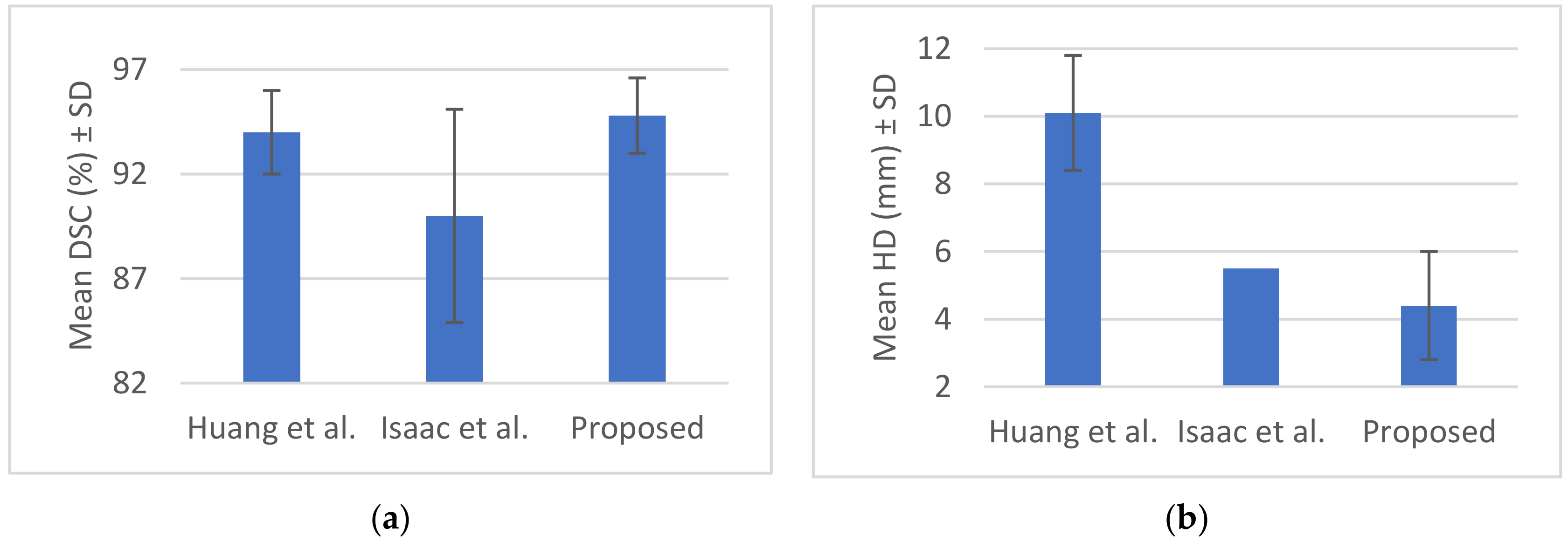
| Huang et al. [3] | 94.0 ± 2.0 | 10.1 ± 1.7 |
| Isaac et al. [4] | 90.0 ± 5.1 | 5.5 |
| Proposed | 94.8 ± 1.8 | 4.4 ± 1.6 |
| Method | Mean DSC (%) ± SD | Mean HD (mm) ± SD |
|---|---|---|
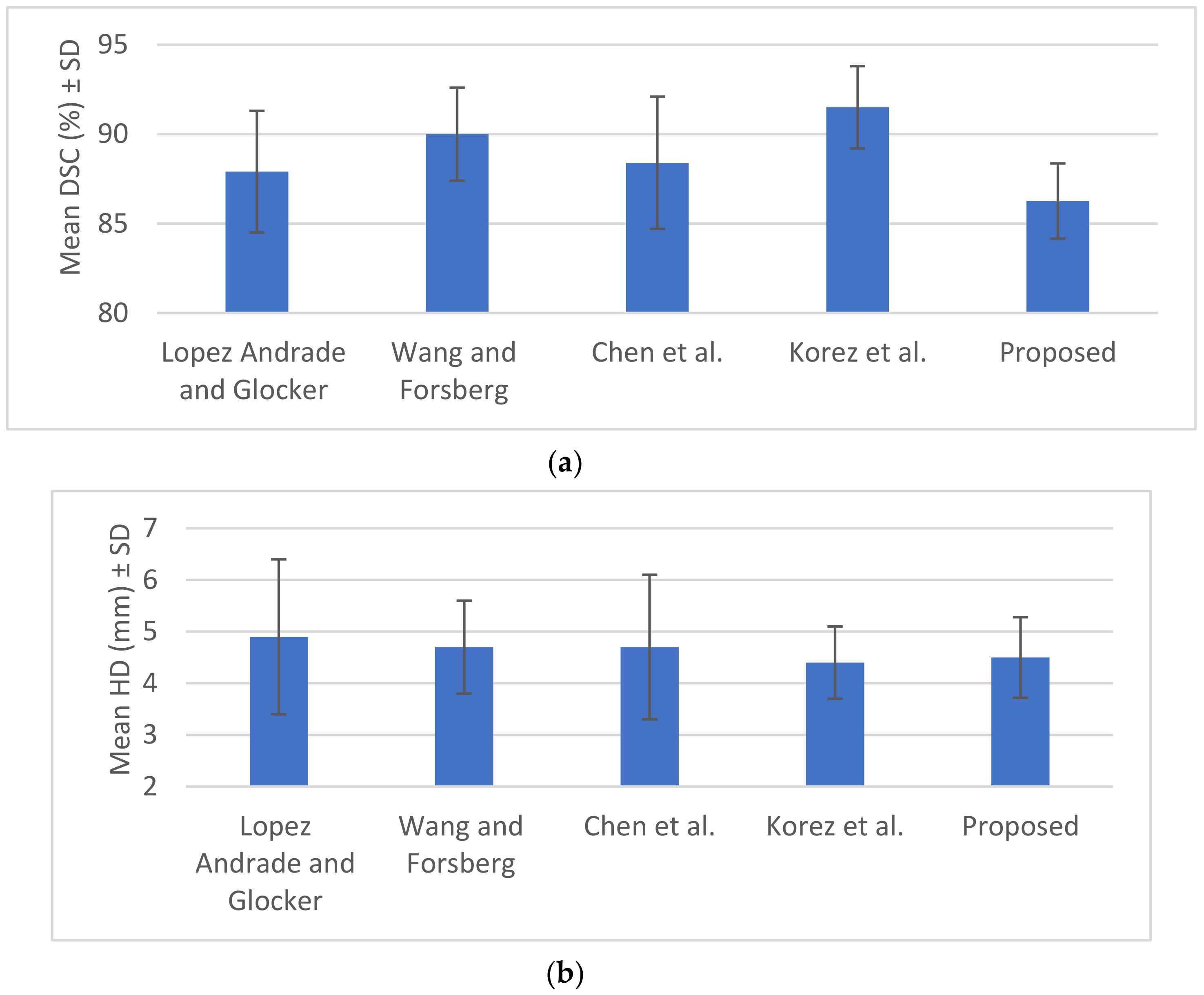
| Lopez Andrade and Glocker [27] | 87.9 ± 3.4 | 4.9 ± 1.5 |
| Wang and Forsberg [29] | 90.0 ± 2.6 | 4.7 ± 0.9 |
| Chen et al. [35] | 88.4 ± 3.7 | 4.7 ± 1.4 |
| Korez et al. [30] | 91.5 ± 2.3 | 4.4 ± 0.7 |
| Proposed | 86.26 ± 2.1 | 4.5 ± 0.78 |
© 2020 by the authors. Licensee MDPI, Basel, Switzerland. This article is an open access article distributed under the terms and conditions of the Creative Commons Attribution (CC BY) license (http://creativecommons.org/licenses/by/4.0/).
Share and Cite
Liaskos, M.; Savelonas, M.A.; Asvestas, P.A.; Lykissas, M.G.; Matsopoulos, G.K. Bimodal CT/MRI-Based Segmentation Method for Intervertebral Disc Boundary Extraction. Information 2020, 11, 448. https://0-doi-org.brum.beds.ac.uk/10.3390/info11090448
Liaskos M, Savelonas MA, Asvestas PA, Lykissas MG, Matsopoulos GK. Bimodal CT/MRI-Based Segmentation Method for Intervertebral Disc Boundary Extraction. Information. 2020; 11(9):448. https://0-doi-org.brum.beds.ac.uk/10.3390/info11090448
Chicago/Turabian StyleLiaskos, Meletios, Michalis A. Savelonas, Pantelis A. Asvestas, Marios G. Lykissas, and George K. Matsopoulos. 2020. "Bimodal CT/MRI-Based Segmentation Method for Intervertebral Disc Boundary Extraction" Information 11, no. 9: 448. https://0-doi-org.brum.beds.ac.uk/10.3390/info11090448