Identification of Social Aspects by Means of Inertial Sensor Data


Department of Physics, Informatics and Mathematics, University of Modena and Reggio Emilia, 41125 Modena MO, Italy
*
Author to whom correspondence should be addressed.
Information 2020, 11(11), 534; https://0-doi-org.brum.beds.ac.uk/10.3390/info11110534
Submission received: 5 October 2020
/
Revised: 6 November 2020
/
Accepted: 11 November 2020
/
Published: 17 November 2020
(This article belongs to the Special Issue The Integration of Digital and Social Systems)
Abstract
:Today’s applications and providers are very interested in knowing the social aspects of users in order to customize the services they provide and to be more effective. Among the others, the most frequented places and the paths to reach them are information that turns out to be very useful to define users’ habits. The most exploited means to acquire positions and paths is the GPS sensor, however it has been shown how leveraging inertial data from installed sensors can lead to path identification. In this work, we present a Computationally Efficient algorithm to Reconstruct Vehicular Traces (CERT), a novel algorithm which computes the path traveled by a vehicle using accelerometer and magnetometer data. We show that by analyzing data obtained through the accelerometer and the magnetometer in vehicular scenarios, CERT achieves almost perfect identification for medium and small sized cities. Moreover, we show that the longer the path, the easier it is to recognize it. We also present results characterizing the privacy risks depending on the area of the world, since, as we show, urban dynamics play a key role in the path detection.
1. Introduction
In our everyday life, we leverage a lot of services that support us in several activities. Such services are more effective if they take into consideration the information of the user that exploits them in order to provide a more customized support. To this end, applications and providers are interested in getting information about the social aspects of users. Two of these social aspects are the most frequented places and the paths of a user. In fact, the most frequented places represent where the users spend their time and can be useful to guess their interests and their relationships; the path of the users can be exploited to build the dynamism of their social life. GPS is the most exploited means to get positions and paths, even if it has some limitations due to the possible variation of the exploited data, but there are also other means as reported in the literature and in this paper. One way is to exploit Inertial Measurement Units (IMUs), which are nowadays present in a multitude of devices, including smartphones, tablets and cars. Leveraging the data obtained from these sensors it is possible to provide rich, context-aware services depending on the scenario and on the objective of the user. Focusing our analysis on the vehicular scenario, we show that by using accelerometers and magnetometers, it is possible to determine the distance traveled by the devices thanks to the former, and the orientation of the road in which the device is traveling thanks to the latter. Systems such as the one used in this study are called Dead Reckoning System (DRS), in which inertial sensors are analyzed and a trajectory is eventually computed. However, only relying on DRS would easily lead to large errors, particularly in vehicular scenarios in which distances can be considerably long, hence systems presented in this domain typically leverage the use of additional data to compensate the error [1,2].
The main focus of this work is to present a novel approach to trace the user’s position without relying on GPS information; our proposal exploits only inertial sensors such as accelerometers and magnetometers, which typically can be used freely with no specific permissions also in mobile applications. The proposed approach is based on Computationally Efficient algorithm to Reconstruct Vehicular Traces (CERT), a novel algorithm which matches data obtained from accelerometers and magnetometers to real roads, does not need any GPS readings, and corrects the accumulated errors from the DRS through publicly available vehicular maps, obtained through OpenStreetMap (http://www.openstreetmap.org). The main objective of CERT is to perform the detection fast, by computing in advance possible paths of different lengths in the area of interest, to make the detection quicker when the path data are available. Generally the detection is performed analyzing the similarity from the computed traces against real world data in an iterative way [2,3,4]. However, this process can take quite a long amount of computation time, particularly in large maps where the urban road dynamics may be complex, hence with a possibly large number of paths. Thus in this work we focus on the computational efficiency of the algorithm. CERT is based on graph theory, and builds in advance N-clique subsets, where N is the length of the path to be recognized. Though the clique problem is known to be NP-hard, it is performed only once for the area in which the recognition should take place. The computed cliques are then matched against data obtained from the IMU, much faster than going through the graph each time a new path has to be detected. Through our study we show that the detection of paths traveled with a car by a human being can indeed be recognized more efficiently through our proposal.
To extend our study to multiple cities and on longer road paths, we develop a custom simulator, which provides inertial sensors data for vehicles driving in a given road map. We then use such simulated data to run CERT, and match the sensor data on the map obtained from OpenStreetMap, showing to what extent it is possible to uniquely match paths on maps. In this case, our aim is to quantify the detection probability of a path in a large area such as a city, and uncover the role of the urban landscape in detecting the path traveled. Clearly, how similar roads and turns are in a city can vary the performance of the path identification. For instance, in small cities roads are more characteristic and unique, hence recognizing them would make the whole path recognition easier. Conversely, in large cities, which are built with longer roads and more similar turns, even recognizing the length of a road or the degrees of a turn would make the identification of the specific road more challenging.
We show that in most cities worldwide it is possible to uniquely identify paths with at least 10 turns, even in big cities with thousands of different roads. Given the current driving styles of individuals, it is safe to say that most of the driving journeys exceed this number of turns [5,6,7,8]. Moreover, we show that there exists a correlation between the detection probability and the area of the world in which the detection takes place. Continents such as Europe and Oceania are far more identifiable, while American countries exhibit more resilience to this approach, as the urban deployment resembles more a Manhattan grid, hence with turns and roads more similar among each other.
Of course, the exploitation of means different from GPS, for which the user is not asked to grant permission, introduces some privacy issues that must be taken into consideration [9]. We remark that the purpose of this paper is to introduce an approach alternative to GPS, however we will discuss them in the conclusions.
The rest of this paper is organized as follows: Section 2 presents related work from the literature; Section 3 presents the model we used in this study, based on graph theory; Section 4 discusses the algorithm we use to match different graphs; Section 5 presents the results of our study; Section 6 concludes this work.
2. Related Work
Applications and services based on context awareness have skyrocketed since the appearance of mobile devices. The ability to report the location of the user, or the activity they are performing, or the possibility to understand the environment in which the device is located is of paramount importance for most of novel applications.
Context aware computing means, for a computing system, being able to adapt its computation dependent on the context in which the device is located [10]. Context can be anything which can be used to characterize the situation of the device, such as the location, the activity, the neighbors and so on. For instance inertial sensors such as the accelerometer, gyroscope and the magnetometer, are used for the so-called Transportation Mode Detection (TMD), which is the ability to determine how the user is moving, whether they are standing still, driving a car, being on a train or walking [11,12,13]. Apart from inertial sensors, also GPS has been used in the past to assess the transportation mode of the user, though with an increased battery consumption and with mediocre results, particularly for those transportation modes which present similar speeds [14]. Many applications rely on this data to provide tailored, custom made reports about the user activity, and eventually provide a better quality of experience when using the mobile device. Detecting spatiotemporal patterns of traffic and mobility can also be useful to optimize services, such as the ones provided by cellular networks [15].
Inertial sensors have also been effectively used in Indoor navigation systems, due to the fact that GPS is highly inaccurate indoors [16]. Other possibilities also encompass the use of WiFi fingerprints, through which it is built a map at first, later used to match WiFi readings. Inertial sensors have also been employed for augmented reality [17,18], to better adapt to the users’ movements.
Another area closer to the scope of this work in which inertial sensors are actively used is DRS, which exploit data from the sensors to obtain the trajectory of the mobile device. A multitude of sensors can be used, ranging form accelerometers to determine linear acceleration, hence space, gyroscope to assess turns, magnetometers to determine the orientation, the barometer to account for altitude changes and many others [19,20]. Another technique used is that related to sporadic GPS corrections, particularly useful in urban canyons or whenever GPS accuracy is scarce [21,22]. Here, sensors may help to stabilize inaccurate GPS data, understanding whether the user is moving or not and with what speed. Reference [23] presents ACComplice, a system which shows how to track users whilst driving using only accelerometers.
Instead, fewer works can be found in which both DRS and road data are merged to raise the localization accuracy. Generally, inertial sensors are instead combined with other sources of information, such as WiFi fingerprints, Ultra Wide Band (UWB) and cellular systems, to increase the performance of the system or to increase the amount of information which can be inferred. This can be used also to build indoor maps [24,25], which may be obtained from OpenStreetMap such as [26,27] do. Data obtained from OpenStreetMap have been proved to be particularly useful in a multitude of different research scenarios. For instance, it has been leveraged to generate real vehicular traces, or to improve existing ones [28]. It also helps in vehicular navigation systems such as [29], where it is used to provide additional information to the human being. In general we can say that the data offer plenty of details, although certain cities offer richer and more precise data compared to others. This is directly related to the users which report measurements, since in some areas there are more of them recording the urban data, and some also report it with more precision.
Reference [3] shows how it is possible to track users when considering four different mobility types, which are walking, traveling on a train, driving and traveling on a plane. Their work shows that it is not necessary to pin-point the exact starting location of the user, similarly to CERT, as they only need an area in which the user may have traveled.
The work presented firstly in [4] and later extended in [2] shows that through magnetometers, accelerometers and gyroscopes, installed in COTS devices, it is possible to track users on vehicles, matching the movements with real maps. The authors too use graph theory, but they travel the graph for each route, assigning probabilities between paths in the graph and sensed measurements.
Compared to the aforementioned works, which focus mainly on how to carefully measure distances and angles, we focus instead on the algorithm which can be run to identify users based on such measurements. In particular compared to our previous work [30] we show how computationally it can be improved the offline traces reconstruction, by using graph theory and computing in advance subgraphs of the area of interest.
We summarize the literature in Table 1.
3. Graph Model
In this section we describe the model we use in this study, which is based on two graphs, one obtained from raw sensor measurements called , and the other which we name instead , downloaded from the OpenStreetMap Internet archive. The overarching idea of our approach is to find the best match of , so that raw measurements can be matched to a real road path. Moreover, does not change in a city, hence it can be computed before the attack takes place, making the matching of much faster. In the following sections we describe each of these graphs, starting with the definition of in Section 3.1. We then describe how we leverage and enrich the data through which is built in Section 3.2.
3.1. Construction
In this section we describe how we build , starting from raw sensor measurements. The methodology on how to collect samples and translate them into linear acceleration and orientation has already been studied in the literature [2,3], hence we focus our discussion on how we leverage this information to build . We assume that both the accelerometer and the magnetometer are already compensated for the orientation, thus they give the linear acceleration aligned with respect to the orientation and the direction of the car.
In each edge is defined with a length and an absolute angle , while each vertex represents a possible turn.
In order to build we perform two separate steps. The first one is devoted to identify road segments, and is described in Section 3.1.1, while the second step is carried out by a dead reckoning system, needed to compute the road segments lengths, and is detailed in Section 3.1.2.
3.1.1. Road Segments Identification
The task performed by the first step of our proposal is devoted to understand the number of road segments which have been traveled with the mobile device. Let be the raw measurement at time t, equal to , where is the measurement of the accelerometer at time t, while is instead the measurement of the magnetometer at time t. For the segment identification performed in this step, we only need , and to do so we compute the moving mean at time t, defined as
and also the corresponding moving variance defined similarly as
Let be a binary hypothesis representing whether we turned or not. More precisely
where is set to
which is basically the mean of the moving means computed through Equation (1). Each element of H is either 0 or 1. If at time t, then the car is not turning at that time, if instead we observe a 0 it means the car is turning at time t. Simplifying, a turn starts when we observe a transition , and ends when we face a transition.
It is then straightforward to build the vector , representing all the orientations at any given time t, where each element is defined as follows:
It is easy to see that when we do observe any turn at time t, then , as we do not consider measurements obtained from the magnetometer, while instead if , thus on a road segments and not during a turn, then .
3.1.2. Dead Reckoning System
We now detail the Dead Reckoning System (DRS) we leverage to estimate the length of each road segment.
We define the vector in which each element is computed as
It is easy to note, as before, that each element can be either 0 or , which is the orientation independent value of the accelerometer at time t.
Let be an array of time couples where with we have
and correspondingly
and in which each time i and is present at most once in a couple. In other words, each element represents the time at which the mobile device started to travel in a segment, and the instant in which it ended.
We can then calculate the total distance traveled over each road segment k, , as follows:
Through Equation (6) we compute the total length of each segment, accounting for the initial speed and the total acceleration computed in within the time during which the mobile device traveled along a given road segment. Clearly, this measurement starts at the beginning of a road segment and ends at the end of it.
We perform a similar operation also to compute the angle of the road segment, as follows:
which is basically the average angle between time i and time .
3.2. Definition
The graph is simply obtained by downloading the area of interest through OpenStreetMap. As we already stated, we do not need to know the starting position of the user as also [3] does, but we do assume to know the area in which the journey happens. However, there are no theoretical limits on the size of the area, which can be a neighborhood, a city or even a bigger region. The data returned from OpenStreetMap are very rich, and contains a lot of information in it. For our purposes, we strip all the data about vertices and edges we do not need, and keep only edge lengths and angles.
A final step needed on is to add all possible edges in which the mobile device traveled straight through a crossroad. More formally, given three nodes , and , and their respective edges and , we add the edge if
which means that their respective angles do not differ more than . Then we set
which is the mean of the two angles. The length obviously is
This step is needed since our model only accounts for different segments when the mobile device turns, changing its orientation. Hence, if the user is driving on a straight road, passing through crossroads, our framework would match the segment to a unique, straight segment. However in we would not have the possibility to match such a long segment. Instead, by adding further edges according to the segments angles, we keep in both the original connections and also those which the user would travel if driving straight at a crossroad.
3.3. Complexity of CERT
As we have shown the main steps of CERT, we now discuss its complexity. The time needed to obtain is only related to the download speed. Instead, enhancing the graph requires to examine each node, and for each node adding the required roads. Hence its complexity is , where N is the number of nodes in .
The clique problem is instead known to be NP-complete, however we remark that the step is performed only once, hence although onerous, it can be computed in advance. We will show in Section 5.3 experiments with timings, which assess practically the time needed to perform this step.
Finally the segments matching is again linear, as it needs to examine each subgraph found by the clique operation. Hence let M be the number of subgraphs found, and L the length of the path, the complexity of this step is . Again in Section 5.3 we show quantitative measures on the timing and number of subgraphs found in different cities.
4. Segments Matching
In this section, we describe the last step of CERT, to match sensor data to road segments. The overarching idea of this step is to find the subgraph which is the most similar to .
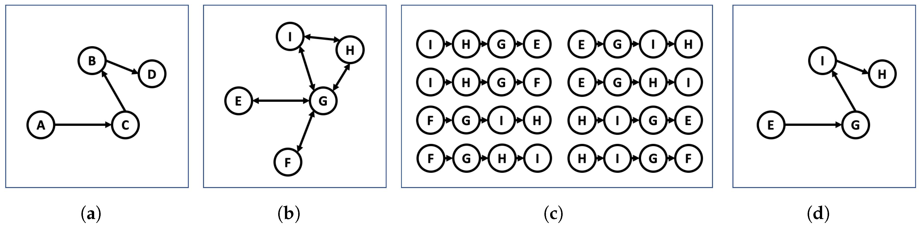
We summarize our idea in Figure 1, where we show the four steps of the CERT algorithm. At first we compute from the raw data obtained from the inertial sensors, as we described in Section 3.1. Then is downloaded from the internet as we explained in Section 3.2, and we find all the possible subgraphs with the same number of nodes as . Eventually, we select the one which matches better , as we will explain in this section.
At first, we find all the subgraphs where any , such that
The equivalence is defined between two generic graphs and , whose edges are defined as a couple containing the length and the angle of edge. More formally the edges are defined as
and
Hence the equivalence is defined as follows:
Basically matches all the graphs which differ at most and from the original graph for all the edges, both in terms of the length of edge and its orientation. By applying Equivalence (11) to our scenario we can define the following:
where n is the total number of paths we want to find. In case we want a perfect detection of the path obviously . However, this would require a high computation cost, since it would require to try and test all the possible values of and until the correct number of chart is found. Hence, in the following section we describe how to eventually reduce the number of matching graphs only to those more similar to . We also highlight the fact that may have some streets collected differently than what they are in reality, and is built with sensor data, hence with possible noise hence imperfect road lengths and turns. The and parameters may also be used to take into account this, as increasing them mitigates the problem of graph discrepancies, while reducing them requires a more accurate graph definition.
Comparing Graphs
With the technique described in the previous section we end up with a possibly large number of subgraphs which match the structure of , hence we need to find the one which is more similar to it. Since each graph and have the same structure, we compare node-to-node and edge-to-edge, to find differences and similarities.
We define the matrix related to graph , representing road angles, whose elements are
Each element is defined taking into account the difference in angle between edge and edge
We then define the matrix related to graph , representing edges’ length, whose elements are
The differences between graphs and are computed according to the following two equations:
where ∘ is the Hadamard product [31].
We then consider and and we combine them as
where , and are determined taking into account . Clearly the value of and has a strong influence on the performance of our system. Putting them equal among each other means we care about edges and node at the same weight. Increasing alpha gives more importance to node angles, while decreasing the importance of the edges length, and increasing has instead the opposite effect.
To determine the appropriate values of and we start from the OSM graph . The general idea is that if we have many similar edge lengths, then an error on should be weighted less, as it may be more probable, while instead if edges are more distinct, it is harder to get measurements wrong, hence the error should be weighted more. A practical example is the difference between roads in different continents, which are built differently considering the urban landscape of cities. We show in Figure 2 the Probability Density Function (PDF) concerning the distribution of the edges lengths and road angles in several worldwide cities. What Figure 2a highlights is the fact that in some cities’ roads are more similar than in others, and so do also the road angles. If we take for instance the case of North America, we see that there are higher densities around 90, 180, 270 and 360 degrees, which are due to the Manhattan grid deployment. In other continents road angles are more evenly distributed. The road length distribution, shown in Figure 2b, highlights instead that road lengths are more similar among continents.
In detail, and are defined as follows. We analyze primarily road angles, as their measurement is more stable than road lengths. This is simply due to the fact that for straight road segments, the value of the magnetometer is stable. Instead, road lengths are computed accounting for acceleration along the segment, which may have more variations leading to larger errors. We will provide performance evidence of this in Section 5.2.
To perform this step, we normalize all road angles values to be , hence is computed as the variance of the road angles, as follows:
where N is the total number of road angles, is the average and is the i-th value. Accordingly:
In Figure 2c we plot the results of a study which evaluates the values of and for several cities in Europe and in North America. We omit other continents as they show similar results to Europe, as also confirmed by the two previous charts, and would also make the chart less readable. More than 20,000 cities of different sizes have been evaluated, and the results highlight that North American cities tend to have lower values compared to European cities, meaning that is higher. This happens as North American cities have angles with more similar values, hence reducing the variance of the data. This will eventually result in a lower weight given on angles errors, as we formalized in Equation (15).
We summarize our model and algorithm steps in Figure 3. We note that although pictured sequentially, the download of and the clique operation can be performed in advance and stored in memory.
5. Evaluation
In this section we provide numerical results of our framework. We are mainly interested in understanding how precise it can be the recognition of a path recorded using only inertial sensors, and whether it would be possible to detect it among a urban road map.
Section 5.1 highlights the details of the simulator we built, to perform a wide analysis on simulated data, which enables the validation of the proposed framework in different cities with changing urban landscapes. Section 5.2 shows the results of our evaluation, and finally Section 5 analyzes the CERT performance.
5.1. Simulator
To perform a wider analysis of our framework, and on varying urban landscapes with different road segments, we developed a simulator written in Python which generates random paths within a city, collects inertial data from a simulated mobile device inside a car, and passes such data to our framework.
At first, we select a map on which we want to simulate data and perform our analysis. This can be either a city, a smaller scenario or even an entire country. This area is then queried to OpenStreetMap and downloaded in the form of a graph, where each edge is a road segment, and each node is a connection between road segments.
We are then able to choose a set of parameters through which we can configure the simulation, such as the orientation of the device, the noise on the accelerometer and on the magnetometer, the number of paths to be simulated and their lengths. These parameters are fed to the simulator, which randomly picks a starting point and an ending point and generates the shortest path between them until a path of the desired size is found. For each road segment of the path found it is then generated a simulated measure accounting for the noise of the device. As we wrote in Section 3.2, . Let be the graph obtained through the simulator. For each we perturbate its corresponding value defining the length as
where is a normal distribution with mean and variance . Accordingly, we perform the same operation for the road angles
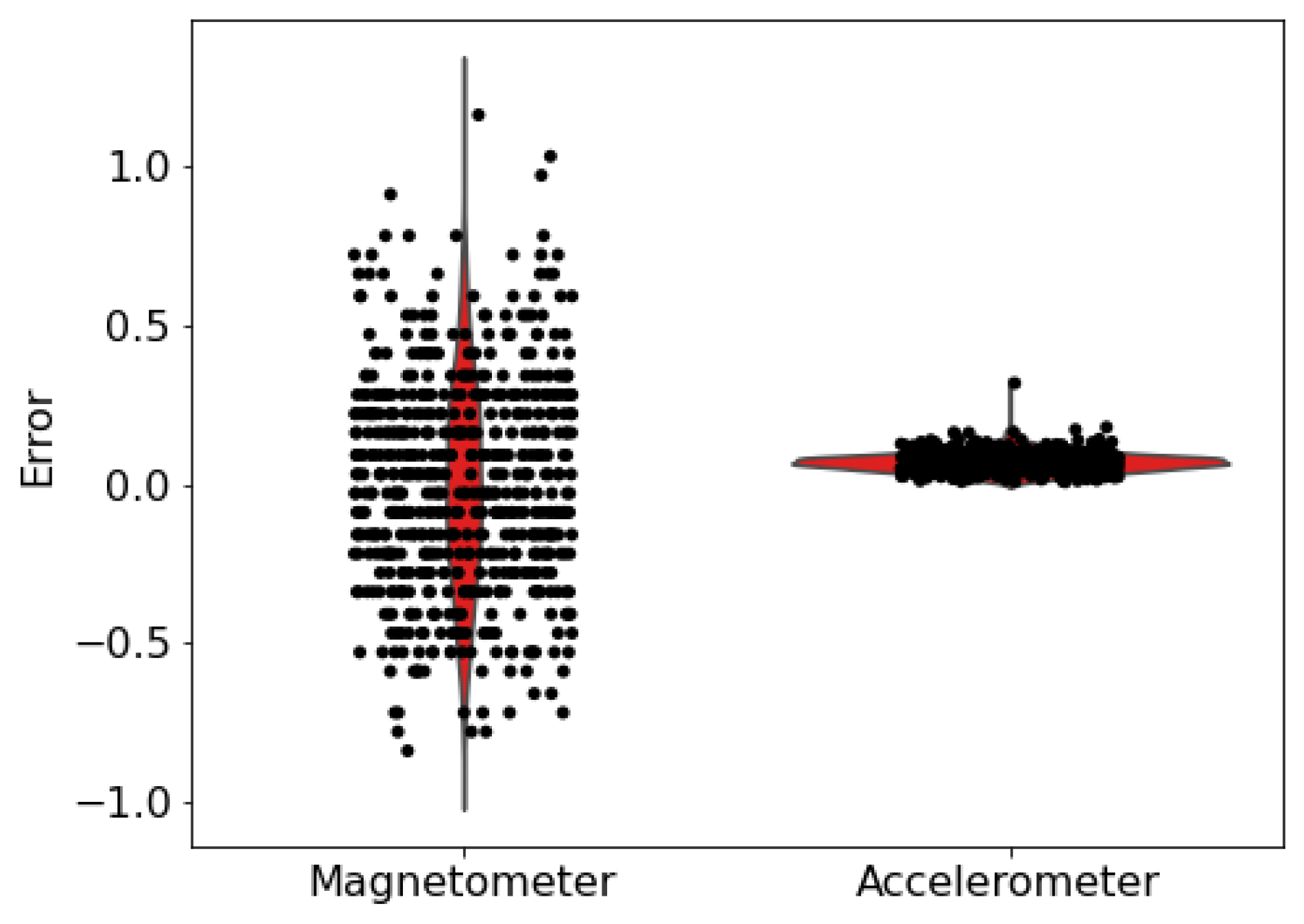
Analyzing the values we have shown in Figure 4, the magnetometer error is comprised between ±1, while the accelerometer has to be discussed more. The data in Figure 4 show an error of around ±0.2 for each sampling. As this error is summed, it is easy to understand that for longer segments the error can be in the area of 50–100 m. However, different sensors have varying precision and accuracy, hence to perform a more complete evaluation of our system we analyze different values of noises, both for angles and for lengths.
In particular, we evaluate paths of different lengths, and we also consider different levels of noise both for the accelerometer and the magnetometer. In practice, we evaluate up to = 10 and = 40. Though these values are considerably higher to what we have just shown, they also enable us to understand the possibility to be identified even with more noisy sensors. Clearly in case of excessively high noise, it may not be possible to correctly identify the original path, which may be wrongly detected. In this case, also the choice of appropriate and plays a key role.
5.2. Numerical Results
In this section we provide the performance evaluation of our proposal for a large scale study on multiple cities in the world. We are interested in understanding how such a system can be effectively used in practice, and if the city dynamics plays a role in the possibility to recognize paths performed by users. As we have already shown in Figure 2, cities differ a lot concerning urban dynamics, and we can also group them into continents which have developed specific road architectures.
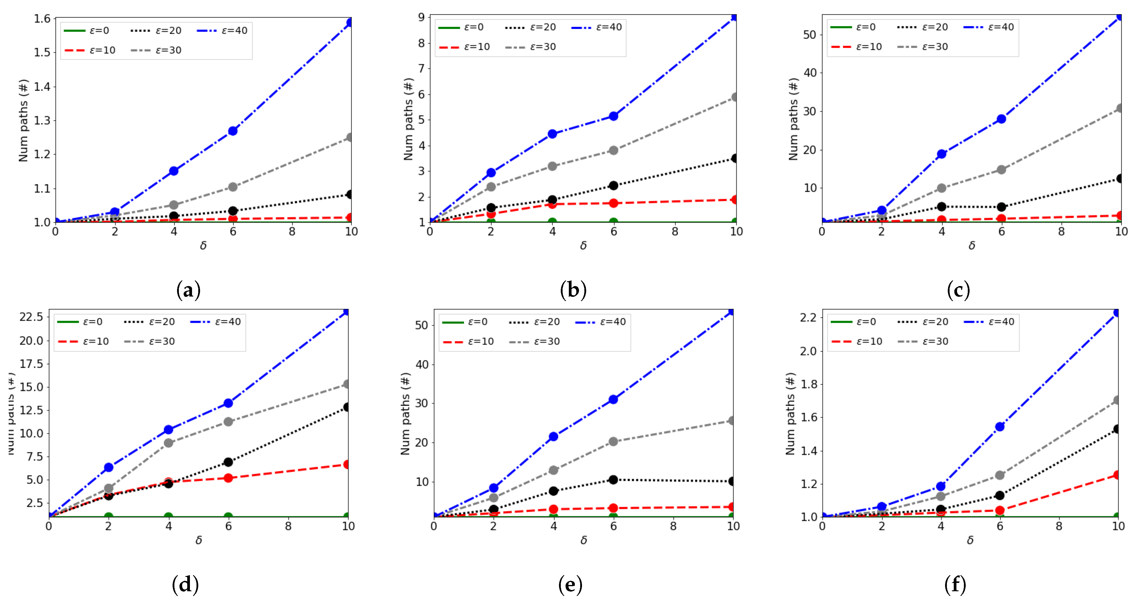
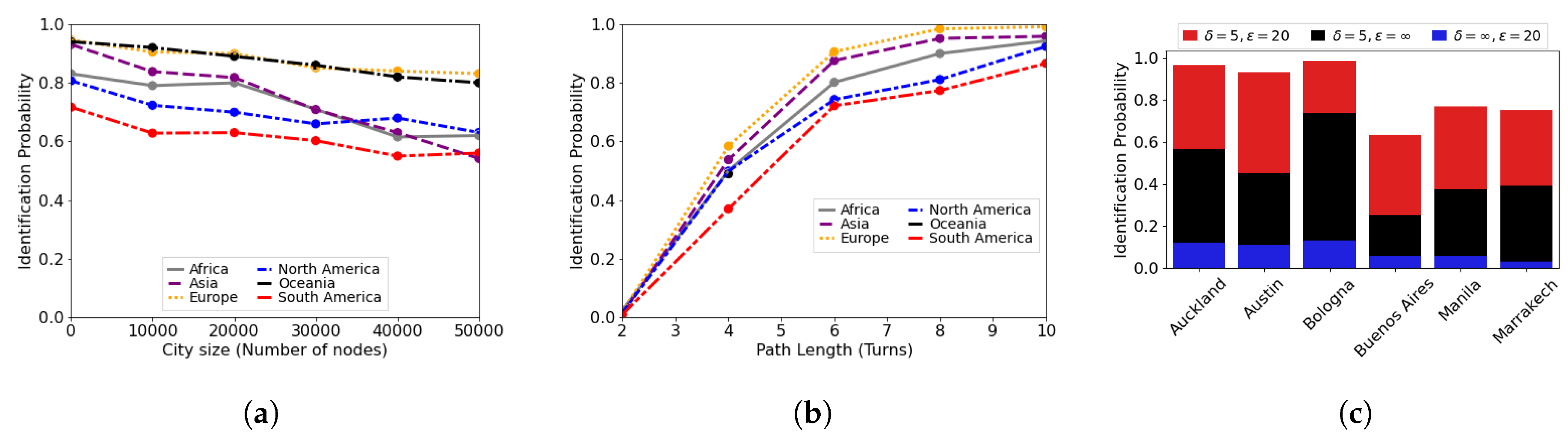
At first, we show the data about the cities we have used in our experiments, which are given in Figure 5. For our tests we evaluated six different cities, one for each continent. In this case, we show the comparison assuming a possible error due to the sensor inaccuracy both on the accelerometer and on the magnetometer. Clearly, as and increase, it is possible to find more paths in the same area, making harder to identify that traveled by the user. These results, though following a similar path, show that the quantitative results are much different depending on the city. All these six cities present similar sizes, with roughly 10,000 nodes for each of them.
In Figure 6a we plot the detection probability, defined as the probability of correctly identify a road segment over all those of the area of study, grouped according to the continent they are part of, versus the number of nodes of the city, which represents how big the area is. Figure 6a is obtained with , , and a path length of five road segments. In this case, we extended our analysis to over 8000 different cities worldwide, of different sizes hence with a different number of nodes. Clearly bigger cities may have more similar paths compared to small villages, as they would have more roads thus more possibility to have paths which share the same structure. Obviously in this case the detection probability decreases accordingly. We show a similar trend between the different continents, though Europe and Oceania are far more identifiable compared to other continents, which always have a lower identification probability.
Figure 6b shows instead the detection probability versus the length of the paths. Here we can observe that short paths are almost unidentifiable, as there are many similar in a city deployment, while longer paths are almost uniquely identifiable. For this test we selected over a hundred of cities among different continents of similar size, comprised between 8000 and 12,000 nodes. Again, we observe a similar trend regardless of the continents though with slightly different quantitative results. In particular, Europe and Oceania achieve almost perfect identification with a path eight segments long, while Africa and Asia need 10, and South and North America need two more than that. This follows the result we just presented in Figure 6a, also showing that the longer the path, the easier it is to be recognized.
Finally, Figure 6c shows the comparison concerning the identification probability when considering only data obtained through the accelerometer, only through the magnetometer, or both. Having access only to the accelerometer does not give any information about the orientation of the road segments, while having access only to data obtained through the magnetometer gives the orientation of the road segments, but not the traveled length. What can be seen is that only the accelerometer is not enough to achieve high detection accuracies, simply because there may be many roads which share the same length. The magnetometer, pictured in black, provides way more information, showing that the road angles are more characteristic compared to road lengths for discovering traveled routes. Clearly, having access to both information provides the highest detection probability, which in Figure 6c is shown in red. This analysis shows that indeed the magnetometer is far more useful in identifying paths in a city deployment, though adding data from the accelerometer raises the detection probability considerably.
5.3. CERT Performance
In this section we analyze the performance of CERT in terms of runtime and space occupancy. All tests are performed on a Dual-CPU AMD Athlon II X4 620 server, equipped with 16 GB of RAM.
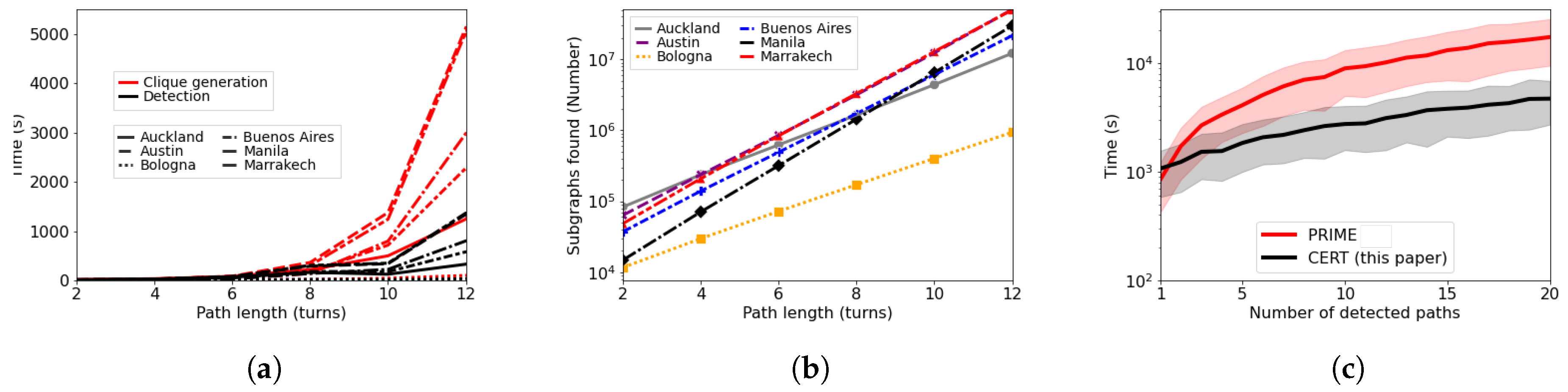
Figure 7a shows the time needed to complete the two main steps needed by CERT, the clique generation and the detection, pictured in red and black, respectively. What it is evident is that the clique generation is always greater than the simple detection of a path on the clique. It can be seen that in our test the clique generation takes roughly five times the time needed for detection. Clearly, different cities need different times to be analyzed according to their size and the city dynamics. The reason about this behavior is clarified in Figure 7b, where we show for the same cities the total number of subgraphs found by the clique detection step for several path lengths. The city of Bologna, which was the one needing the least time in Figure 7a, is also the one which has the lowest number of subgraphs found by the clique generation step, while other cities have a higher number of subgraphs eventually resulting in a longer time needed for both the clique generation and detection step.
Finally, Figure 7c shows a comparison between PRIME, which is the algorithm presented in [30] and CERT. When a single path detection is needed, PRIME performs almost identically as CERT, but as the number of detection increases, PRIME needs way more time than CERT, as we leverage on the same set of subgraphs hence reducing the detection time of the newly collected journeys.
6. Conclusions
In this work, we have shown a novel method to reconstruct driving paths in a city using only inertial sensors. The reconstruction is performed offline, leveraging dead reckoning systems to obtain the road traveled by the users, and open data to reduce the detection error by matching computed data and real data obtained from OpenStreetMap.
The focus of our analysis is to show that though generally this task is considered computationally expensive, it is possible to perform the expensive tasks in advance, making the path detection much faster.
Our results show that with as little as 10 turns it is possible to achieve almost a perfect detection of the path traveled by the user, even in big cities with several roads. A difference arises between different continents, as they have a diverse urban landscape. In fact, paths in American countries are far less identifiable compared for instance to Europe. This is due to the fact that in Europe roads are more diverse both in lengths and in orientation, while for instance in the U.S. they follow a Manhattan Grid deployment.
We have finally shown how data from the magnetometer help more in identifying the paths traveled, though the accelerometer raises the performance of the system by adding information about the road segment lengths. This also reflects the fact that for this kind of detection, recognizing turns is more beneficial than recognizing the length of the road.
As a final remark, we point out that adopting our approach can raise privacy issues, because the position of users can be retrieved without the use of GPS and without asking users the permission to use the needed sensors of the devices. In particular, systems like the one we presented in this work may undercover private information about people. Analyzing paths traveled by the same user, it is possible to rank visited places, and reveal religious beliefs, political orientation, or in general locations the user wants to remain private. To tackle this problem, one possible direction is to explicitly ask for permissions when using such sensors, as this would limit the possibility a malicious app gathers data to infer the social activities of the users.
As future works on this topic, we plan to test our algorithm with real data collected with different cars and in different cities. Clearly dealing with real data may bring more noise, hence more challenging path identification.
Author Contributions
Conceptualization, L.B.; data curation, L.B.; formal analysis, L.B.; investigation, G.C.; methodology, L.B.; supervision, G.C.; writing—original draft, L.B. and G.C.; writing—review & editing, L.B. and G.C. Both authors have read and agreed to the published version of the manuscript.
Funding
This research received no external funding.
Conflicts of Interest
The authors declare no conflict of interest.
References
- Abd Rabbou, M.; El-Rabbany, A. Tightly coupled integration of GPS precise point positioning and MEMS-based inertial systems. GPS Solut. 2015, 19, 601–609. [Google Scholar] [CrossRef]
- Narain, S.; Vo-Huu, T.D.; Block, K.; Noubir, G. The Perils of User Tracking Using Zero-Permission Mobile Apps. IEEE Secur. Priv. 2017, 15, 32–41. [Google Scholar] [CrossRef]
- Mosenia, A.; Dai, X.; Mittal, P.; Jha, N.K. PinMe: Tracking a Smartphone User around the World. IEEE Trans. Multi-Scale Comput. Syst. 2018, 4, 420–435. [Google Scholar] [CrossRef] [Green Version]
- Narain, S.; Vo-Huu, T.D.; Block, K.; Noubir, G. Inferring User Routes and Locations Using Zero-Permission Mobile Sensors. In Proceedings of the 2016 IEEE Symposium on Security and Privacy (SP), San Jose, CA, USA, 22–26 May 2016; pp. 397–413. [Google Scholar]
- Christidis, P. EU Travel Survey on Demand for Innovative Transport Systems. Available online: https://data.europa.eu/euodp/data/dataset/jrc-tem-eu_travel_survey_2014_new_technologies (accessed on 11 November 2020).
- Federal Highway Administration (FHWA). National Household Travel Survey. Available online: https://nhts.ornl.gov/ (accessed on 11 November 2020).
- German DLR. Mobility in Germany 2008. Available online: http://daten.clearingstelle-verkehr.de/223/ (accessed on 11 November 2020).
- UK Department of Transport (DfT). UK Natinoal Travel Survey 2016; Technical Report; UK Department of Transport: London, UK, 2016. Available online: https://www.gov.uk/government/collections/national-travel-survey-statistics (accessed on 11 November 2020).
- Golle, P.; Partridge, K. On the Anonymity of Home/Work Location Pairs. In Pervasive Computing; Tokuda, H., Beigl, M., Friday, A., Brush, A.J.B., Tobe, Y., Eds.; Springer: Berlin/Heidelberg, Germany, 2009; pp. 390–397. [Google Scholar]
- Dey, A.K. Understanding and Using Context. Pers. Ubiquitous Comput. 2001, 5, 4–7. [Google Scholar] [CrossRef]
- Ayu, M.A.; Mantoro, T.; Matin, A.F.A.; Basamh, S.S.O. Recognizing user activity based on accelerometer data from a mobile phone. In Proceedings of the 2011 IEEE Symposium on Computers Informatics, Kuala Lumpur, Malaysia, 20–22 March 2011; pp. 617–621. [Google Scholar]
- Bedogni, L.; Di Felice, M.; Bononi, L. Context-aware Android applications through transportation mode detection techniques. Wirel. Commun. Mob. Comput. 2016, 16, 2523–2541. [Google Scholar] [CrossRef] [Green Version]
- Casale, P.; Pujol, O.; Radeva, P. Human activity recognition from accelerometer data using a wearable device. Pattern Recognit. Image Anal. 2011, 6669 LNCS, 289–296. [Google Scholar]
- Reddy, S.; Mun, M.; Burke, J.; Estrin, D.; Hansen, M.; Srivastava, M. Using mobile phones to determine transportation modes. ACM Trans. Sens. Netw. 2010, 6, 1–27. [Google Scholar] [CrossRef]
- Chen, L.; Yang, D.; Nogueira, M.; Wang, C.; Zhang, D. Data-Driven C-RAN Optimization Exploiting Traffic and Mobility Dynamics of Mobile Users. Available online: https://0-ieeexplore-ieee-org.brum.beds.ac.uk/document/8981890 (accessed on 17 November 2020).
- Leppäkoski, H.; Collin, J.; Takala, J. Pedestrian Navigation Based on Inertial Sensors, Indoor Map, and WLAN Signals. J. Signal Process. Syst. 2013, 71, 287–296. [Google Scholar] [CrossRef]
- Cankaya, I.A.; Koyun, A.; Yigit, T.; Yuksel, A.S. Mobile indoor navigation system in iOS platform using augmented reality. In 2015 9th International Conference on Application of Information and Communication Technologies (AICT); IEEE: New York, NY, USA, 2015; pp. 281–284. [Google Scholar] [CrossRef]
- Rehman, U.; Cao, S. Augmented-Reality-Based Indoor Navigation: A Comparative Analysis of Handheld Devices Versus Google Glass. IEEE Trans. Hum.-Mach. Syst. 2016, 47, 140–151. [Google Scholar] [CrossRef]
- Bedogni, L.; Franzoso, F.; Bononi, L. A Self-Adapting Algorithm Based on Atmospheric Pressure to Localize Indoor Devices. In Proceedings of the 2016 IEEE Global Communications Conference (GLOBECOM), Washington, DC, USA, 4–8 December 2016; pp. 1–6. [Google Scholar] [CrossRef]
- Jimenez, A.; Seco, F.; Prieto, C.; Guevara, J. A comparison of Pedestrian Dead-Reckoning algorithms using a low-cost MEMS IMU. In 2009 IEEE International Symposium on Intelligent Signal Processing; IEEE: New York, NY, USA, 2009; pp. 37–42. [Google Scholar] [CrossRef]
- Kang, W.; Han, Y. SmartPDR: Smartphone-Based Pedestrian Dead Reckoning for Indoor Localization. IEEE Sens. J. 2015, 15, 2906–2916. [Google Scholar] [CrossRef]
- Wahab, A.A.; Khattab, A.; Fahmy, Y.A. Two-way TOA with limited dead reckoning for GPS-free vehicle localization using single RSU. In 2013 13th International Conference on ITS Telecommunications (ITST); IEEE: New York, NY, USA, 2013; pp. 244–249. [Google Scholar] [CrossRef]
- Han, J.; Owusu, E.; Nguyen, L.T.; Perrig, A.; Zhang, J. ACComplice: Location inference using accelerometers on smartphones. In Proceedings of the 2012 Fourth International Conference on Communication Systems and Networks (COMSNETS 2012), Bangalore, India, 3–7 January 2012; pp. 1–9. [Google Scholar]
- Chang, Q.; Van de Velde, S.; Wang, W.; Li, Q.; Hou, H.; Heidi, S. Wi-Fi Fingerprint Positioning Updated by Pedestrian Dead Reckoning for Mobile Phone Indoor Localization. In China Satellite Navigation Conference (CSNC) 2015 Proceedings: Volume III; Sun, J., Liu, J., Fan, S., Lu, X., Eds.; Springer: Berlin/Heidelberg, Germany, 2015; pp. 729–739. [Google Scholar]
- Zhang, X.; Jin, Y.; Tan, H.X.; Soh, W.S. CIMLoc: A crowdsourcing indoor digital map construction system for localization. In 2014 IEEE Ninth International Conference on Intelligent Sensors, Sensor Networks and Information Processing (ISSNIP); IEEE: New York, NY, USA, 2014; pp. 1–6. [Google Scholar] [CrossRef] [Green Version]
- Aguilar Herrera, J.C.; Hinkenjann, A.; Ploger, P.G.; Maiero, J. Robust indoor localization using optimal fusion filter for sensors and map layout information. In International Conference on Indoor Positioning and Indoor Navigation; IEEE: New York, NY, USA, 2013; pp. 1–8. [Google Scholar] [CrossRef]
- Link, J.A.B.; Smith, P.; Viol, N.; Wehrle, K. FootPath: Accurate map-based indoor navigation using smartphones. In 2011 International Conference on Indoor Positioning and Indoor Navigation; IEEE: New York, NY, USA, 2011; pp. 1–8. [Google Scholar] [CrossRef] [Green Version]
- Bedogni, L.; Gramaglia, M.; Vesco, A.; Fiore, M.; Härri, J.; Ferrero, F. The Bologna ringway dataset: Improving road network conversion in SUMO and validating urban mobility via navigation services. IEEE Trans. Veh. Technol. 2015, 64, 5464–5476. [Google Scholar] [CrossRef] [Green Version]
- Luxen, D.; Vetter, C. Real-time routing with OpenStreetMap data. In Proceedings of the 19th ACM SIGSPATIAL International Conference on Advances in Geographic Information Systems—GIS ’11, Chicago, IL, USA, 1–4 November 2011; p. 513. [Google Scholar] [CrossRef]
- Bedogni, L.; Bononi, L. Vehicular Route Identification Using Mobile Devices Integrated Sensors. In Proceedings of the 2019 IEEE International Conference on Pervasive Computing and Communications Workshops (PerCom Workshops), Kyoto, Japan, 11–15 March 2019; pp. 820–825. [Google Scholar] [CrossRef]
- Fiedler, M.; Markham, T.L. An inequality for the Hadamard product of an M-matrix and an inverse M-matrix. Linear Algebra Appl. 1988, 101, 1–8. [Google Scholar] [CrossRef] [Green Version]
Figure 1.
Example run of the CERT algorithm. (a) shows G(P), (b) shows instead G(I). The clique generation, pictured in (c) finds all the subgraphs of of length N = 4 according to the length of G(P). The detection step is shown in (d), where we find the best possible match of G(P).
Figure 1.
Example run of the CERT algorithm. (a) shows G(P), (b) shows instead G(I). The clique generation, pictured in (c) finds all the subgraphs of of length N = 4 according to the length of G(P). The detection step is shown in (d), where we find the best possible match of G(P).

Figure 2.
(a,b) show the PDF of the road angles and road lengths for different worldwide cities, respectively. (c) shows the α and β values for different sized cities in the EU and US.
Figure 2.
(a,b) show the PDF of the road angles and road lengths for different worldwide cities, respectively. (c) shows the α and β values for different sized cities in the EU and US.

Figure 3.
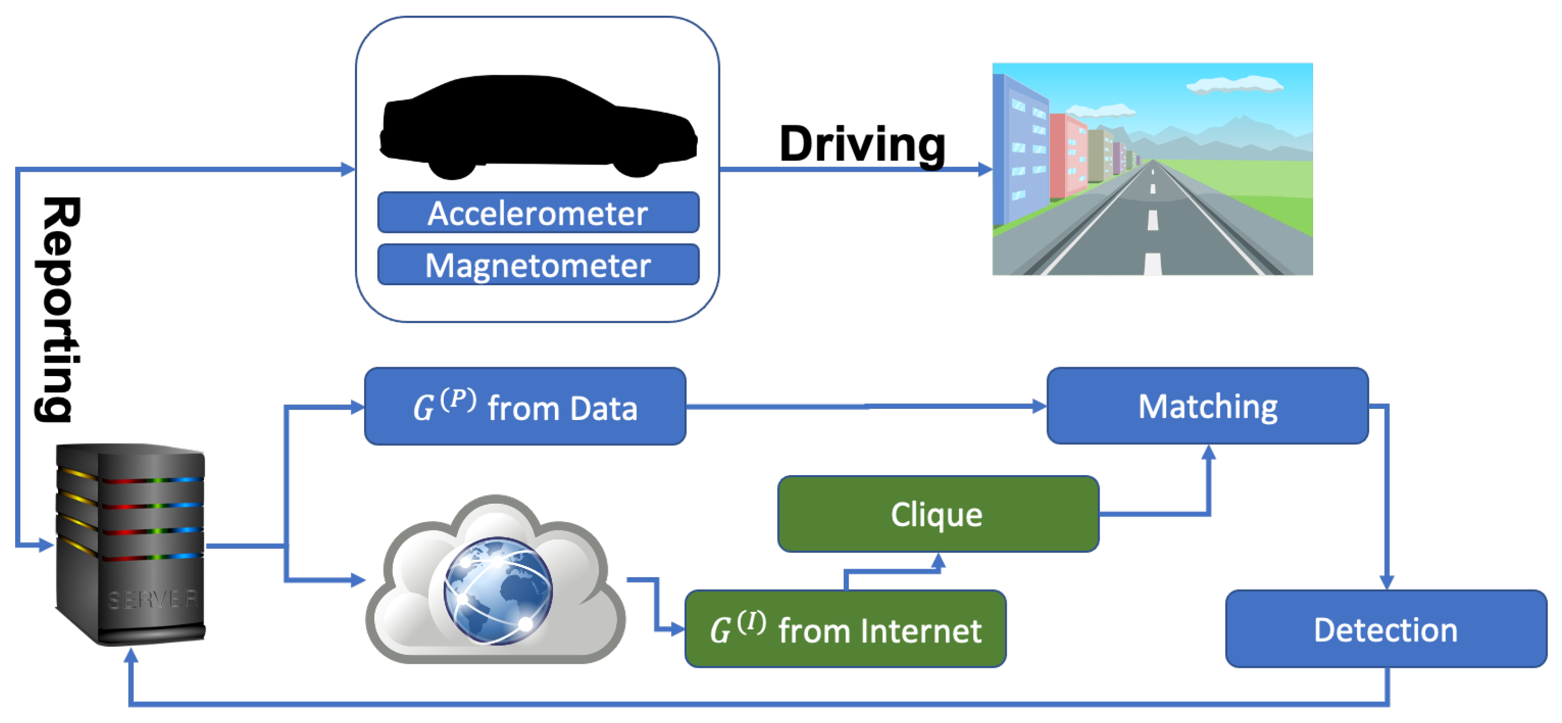
Overarching schema of our proposal. Sensors read data from the car movement, which are reported to a central server. Here we create the two graphs, and , and from the latter we find all the possible subgraphs of any size. We then perform the matching between and the subgraphs we found, eventually detecting the best possible match and reporting it back. We note that the download and the clique operation can be performed in advance, and stored in memory, to save time for the matching operation.
Figure 3.
Overarching schema of our proposal. Sensors read data from the car movement, which are reported to a central server. Here we create the two graphs, and , and from the latter we find all the possible subgraphs of any size. We then perform the matching between and the subgraphs we found, eventually detecting the best possible match and reporting it back. We note that the download and the clique operation can be performed in advance, and stored in memory, to save time for the matching operation.

Figure 4.
Measurement distribution gathered with 10 different smartphones placed at a constant direction.
Figure 4.
Measurement distribution gathered with 10 different smartphones placed at a constant direction.

Figure 5.
Number of paths in different cities, varying ϵ and δ. The cities tested are Bologna, Italy (a), Austin, Texas (b), Marrakech, Morocco (c), Manila, Philippines (d), Buenos Aires, Argentina (e), and Auckland, New Zealand (f).
Figure 5.
Number of paths in different cities, varying ϵ and δ. The cities tested are Bologna, Italy (a), Austin, Texas (b), Marrakech, Morocco (c), Manila, Philippines (d), Buenos Aires, Argentina (e), and Auckland, New Zealand (f).

Figure 6.
(a) shows the Identification probability for increasingly large cities. (b) shows the same metric, plotted instead against the path length. Finally (c) shows the comparison when considering only the accelerometer, only the magnetometer, or both.
Figure 6.
(a) shows the Identification probability for increasingly large cities. (b) shows the same metric, plotted instead against the path length. Finally (c) shows the comparison when considering only the accelerometer, only the magnetometer, or both.

Figure 7.
(a) shows the time needed to perform the clique generation and the detection for different cities worldwide. (b) shows the number of different subgraphs found for the same cities, versus the length of the path. Finally (c) shows the comparison in time between this work and [30].
Figure 7.
(a) shows the time needed to perform the clique generation and the detection for different cities worldwide. (b) shows the number of different subgraphs found for the same cities, versus the length of the path. Finally (c) shows the comparison in time between this work and [30].


Table 1.
Related work classification.
| Reference | Type | Data |
|---|---|---|
| [19] | Indoor navigation | Barometer |
| [20] | Indoor navigation | Barometer |
| [26] | Indoor navigation | Sensor fusion |
| [27] | Indoor navigation | Accelerometer and Open data |
| [22] | Indoor navigation | Accelerometer |
| [21] | GPS correction | Accelerometer |
| [28] | Vehicular traces improvement | Open data |
| [29] | Map Enhancement | Open data |
| [25] | Map Enhancement | Accelerometer, Magnetometer and Gyroscope |
| [24] | Pedestrian tracking | Wi-Fi and Open data |
| [23] | Driving tracking | Accelerometer |
| [2] | Driving tracking | Accelerometer, Magnetometer and Gyroscope |
| [30] | Driving tracking | Accelerometer, Magnetometer and Gyroscope |
Publisher’s Note: MDPI stays neutral with regard to jurisdictional claims in published maps and institutional affiliations. |
© 2020 by the authors. Licensee MDPI, Basel, Switzerland. This article is an open access article distributed under the terms and conditions of the Creative Commons Attribution (CC BY) license (http://creativecommons.org/licenses/by/4.0/).
Share and Cite
MDPI and ACS Style
Bedogni, L.; Cabri, G. Identification of Social Aspects by Means of Inertial Sensor Data. Information 2020, 11, 534. https://0-doi-org.brum.beds.ac.uk/10.3390/info11110534
AMA Style
Bedogni L, Cabri G. Identification of Social Aspects by Means of Inertial Sensor Data. Information. 2020; 11(11):534. https://0-doi-org.brum.beds.ac.uk/10.3390/info11110534
Chicago/Turabian StyleBedogni, Luca, and Giacomo Cabri. 2020. "Identification of Social Aspects by Means of Inertial Sensor Data" Information 11, no. 11: 534. https://0-doi-org.brum.beds.ac.uk/10.3390/info11110534
Note that from the first issue of 2016, this journal uses article numbers instead of page numbers. See further details here.