
A Markov Chain Monte Carlo Algorithm for Spatial Segmentation


Department of Mathematics and Statistics, Macquarie University, Sydney, NSW 2109, Australia
*
Author to whom correspondence should be addressed.
Information 2021, 12(2), 58; https://0-doi-org.brum.beds.ac.uk/10.3390/info12020058
Submission received: 30 December 2020
/
Revised: 25 January 2021
/
Accepted: 27 January 2021
/
Published: 30 January 2021
(This article belongs to the Special Issue Data Modeling and Predictive Analytics)
Abstract
:Spatial data are very often heterogeneous, which indicates that there may not be a unique simple statistical model describing the data. To overcome this issue, the data can be segmented into a number of homogeneous regions (or domains). Identifying these domains is one of the important problems in spatial data analysis. Spatial segmentation is used in many different fields including epidemiology, criminology, ecology, and economics. To solve this clustering problem, we propose to use the change-point methodology. In this paper, we develop a new spatial segmentation algorithm within the framework of the generalized Gibbs sampler. We estimate the average surface profile of binary spatial data observed over a two-dimensional regular lattice. We illustrate the performance of the proposed algorithm with examples using artificially generated and real data sets.
1. Introduction
Identifying homogeneous domains is one of the important problems in spatial data analysis since spatial data are very often heterogeneous. For example, survey data may be collected from a number of regions or areas that have different socioeconomic indicator variables. To overcome the problem that there may not be a unique statistical model effectively describing the spatial data, we can divide the data into a number of homogeneous regions (or domains). The spatial segmentation, which is also known as partitioning or clustering, would allow us to develop and fit different appropriate statistical models for each domain. The spatial clustering consists of two problems: identifying the boundaries of the domains and their number.
There is an extensive literature on a variety of different clustering algorithms. These include hierarchical methods (for example, bottom-up or agglomerative and top-down or divisive algorithms) and optimization methods (for example, the k-means algorithm) [1]. Clustering algorithms are widely used in many different areas, including spatial epidemiology, signal processing, ecological and economic applications; see [2]. Even though there are various algorithms for different types of clustering problems, there are no global algorithms to solve them effectively. In this paper, we are particularly interested in developing an effective Markov chain Monte Carlo (MCMC) algorithm for a spatial segmentation problem. Recently Bayesian approaches have become quite popular for such problems, and many Bayesian algorithms have been proposed in many different contexts. In particular, one of the important problems in epidemiology is to classify regions depending on their level of a disease risk. A spatial clustering approach with the Bayesian framework is discussed in [3]. In [4], the authors present a Bayesian approach to estimate the spatial pattern in disease risk and to identify regions with have high/low disease risks.
Ecological applications is one of the areas where spatial segmentation plays a very important role. In case of analysing large spatial data sets, it is quite common that the spatial distribution of plants (or animals) is heterogeneous. In [5], the authors consider a class of Bayesian statistical models in order to identify changes and their locations in ecological data. In [6], the authors apply a change-point detection methodology to detect plant patches. An algorithm based on a binary segmentation method within the change-point detection framework in order to identify homogeneous domains has recently been developed in [7]. Climate change studies is another area that commonly uses spatial segmentation methods. In [8], the authors consider a non-parametric test within a Bayesian change-point detection framework and a hidden Markov model to find changes in the rainfall and temperature patterns over India. In image recognition, spatial segmentation methods are used to identify boundaries of an image. For example, an MCMC method to identify closed object boundaries in gray-scale images is proposed in [9]. In [10], the author proposes a wavelet method to estimate jumps and sharp curves of a function in the plane.
There are many applications of spatial segmentation in finance and economics. For instance, a novel hybrid clustering algorithm and a pattern recognition scheme are presented in [11] for time series forecasting. In [12], the authors proposed a class of spatial econometric methods in spatial clustering of industries in the space. Recently, an economic decision support system based on fuzzy C-mean clustering is proposed in [13] for economic forecasting. A hybrid algorithm is presented in [14] for spatial small area estimation to use in agricultural and resource economics surveys. A variety of clustering approaches for financial data analysis is discussed in [15].
The objective of our study, which is motivated by analysis of the distribution of plant species, is to identify homogeneous domains in binary spatial data observed over a two-dimensional regular lattice. This model belongs to the class of autologistic models introduced by Besag [16]. Parameter estimation or drawing samples from posterior distribution for this model is a notoriously difficult problem due to the complex form of likelihood function.The alternative methods to maximum likelihood estimate include pseudolikelihood and Monte Carlo maximum likelihood estimators [17,18]. To analyse this model within the Bayesian framework, a significant step was made by Moller [19], who proposed an auxiliary variable MCMC method that draws independent samples from unnormalised density by constructing the proposal distribution that cancels the normalising constant from Metropolis-Hastings ratio. This method works well for autologistic model but it is very slow and, as a result, this theoretically sound Bayesian inference is impractical for large lattices because the perfect sampler is of order . Faster approximate Bayesian approaches exist but lack theoretical justification [20]. Recently, a double Metropolis-Hastings sampler for autologistic model for spatial data is proposed in [21]. Unlike other auxiliary variables algorithms, this sampler removes the need for exact sampling, the auxiliary variable being generated using Metropolis-Hastings kernels and it produces the same accurate results as other MCMC algorithms, but using much less CPU time.
Our study aims to develop effective procedures based on an MCMC algorithm within the generalized Gibbs sampler (GGS) framework for estimating the average surface profile explaining the heterogeneity of the data. The GGS is originally proposed in [22] and it is particularly useful for sampling from distributions defined on spaces in which the dimension varies from point to point or in which points are not easily defined in terms of coordinates. We consider our problem as a change-point detection problem, which is commonly used in analysing time series to detect abrubt points and their locations. For more details on change-point problems, applications and available methods, see [23,24,25]. The GGS approach is already used in multiple change-point problem in order to segment a long DNA sequence into intervals of approximately uniform composition [22]. In this paper, we present a novel algorithm expanding the GGS from a one-dimensional change-point problem to a two-dimensional segmentation problem. For more details on the GGS and its theoritical properties, see [22].
This paper is organized as follows. In Section 2, we formulate the spatial segmentation problem. In Section 3, we introduce the main concepts of the GGS, while Section 4 presents a new spatial segmentation algorithm within the GGS framework. In Section 5, we illustrate the proposed algorithm’s performance with three examples using artificially generated and real data sets. Finally, Section 6 provides a discussion of the results and concluding remarks.
2. The Spatial Segmentation Problem
Let us formally introduce the spatial segmentation problem. We are given spatial binary data, a lattice with zeros and ones (presence-absence data), which can be represented by an matrix, B. A segmentation of B is specified by giving the number of cuts N (horizontal and vertical) and the domains with their boundaries parallel to the sides of the lattice. The position of each domain , , can be defined by the four edges , left, right, up and down, respectively. A maximum number of cuts is specified, where . The model for the data assumes that within each domain observations are generated by independent Bernoulli trials with probability of success (presence of the plant indicates “1”) that depends on the domain. Thus, the joint probability density function (pdf) of spatial data B conditional on N, , and , is given by
where is the number of ones in domain and is the number of zeros in that same domain.
To use the Bayesian framework, a prior distribution must be defined on the set of possible values of , denoted
with
where , , , or means that the boundary of the n-th domain coincides with the edge of the lattice.
We assume discrete uniform priors both on the number of domains and on their positions on the sets and , respectively. Alternatively, a truncated Poisson distribution may be taken as a prior distribution on the number of domains. A continuous uniform prior is assumed on for each . This means that the overall prior is a constant. Therefore, taking into account (1), the posterior density function at point , having observed spatial data B, is given by
3. The Generalized Gibbs Sampler
The generalized Gibbs sampler is a Markov chain Monte Carlo technique that is particularly useful for sampling from distributions defined on spaces in which the dimension varies from point to point or in which points are not easily defined in terms of coordinates. A number of MCMC samplers are available for the purpose of Bayesian model determination and comparison. These samplers allow transisitons between different models and are important where there is uncertainty about not only the parameters of a model, but also about the model itself. These samplers are referred as model-switching samplers and can be used for Bayesian model selection, model evaluation, model averaging and hypothesis testing. An example of this type of sampler is the Reversible-jump MCMC sampler, which is a generalization of the Metropolis-Hastings algorithm. In this paper, we use the GGS, a model-switching sampler that generalizes the Gibbs sampler, provides an alternative that is easy to implement and often highly efficient [22,26]. However, no systematic comparison of the advantages and disadvantages of the GGS versus the Reversible-jump sampler has been performed. The dimension in this algorithm does not need to be fixed and it provides flexibility to sample from varying dimensional spaces and it has been applied to some very high dimensional problems [27].
Let us explain the GGS in mathematical terms. Consider a Markov chain on the set , where is the target set and is an auxiliary set. Here, we assume that both sets are finite. Let be the target pdf (for example, see (2)), defined on . Each transition of the Markov chain consists of two steps: the Q-step, followed by the R-step. In other words, the transition matrix P of the Markov chain is given by the product . The first step is , according to a transition matrix Q, which changes only the y-coordinates. , where is a transition matrix on . Let be a stationary distribution for . The second step is , according to a transition matrix R. The transition matrix R can be defined as: , for all , where is a normalisation constant. Note that is a set containing the point . The distribution
is trivially stationary with respect to Q, and satisfies detailed balance with respect to R, and hence is a stationary distribution with respect to the Markov chain. For more details, see [22,26]. The following steps illustrate the main idea of this algorithm. First start with an arbitrary , then perform the following steps iteratively:
- Q-step: Given , generate Y from
- R-step: Given Y generate from .
This algorithm generates a Markov chain such that the limiting distribution of as is , provided that P is irreducible and aperiodic.
The GGS framework makes it possible to obtain many different samplers.The Gibbs sampler, the Metropolis-Hastings sampler, the Reversible-jump sampler and the Slice sampler are special cases of the GGS. These algorithms can be used in the context of simulated annealing to determine the maximum of , attained at the “best model” x. Furthermore, GGS can be extended to the general case of infinite sets and . For more details on the GGS, see [22].
4. The GGS for the Spatial Segmentation Problem
In this section, we propose the GGS for the spatial segmentation problem described above. We consider this problem within the change-point detection framework and develop a GGS algorithm to estimate the average surface profile explaining the heterogeneity of data. Multiple change-point problems have commonly been utilized to illustrate model switching samplers [28,29]. The GGS is also previously used in change-point problem [22]. In this study, we use the GGS for the spatial segmentation problem. Here, we assume that the observations and the clusters are conditionally independent.
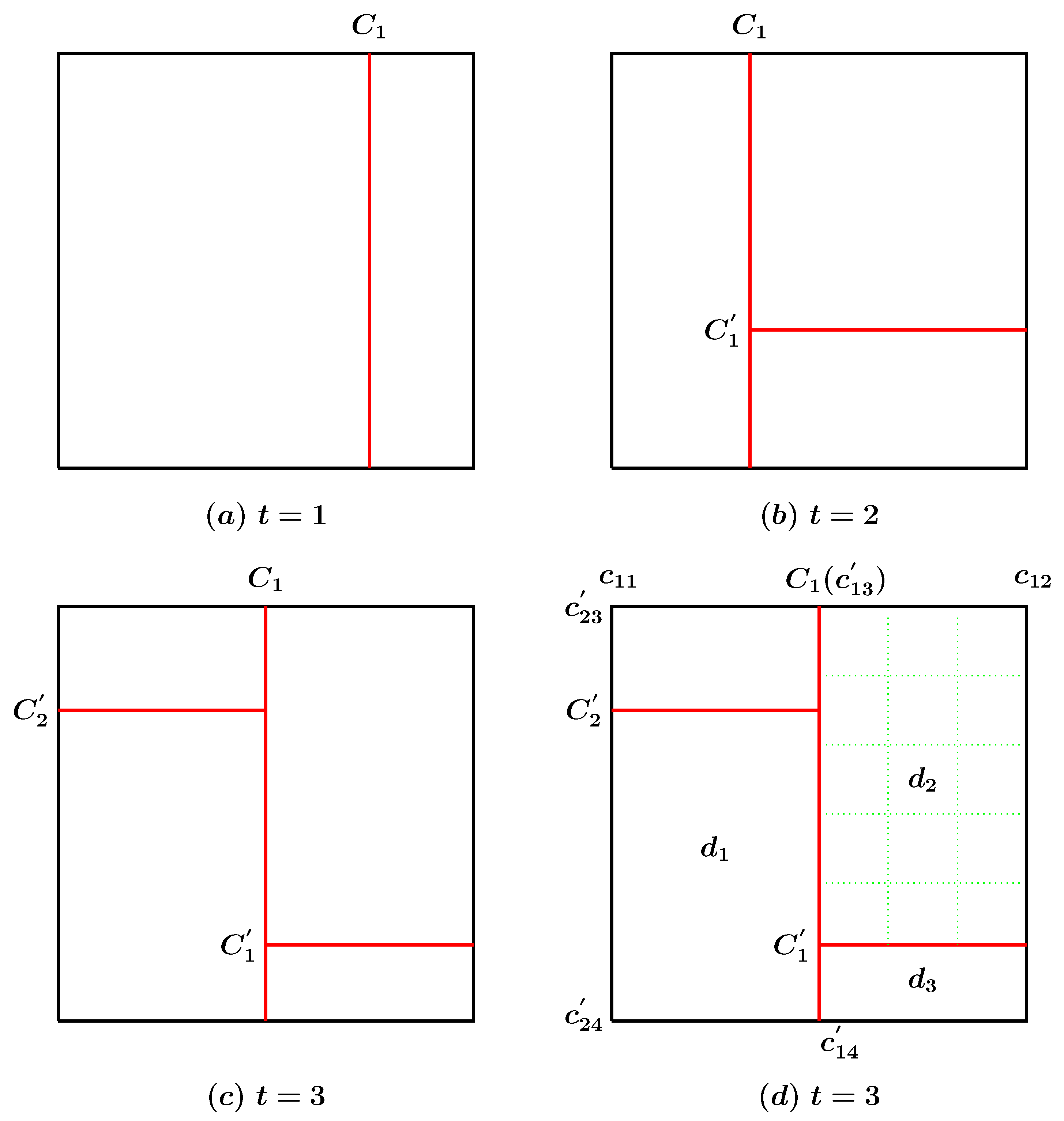
Let us number all cuts from 1 to N for a model x and consider the n-th cut, . Define , where and are, respectively, the leftmost and rightmost possible cuts to the n-th cut when the orientation of the cut is vertical; and are, respectively, the uppermost and downmost possible cuts to the n-th cut when the orientation of the cut is horizontal. Figure 1 shows the visualization of some moves.
Let be the set of possible cuts to the left (if it is a vertical) to the n-th cut or above (if it is a horizontal) the n-th cut; be the set of possible cuts to the right (if it is a vertical) to the n-th cut or below (if it is a horizontal) the n-th cut:
The GGS algorithm cycles through a sequence of steps in which parts of a sampled element are updated, while other parts are held constant. These different types of updates are analogous to the coordinate updates of the conventional Gibbs sampler and are known as “move types”. The GGS algorithm for this problem may be constructed as follows. Two broad classes of moves are allowed, labelled “Ins“ and “Del”, which illustrate insertion and deletion of a cut. This technique allows the number of cuts to vary: it cycles through domains inserting and deleting cuts, and shifting cut positions. For a model x with N cuts, there are domains into which a new cut may be inserted, and N cuts that may be deleted. Depending on the orientation of a cut, each cut has a chance to move left or right (if it is a vertical cut); up or down (if it is a horizontal cut), or stay on same position. There are thus move types for a cycle. We consider that all domains are equally likely to be chosen to add a new cut.
For the Q-step, define a transition matrix
The design of the transition matrix in the Q-step follows the idea of the original GGS algorithm (see [22] (Section 5)) expanding from one dimensional change-point problem to two dimensional segmentation problem. This preserves the properties of the GGS discussed in Section 3. In the proposed algorithm, the move type is chosen according to the stationary distribution of , which is , discrete uniform with probability function . For the R-step, we use the set of models obtained by changing only a single domain of x, either by changing the Bernoulli parameter for that domain, or by splitting it into two new domains with separate Bernoulli parameters.
Let be the set of possible cuts in domain and be the set of possible cuts that coincide with one of the edges of domain :
For the R-step, define to be the set of models obtained by changing only domain , either by changing the Bernoulli parameter for that domain, or by splitting it into two domains ( and ) with separate Bernoulli parameters. For given n and x, we define to be the set of models obtained by changing the Bernoulli parameter for domain , and to be the set of models obtained by inserting a new cut at and setting two new Bernoulli parameters for those two domains. Thus,
if x has fewer than cuts and
if x has total cuts. R-step can simply be implemented as follows.
We take the densities in the R step proportional to g, which is defined in (1). We compute the integral of g over , and integrals of g over , for each . For example, consider when B has fewer than cuts:
- Calculate the weights for and .
- Select an element with probabilities proportional to the weights calculated in Step 1.
- If is selected, update by sampling from a beta distribution with parameters and . Otherwise, if is selected, insert a new cut at and select new Bernoulli parameters for domains and by sampling from beta distributions with parameters and , respectively.
The R-step is simply a conventional Gibbs coordinate update in which a new value for is generated by sampling from a beta distribution with parameters and .
5. Numerical Results
In this section, we discuss three examples with artificially generated and real spatial data sets to illustrate the usefulness of the proposed algorithm. The first two data sets are artificial matrices with known distributions, while in the third example we use real presence-absence plant data [30].
We compare the proposed GGS algorithm to the Sequential Importance Sampling (SIS) algorithm, which is previously developed for the same type of spatial segmentation problem [31]. Both SIS and GGS algorithms aim at the same posterior distribution but they are different in their nature. The SIS algorithm finds new cuts based on the cuts obtained previously and it calculates weights with respect to proposal density and target density sequentially. The obtained profile is a weighted average of M (for example M = 100) profiles obtained by the SIS. On the other hand, the proposed GGS generates domains by adding a new cut, deleting existing cuts, or moving to new positions by aiming the target distribution.
We use the parameters of Bernoulli distribution to calculate the Root Mean Squared Error (RMSE). We consider the values for each cell of the matrix B while the estimated values for each cell within a particular domain remains the same. It is calculated as
where , are the estimated and the true values, respectively, for each cell of the matrix; are the corresponding rows and columns; and are the dimensions of the matrix.
One of the technical difficulties in MCMC methods is that samples will typically be autocorrelated within the chain. This will increase the uncertainty of estimation of the posterior quantities [32]. We need to estimate an effective sample size for each parameter, which plays an important role in the MCMC central limit theorem as the number of independent samples plays in the standard central limit theorem. In this study, we use the following formula to estimate the effective sample size of N samples generated with autocorrelations ,
We follow [33] to estimate the autocorrelations . It can be assumed that decays approximately exponentially [34]. It follows that,
where is the exponential autocorrelation time, which can be calculated in the following way:
In our study, each draw is a matrix. First, we calculate for each cell of the matrix. Second, we find the maximal autocorrelation value and use it to calculate . Then we estimate the effective sample size (4).
5.1. Artificial Data: Example 1
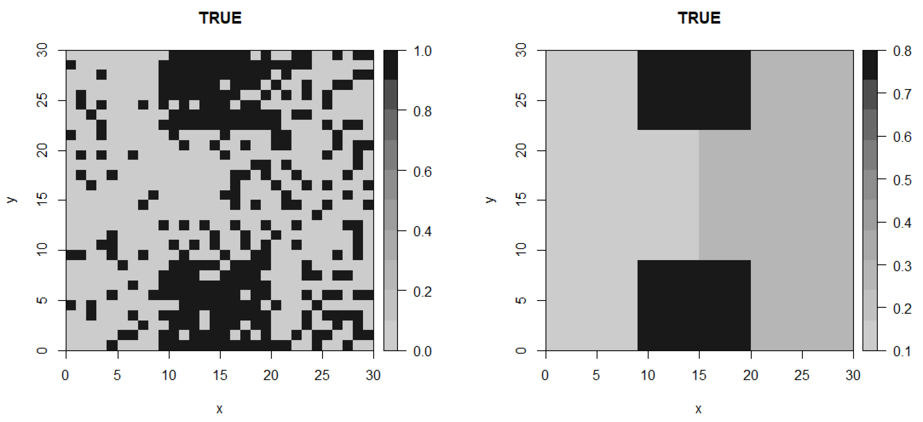
Let B be a matrix of independent Bernoulli random variables generated with the parameters given in Table 1. The true profile of this matrix can be seen in Figure 2.
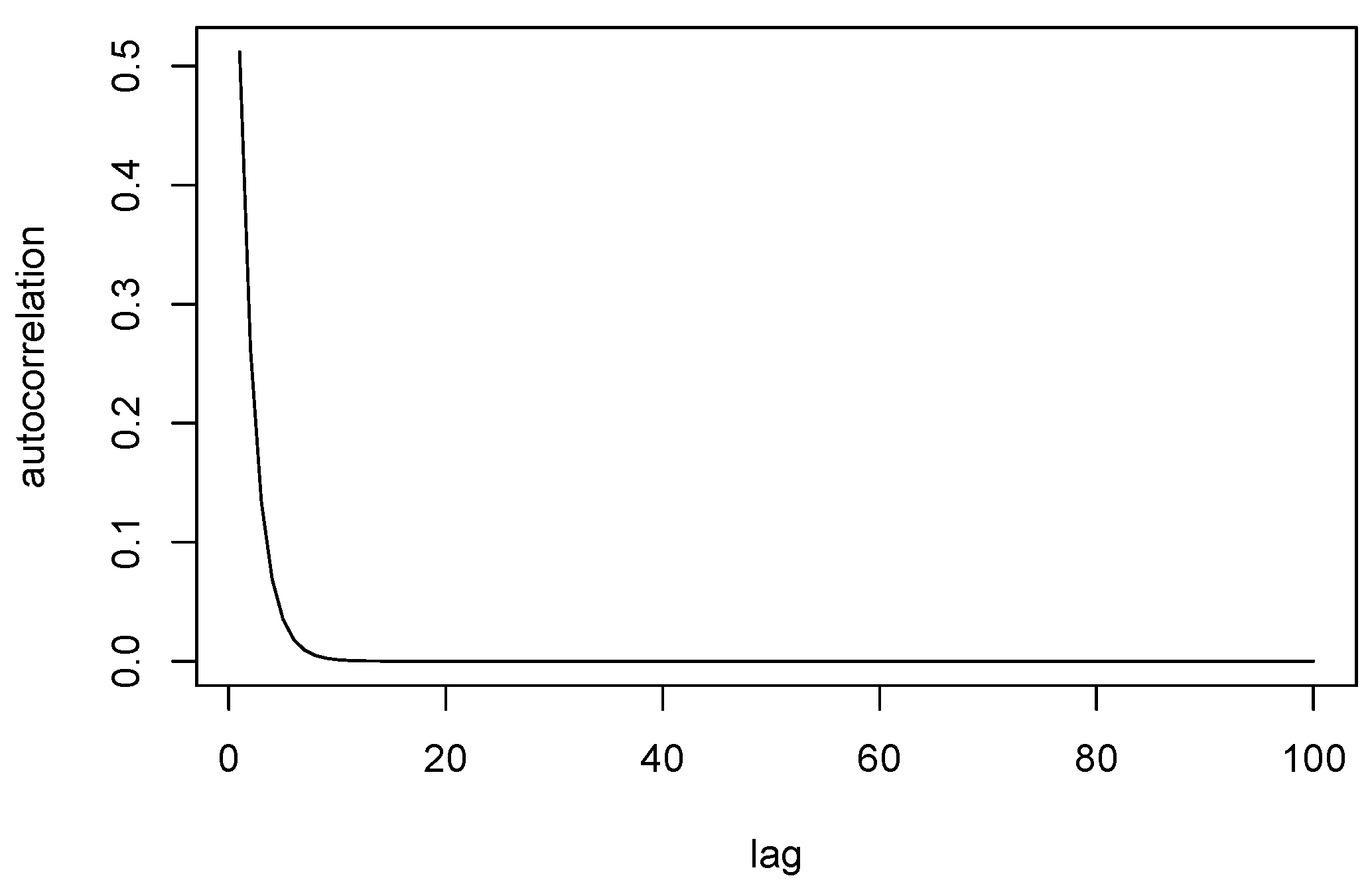
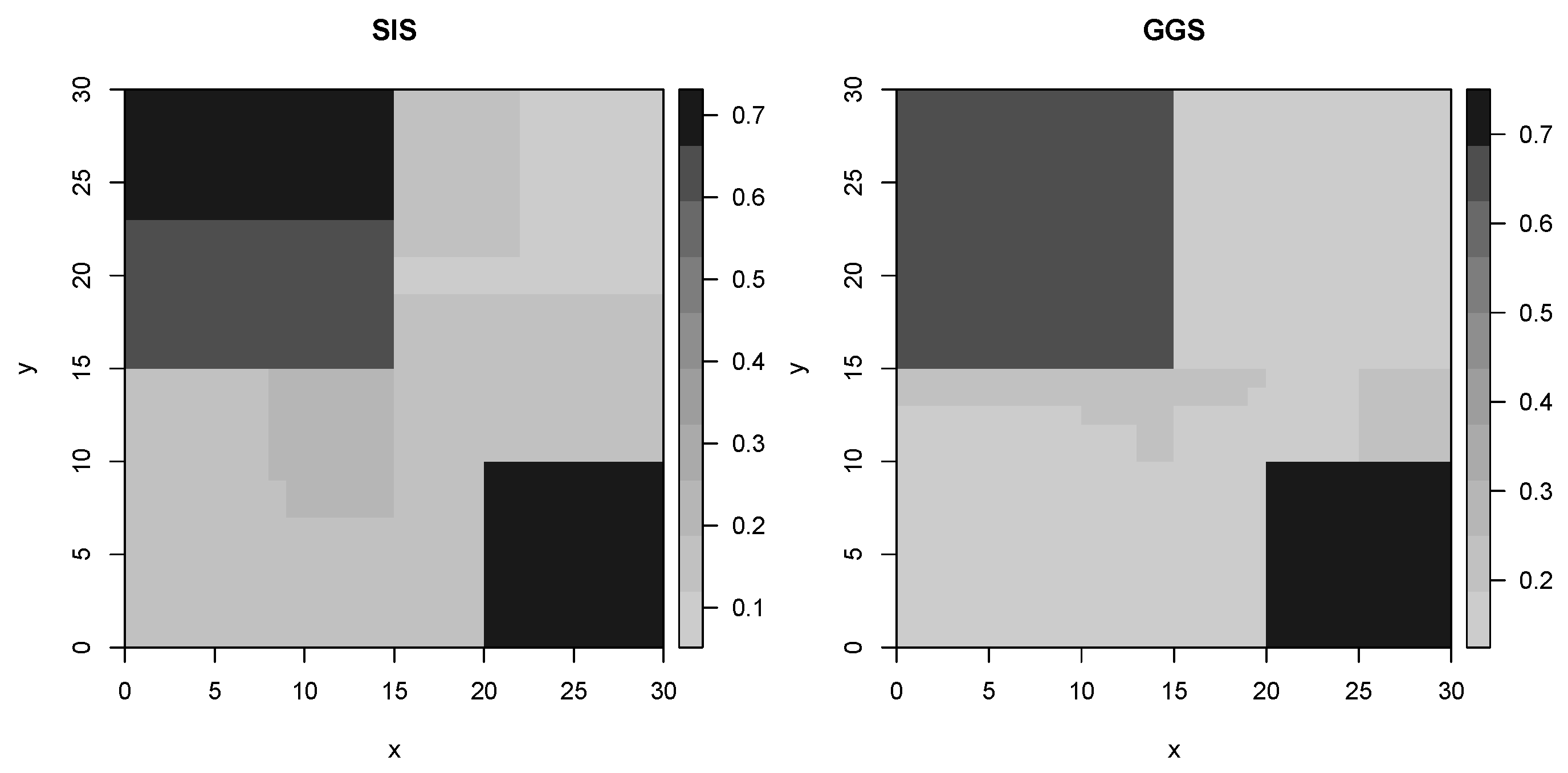
Figure 2 shows the true profile (left) of the data and the true parameters (right) which could be attributed to the fact that although the matrix was drawn from Bernoulli distributions with parameters given in Table 1, it is still artificially generated data and it is possible that the true profile may not be exactly the same as the Bernoulli parameters given in the table. In this example, we set as 100. The obtained profile from the GGS algorithm is an average of 175 draws which gives smooth configuration. We ran the algorithm for 1000 iterations and burn-in period of 100. According to the autocorrelation plot given in Figure 3, we use a thin size of 5 and the effective sample size for this example. That is, we take every 5th draw to obtain the average surface profile (an estimate of the posterior mean). Figure 4 shows the surface profiles obtained from the GGS and the SIS algorithms. We do not report a plot of log-likelihood versus iteration here since it is very similar to the corresponding plot given in Example 2. Our algorithm finds 10 domains at its convergence stage. Due to the nature of the SIS algorithm, it overestimates the number of domains and provides a noisy profile when we increase d (which decides the number of segments) to a large number, but the average profile explains the data very well. To make comparison easy, we use the same parameter values for both algorithms. Thus, the profiles obtained by the SIS algorithm is for and . For more details on the SIS algorithm for spatial segmentation and change-point problem, see [31,35]. The two plots are in excellent agreement with the true profile, supporting the fact that both methods produced only very small difference between their estimates and the true distribution.
The RMSE values for the SIS and the GGS are 0.0547 and 0.02435, respectively, indicating that the GGS algorithm produces a more accurate estimate compare to the SIS. Figure 5 shows the map of the standard error for the whole matrix in Example 1. The minimum, maximum and average values of the standard error are 0.0012, 0.0086 & 0.0031, respectively.
5.2. Artificial Data: Example 2
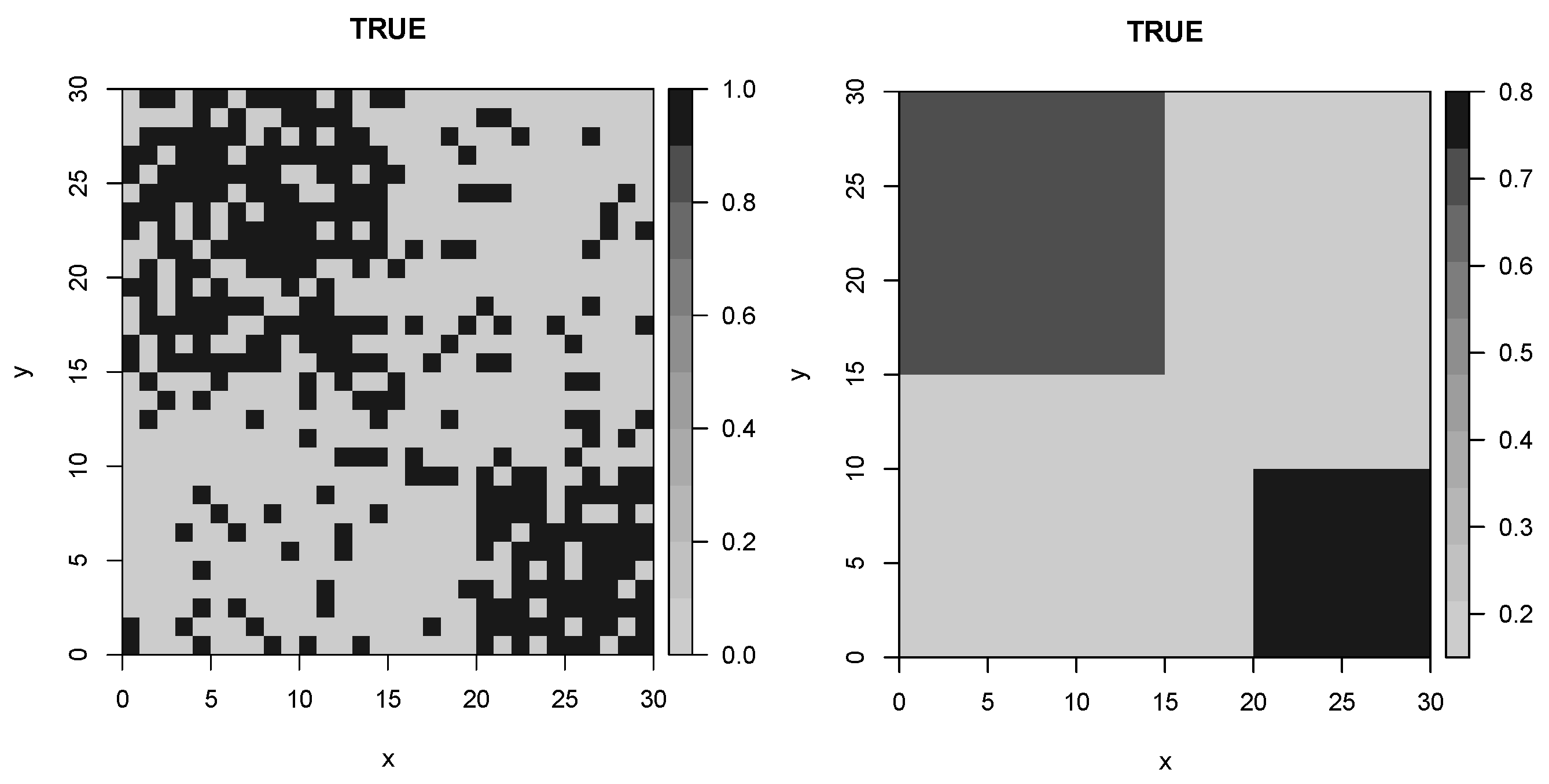
Figure 6 shows the true profile and the true parameters of the second artificial data. As in Example 1, we executed 1000 iterations of our algorithm (burn-in period of 100). In this example, the thin size is 6, and the effective sample size is 140. We take every 6th draw to obtain the average surface profile given in Figure 7. Figure 8 shows an estimated posterior standard error. The convergence of the GGS algorithm is evident in Figure 9. We do not report the autocorrelation plot here as it is very similar to Figure 3) in Example 1. For this example, the GGS algorithm finds seven domains; see Figure 9. The obtained profile by the SIS algorithm is for and . Table 2 illustrates the RMSE values and computational times for both GGS and SIS algorithms. The RMSE values are 0.06421 and 0.04419, respectively. The computational times for both SIS and GGS are for obtaining the given profiles in Table 2. We see that for the proposed GGS, the RMSE and the computational time are less than for the SIS.
5.3. Real Data
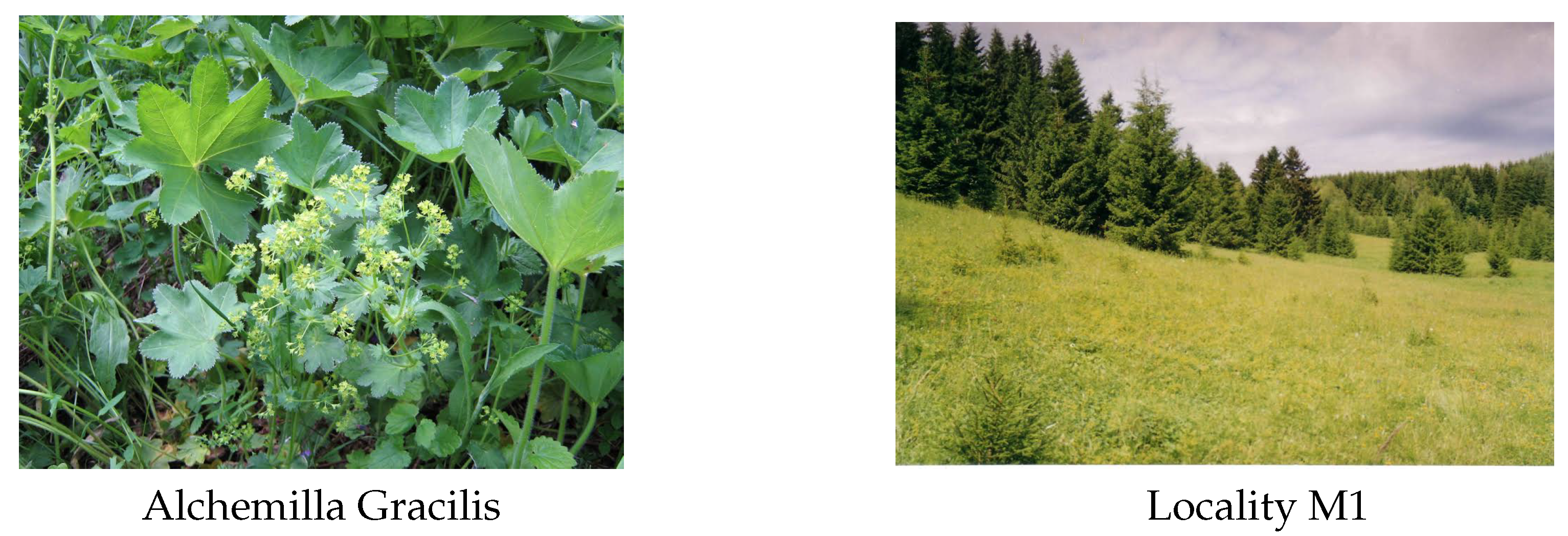
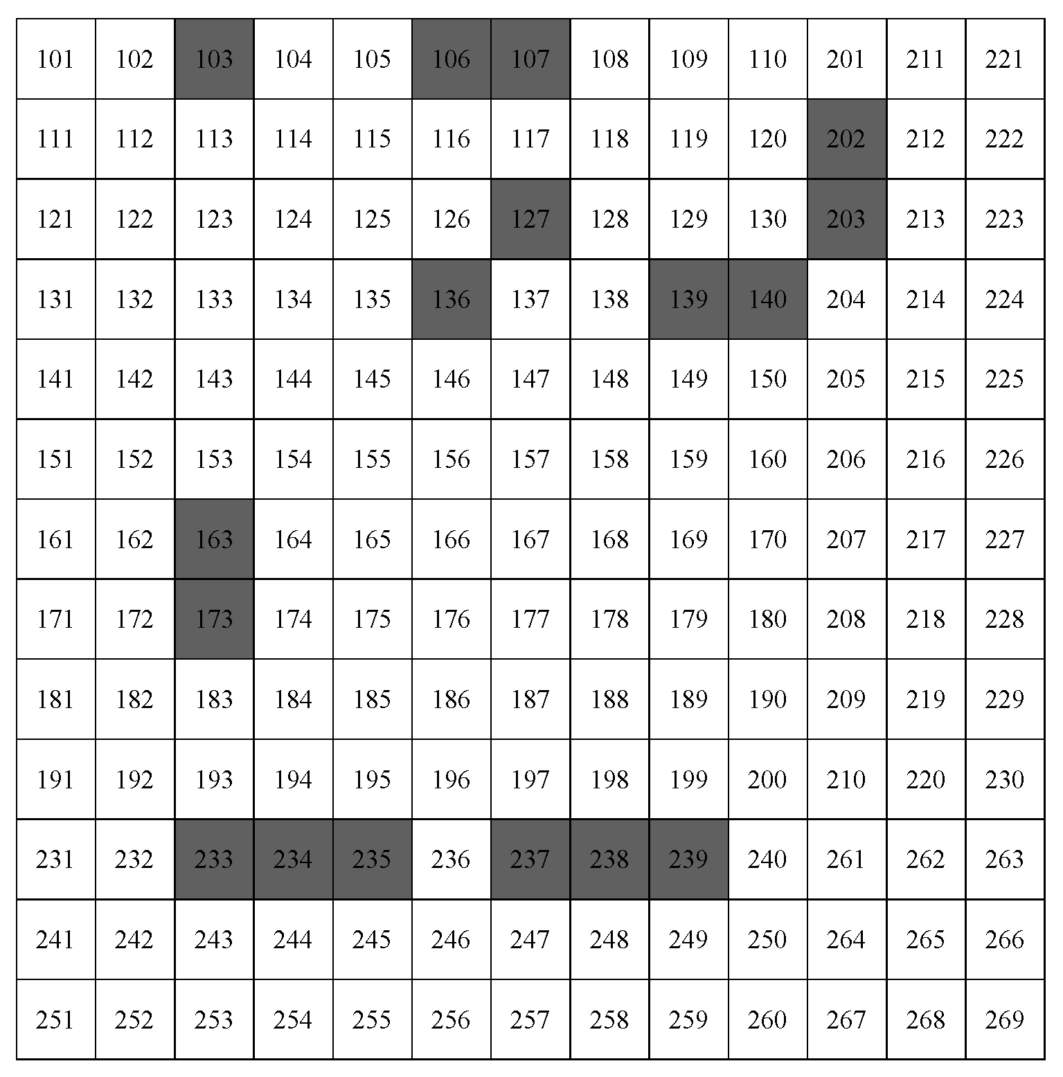
The third example uses a real plant data set [30]. The authors study Alchemilla plants and their microspecies growing within Eastern Europe with particular interest in the spatial distribution of the microspecies. The data were collected from 28 localities (habitats), which are characterised by different environmental conditions: bottomland meadow, dry meadow, fallow land, edge of mixed and coniferous forest. The plants were considered on square sites with the area of 1 . The surveyed area in localities varies from 2 to 169 . In this study, we consider locality M1, which has the largest number of sites. The 169 sites are numbered from 101 to 269.
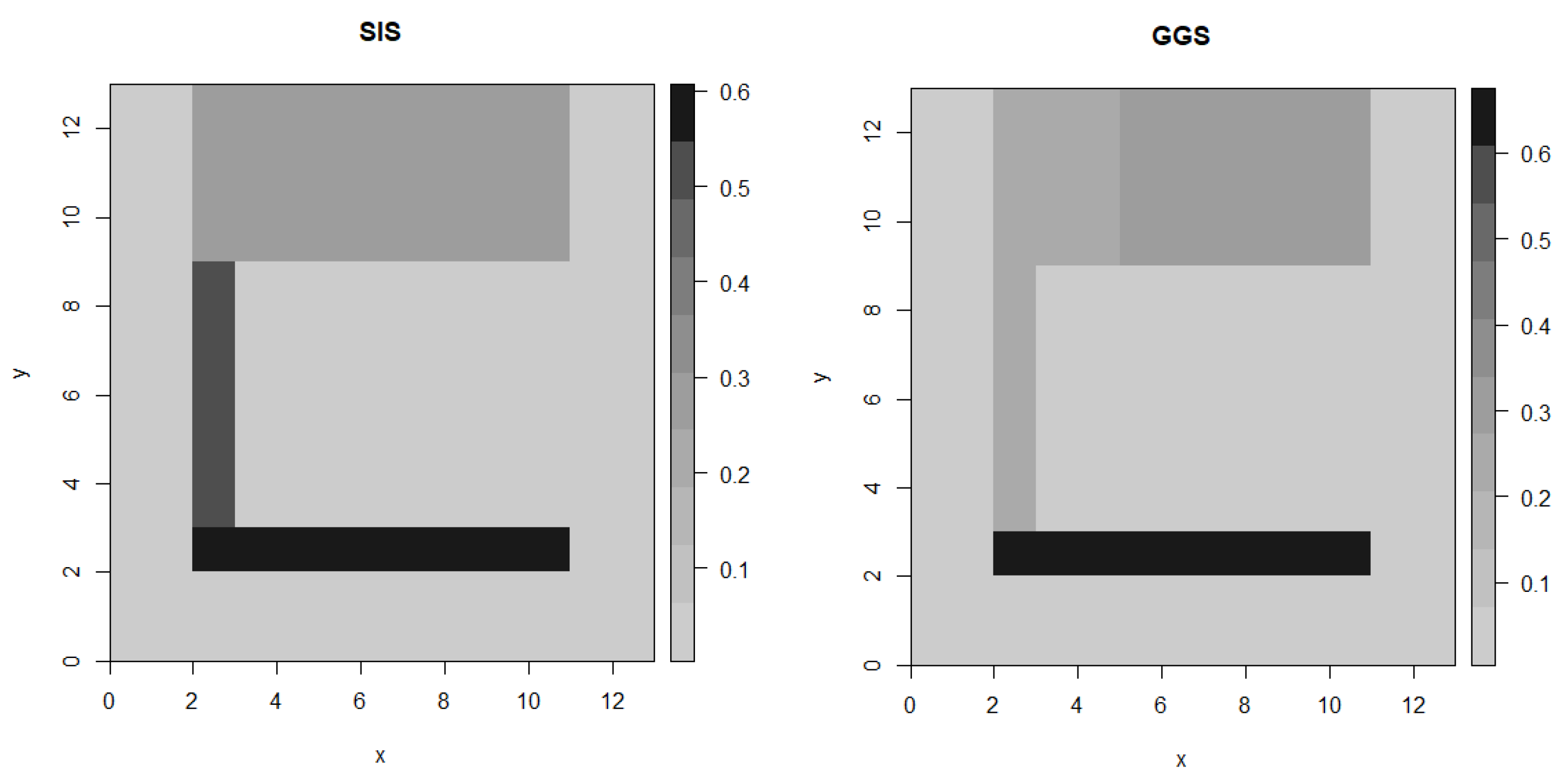
Figure 10 shows a particular type of plant Alchemilla and its study region. In Figure 11, a black cell indicates the presence of the plant, while a white cell means its absence. So we can consider a matrix encoded with zeros (white) and ones (black). As a consequence of considering a real data set, we do not know its true profile but we can still look for agreement between two algorithms. Since the size of the data set is relatively small, we set maximum number of domains to 10 for both algorithms. The obtained results given in Figure 12 is an average of 100 draws. The results for the real data seem reasonable looking at the data given, showing a general agreement between the GGS and the SIS.
6. Discussion and Conclusions
In this paper, we have developed an MCMC algorithm within the generalized Gibbs sampler framework to estimate the average surface profile explaining the heterogeneity of the spatial data observed over two-dimensional lattice. The Bayesian approach allows us to incorporate existing additional information by choosing an appropriate prior distribution and to make inference and interpretation of the results easier by estimating the posterior distribution. We have demonstrated the effectiveness of the proposed method in examples using both real and artificial data sets. For the artificial data sets, the profiles obtained by the GGS algorithm were in excellent agreement with both the SIS method and the true profile. Since we focus on estimating the posterior mean (average profile), we use the RMSE to compare the methods. Statistical information criteria like the Bayesian Information Criterion (BIC) can be used for comparison of models in the context of simulated annealing, when the posterior mode (the maximum of the posterior density function) is determined. When applying these two methods to the real presence-absence plant data set, comparable profiles were also obtained. The proposed GGS algorithm for spatial segmentation is effective in terms of mixing properties, accuracy and computational time. Overall, this paper has presented a promising new direction for spatial segmentation problem for different spatial models using change-point detection methodology. A possible limitation of this algorithm is that for very large scale datasets the computational cost may be high. However, this is an issue shared with all MCMC algorithms.
While we developed and compared two spatial segmentation algorithms, the development of new spatial segmentation algorithms based on other well-known statistical computational methods such as Cross-Entropy (CE) [25,36] and different MCMC algorithms [37] including the Reversible jump sampler is a matter of our further research. Developing a modified BIC and other information criteria for this problem to select the best model is also one of the future works.
Author Contributions
Methodology, G.S.; software, N.R.; validation, N.R.; formal analysis, N.R.; writing—original draft preparation, N.R.; writing—review and editing, G.S.; visualization, N.R.; supervision, G.S.; project administration, G.S. All authors have read and agreed to the published version of the manuscript.
Funding
This research received no external funding.
Institutional Review Board Statement
Not applicable.
Informed Consent Statement
Not applicable.
Data Availability Statement
Data is contained within the article.
Acknowledgments
The authors would like to thank the referees for their helpful remarks on the manuscript.
Conflicts of Interest
The authors declare no conflict of interest.
Abbreviations
The following abbreviations are used in this manuscript:
| BIC | Bayesian Information Criterion |
| GGS | Generalized Gibbs Sampler |
| MCMC | Markov Chain Monte Carlo |
| RMSE | Root Mean Squared Error |
| SIS | Sequential Importance Sampling |
References
- Chen, S.S.; Gopalakrishnan, P.S. Clustering via the Bayesian information criterion with applications in speech recognition. In Proceedings of the 1998 IEEE International Conference on Acoustics, Speech and Signal Processing, ICASSP’98 (Cat. No. 98CH36181), Seattle, WA, USA, 15 May 1998; pp. 645–648. [Google Scholar] [CrossRef]
- Tung, A.K.; Hou, J.; Han, J. Spatial clustering in the presence of obstacles. In Proceedings of the Data Engineering: 17th International Conference on IEEE, Heidelberg, Germany, 2–6 April 2001; pp. 359–367. [Google Scholar] [CrossRef] [Green Version]
- Gangnon, R.E.; Clayton, M.K. Bayesian detection and modeling of spatial disease clustering. Biometrics 2000, 3, 922–935. [Google Scholar] [CrossRef] [PubMed] [Green Version]
- Anderson, C.; Lee, D.; Dean, N. Bayesian cluster detection via adjacency modelling. Spat. Spatio-Temporal Epidemiol. 2016, 11–20. [Google Scholar] [CrossRef] [Green Version]
- Beckage, B.; Joseph, L.; Belisle, P.; Wolfson, D.B.; Platt, W.J. Bayesian change-point analyses in ecology. New Phytol. 2007, 11–20. [Google Scholar] [CrossRef] [PubMed]
- López, I.; Gámez, M.; Garay, J.; Standovár, T.; Varga, Z. Applications of change-point problem to the detection of plant patches. Acta Biotheor. 2010, 51–63. [Google Scholar] [CrossRef] [PubMed]
- Raveendran, N.; Sofronov, G. Binary segmentation methods for identifying boundaries of spatial domains. Comput. Sci. Inf. Syst. (FedCSIS) 2017, 3, 95–102. [Google Scholar]
- Tripathi, S.; Govindaraju, R.S. Change detection in rainfall and temperature patterns over India. In Proceedings of the Third International Workshop on Knowledge Discovery from Sensor Data, Paris, France, 28 June 2009; ACM: New York, NY, USA, 2009; pp. 133–141. [Google Scholar] [CrossRef]
- Helterbr, J.D.; Cressie, N.; Davidson, J.L. A statistical approach to identifying closed object boundaries in images. Adv. Appl. Probab. 1994, 831–854. [Google Scholar] [CrossRef]
- Wang, Y. Change curve estimation via wavelets. J. Am. Stat. Assoc. 1998, 441, 163–172. [Google Scholar] [CrossRef]
- Sfetsos, A.; Siriopoulos, C. Time series forecasting with a hybrid clustering scheme and pattern recognition. IEEE Trans. Syst. Mancybernetics Part A Syst. Hum. 2004, 34, 399–405. [Google Scholar] [CrossRef]
- Arbia, G.; Espa, G.; Quah, D. A class of spatial econometric methods in the empirical analysis of clusters of firms in the space. Empir. Econ. 2008, 34, 81–103. [Google Scholar] [CrossRef] [Green Version]
- Wang, J.; Chuangang, Y.U.; Juying, Z. Constructing the Regional Intelligent Economic Decision Support System Based on Fuzzy C-Mean Clustering Algorithm; Soft Computing; Springer: Berlin, Germany, 2019; pp. 1–9. [Google Scholar]
- Sofronov, G. A hybrid algorithm for spatial small area estimation under models with complex contiguity. In Proceedings of the 2013 IEEE Symposium on Differential Evolution (SDE), Singapore, 16–19 April 2013; pp. 25–30. [Google Scholar]
- Fan, C.; Nhien-An, L.; Tahar, K. Clustering approaches for financial data analysis: A survey. arXiv 2016, arXiv:1609.08520. [Google Scholar]
- Besag, J. Spatial interaction and the statistical analysis of lattice systems. J. R. Stat. Soc. Ser. B (Methodol.) 1979, 36, 192–236. [Google Scholar] [CrossRef]
- Sherman, M.; Apanasovich, T.V.; Carroll, R.J. On estimation in binary autologistic spatial models. J. Stat. Comput. Simul. 2006, 76, 167–179. [Google Scholar] [CrossRef]
- Wu, H.; Huffer, F.R.W. Modelling the distribution of plant species using the autologistic regression model. Environ. Ecol. Stat. 1997, 4, 31–48. [Google Scholar] [CrossRef]
- Moller, J.; Pettitt, A.N.; Reeves, R.; Berthelsen, K.K. An efficient Markov chain Monte Carlo method for distributions with intractable normalising constants. Biometrika 2006, 93, 451–458. [Google Scholar] [CrossRef] [Green Version]
- Hughes, J.; Haran, M.; Caragea, P.C. Autologistic models for binary data on a lattice. Environmetrics 2011, 22, 857–871. [Google Scholar] [CrossRef]
- Liang, F. A double Metropolis-Hastings sampler for spatial models with intractable normalizing constants. J. Stat. Comput. Simul. 2010, 80, 1007–1022. [Google Scholar] [CrossRef]
- Keith, J.M.; Kroese, D.P.; Bryant, D.A. Generalized Markov Sampler. Methodol. Comput. Appl. Probab. 2004, 6, 29–53. [Google Scholar] [CrossRef] [Green Version]
- Chen, J.; Gupta, A.K. Parametric Statistical Change Point Analysis: With Applications to Genetics, Medicine, and Finance; Springer Science & Business Media: Berlin/Heidelberg, Germany, 2011. [Google Scholar]
- Eckley, I.A.; Fearnhead, P.; Killick, R. Analysis of changepoint models. In Bayesian Time Series Models; Barber, D., Chiappa, A.T., Cemgil, S., Eds.; Cambridge University Press: Cambridge, UK, 2011; pp. 205–224. [Google Scholar]
- Priyadarshana, W.J.R.M.; Sofronov, G. Multiple Break-Points Detection in Array CGH Data via the Cross-Entropy Method. IEEE/ACM Trans. Comput. Biol. Bioinform. 2015, 12, 487–498. [Google Scholar] [CrossRef]
- Keith, J.; Sofronov, G.; Kroese, D. The Generalized Gibbs Sampler and the Neighborhood Sampler. In Monte Carlo and Quasi-Monte Carlo Methods; Keller, A., Heinrich, S., Niederreiter, H., Eds.; Springer: Berlin, Germany, 2006; pp. 537–547. [Google Scholar]
- Sadia, F.; Boyd, S.; Keith, J.M. Bayesian change-point modeling with segmented ARMA model. PLoS ONE 2018, 13, e0208927. [Google Scholar] [CrossRef]
- Phillips, D.B.; Smith, A.F.M. Bayesian model comparison via jump diffusions. Markov Chain Monte Carlo Pract. 1995, 215, 239. [Google Scholar]
- Green, P.J. Reversible jump Markov Chain Monte Carlo computation and Bayesian model determination. Biometrika 1995, 82, 711–732. [Google Scholar] [CrossRef]
- Sofronov, G.Y.; Glotov, N.V.; Zhukova, O.V. Statistical analysis of spatial distribution in populations of microspecies of Alchemilla L. In Proceedings of the 30th International Workshop on Statistical Modelling, Linz, Austria, 6–10 July 2015; Friedl, H., Wagner, H., Eds.; Statistical Modelling Society: Linz, Austria, 2015; pp. 259–262. [Google Scholar]
- Raveendran, N.; Sofronov, G.Y. Identifying Clusters in Spatial Data via Sequential Importance Sampling. In Recent Advances in Computational Optimization; Fidanova, S., Ed.; Studies in Computational Intelligence Springer: Cham, Switzerland, 2019; pp. 175–189. [Google Scholar]
- Geyer, C. Introduction to Markov Chain Monte Carlo. In Handbook of Markov Chain Monte Carlo; Brooks, S., Gelman, A., Jones, G.L., Meng, X., Eds.; Hall/CRC: Chapman, CA, USA, 2011. [Google Scholar]
- Keith, J.M.; Kroese, D.P.; Sofronov, G. Adaptive independence samplers. Stat. Comput. 2008, 18, 409–420. [Google Scholar] [CrossRef] [Green Version]
- Liu, S. Monte Carlo Strategies in Scientific Computing; Springer Science & Business Media: Berlin/Heidelberg, Germany, 2008. [Google Scholar]
- Sofronov, G.Y.; Evans, G.E.; Keith, J.M.; Kroese, D.P. Identifying Change-points in Biological Sequences via Sequential Importance Sampling. Environ. Model. Assess. 2009, 14, 577–584. [Google Scholar] [CrossRef]
- Evans, G.E.; Sofronov, G.Y.; Keith, J.M.; Kroese, D.P. Estimating change-points in biological sequences via the Cross-Entropy method. Ann. Oper. Res. 2011, 189, 155–165. [Google Scholar] [CrossRef] [Green Version]
- Algama, M.; Keith, J.M. Investigating genomic structure using changept: A Bayesian segmentation model. Comput. Struct. Biotechnol. J. 2014, 10, 107–115. [Google Scholar] [CrossRef] [Green Version]
Figure 1.
(a) shows the first iteration starting with a random vertical cut . (b) shows the second iteration where is moved to left and a new horizontal cut is inserted. We keep vertical and horizontal cuts seperately to avoid label switching problem. (c) shows the third iteration where and are moved to their new positions and a new horizontal cut is inserted. (d) illustrates possible movements of all cuts for the fourth iteration. The vertical cut ’s possible leftmost and rightmost movements are and , respectively. The horizontal cut ’s possible uppermost and downmost movements are and , respectively. Dotted lines inside the domain illustrate possible vertical and horizontal cuts if it is chosen to be inserted a new cut.

Figure 2.
Domains as determined by the true profile (Example 1).

Figure 3.
Autocorrelation curve (Example 1).

Figure 4.
Surface profiles as determined by the generalized Gibbs sampler (GGS) and the Sequential Importance Sampling (SIS) algorithms in Example 1.
Figure 4.
Surface profiles as determined by the generalized Gibbs sampler (GGS) and the Sequential Importance Sampling (SIS) algorithms in Example 1.

Figure 5.
Map of the standard error (Example 1).

Figure 6.
Domains as determined by the true profile (Example 2).

Figure 7.
Surface profiles as determined by the GGS and the SIS algorithms (Example 2).

Figure 8.
Map of the standard error (Example 2).

Figure 9.
The value of log-likelihood (top) and the number of cuts (bottom) for the first 1000 iterations (Example 2).
Figure 9.
The value of log-likelihood (top) and the number of cuts (bottom) for the first 1000 iterations (Example 2).

Figure 10.
Alchemilla Gracilis plant (left) and its habitat (right).

Figure 11.
Layout of sites in locality M1. The 169 sites are numbered from 101 to 269. If a site has a particular microspecies then it is colour coded black, otherwise it is white.
Figure 11.
Layout of sites in locality M1. The 169 sites are numbered from 101 to 269. If a site has a particular microspecies then it is colour coded black, otherwise it is white.

Figure 12.
Surface profiles as determined by the GGS and the SIS algorithms.


Table 1.
The parameters of the generated data matrix.
| Domains | Coordinates (Bottom Left to Top Right) | Probability () |
|---|---|---|
| Domain 1 | (0,0)–(30,10) | |
| Domain 2 | (1,10)–(8,20) | |
| Domain 3 | (8,10)–(22,15) | |
| Domain 4 | (8,15)–(22,20) | |
| Domain 5 | (1,20)–(30,30) | |
| Domain 6 | (22,10)–(30,20) |
Table 2.
The average running time and root mean square for the GGS and the SIS algorithms.
| Algorithm | RMSE | Computational Time (s) |
|---|---|---|
| GGS | 0.04419 | 30.2928 |
| SIS | 0.06421 | 34.5378 |
Publisher’s Note: MDPI stays neutral with regard to jurisdictional claims in published maps and institutional affiliations. |
© 2021 by the authors. Licensee MDPI, Basel, Switzerland. This article is an open access article distributed under the terms and conditions of the Creative Commons Attribution (CC BY) license (http://creativecommons.org/licenses/by/4.0/).
Share and Cite
MDPI and ACS Style
Raveendran, N.; Sofronov, G. A Markov Chain Monte Carlo Algorithm for Spatial Segmentation. Information 2021, 12, 58. https://0-doi-org.brum.beds.ac.uk/10.3390/info12020058
AMA Style
Raveendran N, Sofronov G. A Markov Chain Monte Carlo Algorithm for Spatial Segmentation. Information. 2021; 12(2):58. https://0-doi-org.brum.beds.ac.uk/10.3390/info12020058
Chicago/Turabian StyleRaveendran, Nishanthi, and Georgy Sofronov. 2021. "A Markov Chain Monte Carlo Algorithm for Spatial Segmentation" Information 12, no. 2: 58. https://0-doi-org.brum.beds.ac.uk/10.3390/info12020058
Note that from the first issue of 2016, this journal uses article numbers instead of page numbers. See further details here.