
The Image Classification Method with CNN-XGBoost Model Based on Adaptive Particle Swarm Optimization

1
School of Software, Shandong University, Jinan 250101, China
2
School of Computer Science and Technology, Shandong University of Finance and Economics, Jinan 250014, China
*
Author to whom correspondence should be addressed.
Information 2021, 12(4), 156; https://0-doi-org.brum.beds.ac.uk/10.3390/info12040156
Submission received: 5 March 2021
/
Revised: 29 March 2021
/
Accepted: 3 April 2021
/
Published: 9 April 2021
(This article belongs to the Special Issue Data Modeling and Predictive Analytics)
Abstract
:CNN is particularly effective in extracting spatial features. However, the single-layer classifier constructed by activation function in CNN is easily interfered by image noise, resulting in reduced classification accuracy. To solve the problem, the advanced ensemble model XGBoost is used to overcome the deficiency of a single classifier to classify image features. To further distinguish the extracted image features, a CNN-XGBoost image classification model optimized by APSO is proposed, where APSO optimizes the hyper-parameters on the overall architecture to promote the fusion of the two-stage model. The model is mainly composed of two parts: feature extractor CNN, which is used to automatically extract spatial features from images; feature classifier XGBoost is applied to classify features extracted after convolution. In the process of parameter optimization, to overcome the shortcoming that traditional PSO algorithm easily falls into a local optimal, the improved APSO guide the particles to search for optimization in space by two different strategies, which improves the diversity of particle population and prevents the algorithm from becoming trapped in local optima. The results on the image set show that the proposed model gets better results in image classification. Moreover, the APSO-XGBoost model performs well on the credit data, which indicates that the model has a good ability of credit scoring.
1. Introduction
Image classification which belongs to the main research content of image processing has a broad application prospect in many sciences, such as object recognition, content understanding and image matching. Support vector machine (SVM) [1], k-nearest neighbor (KNN) [2] and decision tree (DT) [3] are all typical machine learning methods applied in this field. These studies prove the effectiveness and reliability of machine learning applied in image classification. In essence, process of the image classification is regarded abstractly as the composition of feature extraction and feature classification: First, the model extracts significant features and helps the latter classifier distinguish features better. Second, the classifier accepts extracted features and identifies them effectively. Feature extraction is an important part of image classification system. In image classification task, extracted feature quality directly affects performance of classification. The previous classifications did not fully extract information from image feature until neural network (NN) was applied to image classification, and image classification quickly became an important research direction in this field. Theoretically, NN can approximate any complex function and effectively solve the problem of image feature extraction. Except for image classification, neural networks have made continuous breakthroughs in target detection [4,5], face recognition [6,7] and other fields. Among them, CNN is an efficient neural network learning model, whose convolution kernel in the convolutional layer plays an important role in the extraction of features. The features of images are extracted automatically by convolution, and hierarchical structure of CNN can learn high-quality features at each layer. Although CNN is considered as the one of most powerful and effective feature extraction mechanism, the traditional classifier lay of CNN cannot fully grasp the information of feature extracted, which as single classifier cannot perform well in the face of diverse and complex data features. On the basis of the “No Free Lunch” theorem [8], for different structures and characteristics of changeable data, the prediction accuracy is greatly limited by a single classifier. Ensemble learning combines multiple classifiers that process different hypotheses to construct a better hypothesis and obtain excellent predictions. Dietterich [9] explained three basic reasons for the success of ensemble learning from three mathematical perspective: statistics, calculation and representativeness. In addition, the bias variance decomposition analyzes the effectiveness of ensemble learning [10]. Kearns and Valiant [11] showed that weak classifiers can generate high precision estimates by integrating, as long as data is sufficient. These studies proved that ensemble learning has a better learning ability than a single classifier. Furthermore, Chen [12] proposed an advanced gradient boosting algorithm, the extreme gradient boosting tree (XGBoost), that has obtained good results in Kaggle data competitions. XGBoost has been widely used in image classification [7,13] and has good performance. Ren et al. [14] proposed an image classification method based on CNN and XGBoost. In this model, CNN is used to obtain features from the input, and XGBoost as a recognizer produces results to provide more accurate output. The experimental results on MNIST and CIFAR-10 show that the performance of this method is better than other methods, which verifies the effectiveness of the combination of CNN and XGBoost in image classification.
Good performance of models depends on the proper hyper-parameter settings. The hyper-parameters directly affect the structure of models and the performance of the model, so it is particularly important to tune the hyper-parameters appropriately. Generally, models rely on artificial experience tuning, which consumes a great deal of time and computing resources. Hyper-parameter optimization has been used to tune hyper-parameters to overcome the shortage of manual tuning. Most optimization of hyper-parameters performs in a continuous search space. Particle swarm optimization (PSO), originally proposed by Kennedy and Eberhart [15], is a computational intelligence technique. The original PSO algorithm was mainly designed for the optimization of a continuous space owing to the quantities describing the particle state and its motion laws being continuous real numbers. Song and Rama [16] proposed a XGBoost model combining the improved PSO algorithm to determine the relationship between tensile strength and plasticity and their influencing factors. The experimental results prove the effectiveness and reliability of the method. Le et al. [17] proposed a building thermal load forecasting and control model PSO-XGBoost. PSO optimizes the XGBoost model as predictor. The experimental results show that the proposed model is the most robust method for comparing the average absolute percentage error (MAPE), variance analysis (VAF) and other indicators of other models (XGBoost, SVM, RF, GP and CART) on the survey data of buildings. These studies prove the effectiveness of PSO to improve the performance of XGBoost learning algorithm. Therefore, PSO is more suitable for the hyper-parameter optimization. PSO finds the optimal solution through iteration, and it has a fast convergence speed. However, its disadvantage is that the states of the particles fall into a local optimum easily, thereby causing premature convergence. In response to this problem, we purpose the adaptive PSO (APSO). It uses the idea of clustering to adaptively divide the particle swarm into different populations and guide the populations by applying different update strategies. This enhances the diversity of particles and helps particles jump out of a local optimum. APSO is more suitable for the parameter optimization, and it improves the model prediction accuracy.
Based on the above, we propose a CNN-XGBoost based on APSO optimization for image classification. CNN is used as a feature extractor to automatically obtain features from the input, and the feature recognizer XGBoost receives the image features and then produces results; the parameter optimizer APSO is applied to optimize the structure of model to match feature, so the model gets accurate results.
The contributions of this paper are as follows:
Firstly, a novel two-stage fusion image classification CNN-XGBoost based on APSO is proposed. It both ensures CNN can extract image features fully and makes use of XGBoost to distinguish features effectively, so as to ensure high accuracy of image classification as a whole.
Secondly, bidirectional optimization structure is adopted, both CNN and XGBoost are optimized by APSO at the same time. For one thing, optimizing the CNN to extract deep features, so that the extracted features are more suitable for the decision trees XGBoost, and for another, optimizing XGBoost makes the structure of the model match the extracted features, so as to better understand the image features. Bidirectional optimization maintains the characteristics of the two parts themselves meanwhile allowing the two parts to combine more closely together, making the features of the image fully extracted to be used for classification.
Thirdly, the PSO algorithm is improved based on adaptive subgroup division. Two different learning strategies are adopted to update different types of particles, enhance the diversity of particle population and avoid the algorithm falling into local optimal which improves adaptive processing capability of model for image features and increases accuracy of classification.
The rest of the paper is organized as follows: Section 1 explains the related work on the methods used. Section 2 introduces the principle of the CNN-XGBoost based on APSO model. Section 3 describes the experimental setup. Section 4 reports the experimental analysis results. Section 5 describes supplementary experiment in detail. Finally, Section 6 concludes the paper and discusses future work.
2. Materials and Methods
In this section, we introduce the related content and principles about CNN, XGBoost and parameter optimization.
2.1. CNN
CNN was first proposed by Professor Yann LeCun et al. used for recognition and classification of handwriting digital images [18]. The two most important processes of CNN are convolution and down-sampling. Convolution is to extract features from data, while sampling is to reduce dimension of data. Compared with other neural networks, CNN has the characteristics of Local Connectivity, Weight Sharing and Pooling. Local Connectivity is inspired by characteristic of image space, which is the local pixel spatial connection that is relatively close while the pixel correlation far away is weak. Local Connectivity is achieved by convolution operations. Each neural unit processes only one part of the image and then summarizes the results of each part. Local Connectivity is equivalent to constructing a number of spatial localized filters which can obtain some salient features of the input. Computation and training difficulty of model are reduced through convolution. Weight Sharing is based on the reasonable assumption: “if a batch feature is valid for computation at one space location, it should be valid for computation at other locations”. Because the picture has its own inherent characteristics, some statistical characteristics should be roughly the same as others. It is made by each convolution filter (convolution kernel) sharing a matrix with the same weight. Weight sharing reduces the number of parameters and reduces the difficulty of calculation. The Pooling is the process of feature mapping. The input image is divided into a set of non-overlapping rectangles, and output is the maximum value based on these subregions by pooling. The pooling layer operates independently on each depth slice of the input and adjusts their spatial size. It reduces the size of the representation space gradually to reduce the number of parameters, thus reducing the memory footprint, the computation and controlling overfitting. A typical CNN consists of alternating convolution and sub-sampling layers and then turns into fully connected layers when approaching the last output layer. It usually adjusts all the filter kernels by back-propagation algorithm [19], which is based on stochastic gradient descent algorithm, to reduce the gap between the network output and the training labels. Overall, the convolution layer obtains the local features by connecting with local receptive fields. The pooling layer is a mapping feature layer which is used for pooling operation and completing the secondary extraction calculations. Each convolution layer is followed by a pooling layer, and the special twice feature extraction structure makes CNN have strong distortion tolerance on the input images.
2.2. XGBoost
XGBoost, developed by Chen and Guestrin [20], is a powerful methodology for regression as well as classification. It is applied as a group of winning programs from Kaggle machine learning competitions. XGBoost, based on the gradient boosting framework, constantly adds new decision trees to fit a value with residual multiple iterations and improves the efficiency and performance of learners. Unlike gradient boosting, proposed by Friedman [21], XGBoost uses a Taylor expansion to approximate the loss function, and the model has a better tradeoff bias and variance, usually using fewer decision trees to obtain a higher accuracy. Details of XGBoost are described below.
Suppose a given sample set has n samples and m features; it can be expressed as , where x is the eigenvalue, and y is the true value. The algorithm sums the results of K trees as the final predicted value, which is expressed as
F is the set of decision trees, as follows:
where is one of the trees, and is the weight of the leaf nodes. T is the number of leaf nodes, and q represents the structure of each tree, which maps the sample to the corresponding leaf node. Therefore, the predicted value of XGBoost is the sum of the value of the leaf nodes of each tree. The goal of the model is to learn these k trees, so we minimize the following objective function:
l is the loss of the difference between the estimated values and the true value yi; common loss functions include the logarithmic loss function, square loss function, and exponential loss function. Ω regularization is used to set the penalty of the decision tree, which can prevent overfitting. Ω is expressed as follows:
In the regular term, is a hyper-parameter that controls the complexity of the model, and T is the number of leaf nodes. is the penalty coefficient for the leaf weight , which is usually constant. and determine the complexity of the model and are usually given empirically. During training, a new tree is added to fit the residuals of the previous round. Therefore, when the model has t trees, it is expressed as follows:
Substituting (4) into the objective function (2) yields the function
Then, XGBoost carries out the Taylor expansion of the objective function, takes the first three terms, removes the high-order small infinitesimal terms, and finally transforms the objective function into
where is the first derivative, and is the second derivative of loss function respectively. The residual between the prediction score and yi does not affect the optimization of the objective function, so it is removed.
The iteration of the tree model is transformed into the iteration of the leaf nodes, and the calculated optimal leaf node score is . Where is and is , by substituting the optimal value into the objective function, the final objective function is obtained:
Overall, XGBoost adds regularization to the standard function as a result of the reduced model complexity. The first and second derivatives are applied to fit the residual error. This method also supports column sampling in both reducing overfitting and reducing computation. Therefore, more improvements lead to more hyper-parameters than the gradient boosting decision tree (GBDT). However, it is difficult to reasonably tune the hyper-parameters. A reasonable setting requires not only the prior knowledge of researchers and their experience in parameter tuning but also a great deal of time. Hyper-parameter optimization is an effective solution to this problem.
2.3. Parameter Optimization
The parameter is one of the most significant concepts in machine learning, and the training model essentially finds the appropriate parameters to achieve better results. The parameters are divided into model parameters and hyper-parameters. The model parameters are obtained by learning the distribution of training data, without the need for human experience. The definition of a hyper-parameter is that it is a higher-level concept about the model, such as its complexity or ability to learn. Having a set of good hyper-parameters improves the performance of learning models, so tuning is important for hyper-parameters. However, hyper-parameter tuning is subjective and relies on empirical judgement and trial-and-error approaches [22]. The hyper-parameter optimization algorithm overcomes the dependence of manual search on experience and trial and error. Common hyper-parameter optimization algorithms include grid search, random search and Bayesian optimization. Below is a brief introduction to them.
Grid search (GS): GS is, within a specified range for the hyper-parameters, a method that uses one step at a time to adjust the hyper-parameters through training and is found to be best with all validation methods. However, a GS cannot widely explore a hyper-parameter space because by increasing the iterations of the algorithm to give more opportunities for the number of hyper-parameters, the computational complexity of GS grows exponentially. Therefore, GS is not suitable for the optimization of models with many dimensions [23].
Random search (RS): RS samples a certain number of sets from a specified distribution by randomly sampling within a search range. The theoretical basis is that if the set of random sample points is large enough, the global optimal value or its approximation will be found.
Bayesian optimization [24] in tuning hyper-parameters was intended to optimize the objective function of sample points by being added to the objective function to update the posterior distribution; the calculation process of this algorithm is Gaussian and considers the information of the last hyper-parameter, then adjusts the hyper-parameter to improve the joint posterior distribution slowly. Bayesian hyper-parameter optimization assumes that there is a real distribution, and the noise of the hyper-parameter is mapped to a specific target function. Xia et al. [25] proposed the tree-structured Parzen estimator (TPE), which is a Bayesian optimization method of tuning the hyper-parameters of XGBoost; the results show that the model outperforms other models according to the evaluation measures. Guo et al. [26] used the improved gradient boosting machine (GBM) combined with advanced feature selection and Bayesian hyper-parameter optimization to establish the fitness evaluation model. The experimental results show that the model has higher evaluation accuracy than other models. Putatunda et al. [27] used Bayesian optimization tools Hyperopt, RS and GS to adjust the hyperparameters of XGBoost algorithm on six real data sets. The performance of these three hyper-parameter optimization techniques was compared in the experiment. The results show that Bayesian optimization performs better in precision and time than GS and RS. However, Bayesian optimization is established on the basis of the distribution of the independent prior and the idealized hypothesis that properties are independent of each other. This condition is difficult to attain in practical applications; the number of properties may be large, or the correlation between the properties may be high, thereby causing performance degradation.
2.4. PSO
PSO simulates a bird in a flock by designing a massless particle that has only two properties: the speed, which represents how fast it moves, and position, which guides the direction in which it moves. Each particle determines the optimal solution in the search space of an individual and stores it as the current individual extremum. According to the current individual extremum of all the particles, to obtain the current global optimal solution, the whole particle swarm adjusts its speed and position. The process of PSO is as follows: First, initialize the particle swarm; then, evaluate the particles, calculate the adaptive value, search for individual extrema and find the global optimal solution. Finally, modify the speed and position of the particles.
The standard PSO algorithm is as follows: Suppose that in a d-dimensional search space, there is a population of m particles represented as , where the particles are expressed as . At a set time t, the characteristic information of is the position , speed , personal best position , and global optimal position . Then, the speed and position information of the particle can be updated at time by the following formula:
is the inertia weight that maintains an effective balance between global exploration and local exploration, and and are the learning factors (random numbers in a uniform distribution function) that adjust the step length of the direction of motion to the position of the particle and the direction of the global best position, respectively. To avoid a blind search by the particle, its speed and position are generally limited to and .
3. CNN-XGBoost Based on Apso Model
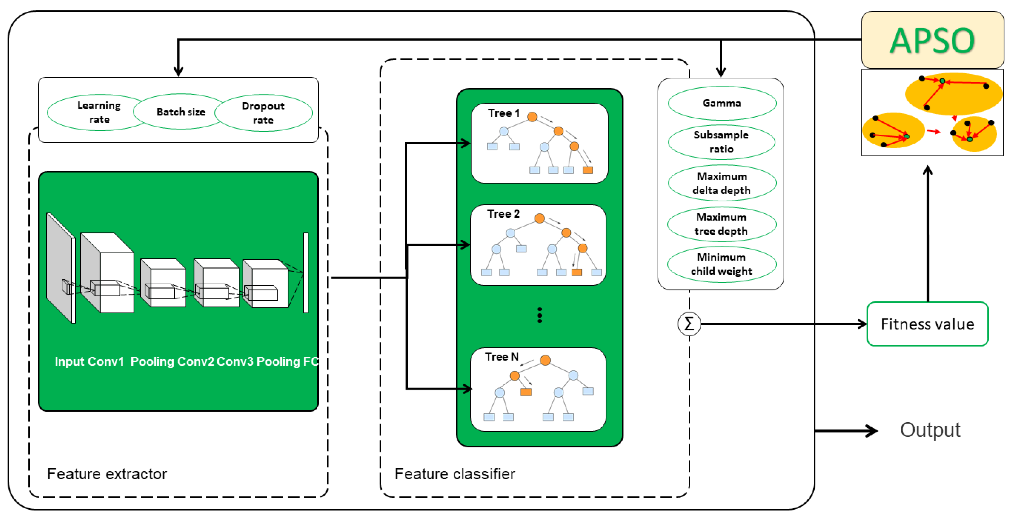
In this section, the image classification CNN-XGBoost based on APSO is shown in detail (see Figure 1). The model is divided into two parts: feature extractor, feature classifier. First, feature extractor CNN extracts features from the image data set. Second, XGBoost takes the features to train and classify. Then, according to the fitness value obtained from the model, the improved optimizer APSO is used to optimize the overall framework of CNN and XGBoost. Finally, when termination conditions are met, the optimal value of the hyper-parameter obtained by APSO is used to establish the image classification model. The process is described below: Section 2.1 describes the image feature extractor. Section 2.2 states the feature classifier XGBoost. Section 2.3 introduces the hyper-parameter optimizer APSO. Finally, the overall framework of the model is summarized.
3.1. Feature Extractor
Since CNN once again led the development of artificial intelligence, the AlexNet proposed by Krizhevsk et al. [28] has greatly improved the accuracy of image recognition. While the performance of these algorithms is improved, the calculation time is longer and longer with the increase of the model depth. This paper aims to explore the better combination between feature extraction ability of neural network and classification of decision tree; we design the lightweight model. Considering the model calculation, the specific structure of CNN for image classification consists of 7 layers: 1 input layer, 3 convolution layers, 2 pooling layers, 1 full connection layer. Configuration of feature extractor architecture is shown (see Table 1).
Steps of feature extractor as follow:
- 1
- Initialize the parameters of network.
- 2
- After convolution calculating, feature data obtained though each activation layer and pooling layer.
- 3
- The feature map forms a one-dimensional vector being processed by a fully connected layer.
- 4
- Vectors initialized into a new training data set which is used for predicting by subsequent classifier.
3.2. Feature Classification
In this section, XGBoost uses BP algorithm to train the features extracted by CNN, to obtain a tree structure suitable for feature classification.
The tree structure directly affects classification performance of XGBoost. Objective function formula (8), also known as structure score. The value of the function represents the quality of the tree structure. In order to minimize the value of the objective function, one of the key tasks of tree learning is to find the best node partition. By using the score in the instance sets of left nodes and right nodes after the split, the candidate segmentation is evaluated. Based on the evaluation, the optimal node is found to be divided, and finally, a tree with the optimal structure suitable for the data classification is found.
3.3. Adaptive PSO
In this section, we introduce PSO improved by adaptive learning strategies. In the process of searching, groups are adaptively divided into subgroups according to the particle distribution. In each subgroup, we use two different learning strategies to guide the search directions of two different types of particles. The search process stops when a global optimal value is found or a termination condition is met.
Relevant studies have shown that the diversity of the population is the key to avoiding the premature convergence of PSO; the core guiding principle of the algorithm is clustering [29]. According to the distribution of each particle, the fast search clustering method [30] is adopted to perform the adaptive division of the population into several subgroups. This method can automatically discover the data set samples’ class cluster centre. The basic principle is that the centre of the class cluster has two basic features: The first is that it is surrounded by points with lower local density, and the second is that it has a greater distance from points with a higher local density. Therefore, for a population of N particles , the two properties and are defined for each particle. , the distance between the local density of the particle and a higher local density of particles, is defined as follows:
where is the Euclidean distance of particles between , and and is the truncation distance. The truncation distance is , where R represents the proportion and M indicates that the matrix contains values, where N represents the number of particles. It can be seen that is the distance corresponding to the th value of . (11) gives the expression of the distance , representing the minimum distance from particle i to other particles that have a higher :
For the maximum local density of the sample, .
According to Equation (10), if the density of particle is the maximum, is much larger than the distance of its nearest particles. Therefore, the centre of the subgroup consists of particles that have an unusually large distance and a relatively high density as well. In other words, the particles with larger and values are selected as the centre of the cluster. According to the above idea from [30], the formula is used to filter out particles that may become cluster centers. We arrange the values in descending order, then use the truncation distance to filter out the cluster centers from the order. Because the value of the top particle is more likely to increase exponentially than those of the other particles, it is distinguished from the value of the next particle. Referring to [30], R is set to be between 0.1 and 0.2. Through a parameter sensitivity analysis, we found that the value of the distribution parameter has no effect on the performance of the particle swarm algorithm. The default value in this article is 2. The cluster centre is obtained by dividing by the truncation distance after placing the other particles in subgroups where the denser is larger than the of and the is the closest to the of .
The particles of each subgroup are divided into ordinary particles, and local optimal particles based on the result of the division of subgroups. Under the primary guidance of the optimal particles, the ordinary particles exert their local search ability, and the updated formula is given as (12).
where is the inertia weight, and are the learning factors, and are uniformly distributed random numbers in the interval , is the best position of particles, and is the current best position of particle in the subgroup c. To enhance the exchange of information between subgroups, the local optimal particles are mainly updated by integrating the information of each subgroup. The update formula is as follows (see (13)), where C is number of subgroups.
Ordinary particles search for local optimality, but more importantly, they are used as the medium for information exchange between subgroups to modify the direction of population search and further improve the population diversity. In the same subgroup, unlike a learning strategy that causes too many particles to be gathered locally, the learning strategy integrates the information of the locally optimal particles from different subgroups to obtain more information and help avoid local optima. In addition, learning too much information may lead to the direction of the update being too fuzzy, which may counteract the convergence of particles. Considering that the local optimal particles have the maximum probability of finding the optimal solution in the subgroup, valuable guidance for the optimal solution is provided by their information. Therefore, the of each subgroup uses the average information to guide the local optimal particle update (see (13)). The transmission of the optimized information in the subgroups can be improved by this approach, the population diversity can be further increased, and particles can be prevented from falling into local optima.
3.4. Training the Model
First, the hyper-parameters of CNN (including the learning rate, batch_size, dropout) and the hyper-parameters in the XGBoost model (including the maximum tree depth, subsample ratio, column subsample ratio, minimum child weight, maximum delta step and gamma-delta) are the optimization targets, and the position of each particle is randomly initialized in the hyper-parameter search space. Second, the particles are divided into adaptive populations. This step is achieved by calculating the local density of the particles and the distances to the particles whose local density is higher. According to the value determined by the position of the particle, we assign the hyper-parameters of the model and bring the verification data into the model for prediction. Finally, the loss function on the verification data set is the fitness function of the particles. The simplified description of credit scoring is a two-category problem. If the labels of the positive and negative samples of credit data are defined as /, the logistic loss function is defined as
where p is the predictive value, and y represents the actual value. In this paper, because our model labels are 0 and 1, the logistic loss is as follows:
The particles are divided into ordinary particles and optimal particles in accordance with the fitness value. Different update strategies update the information of the corresponding particles, and the algorithm checks whether the termination condition is reached; if so, we obtain the optimized value. If not, based on the positions of the particles, the model reclassifies the population again, calculates the fitness value, and updates the position information of each particle until the termination condition is reached. Finally, the optimal hyper-parameters are used to construct the model, and the training and prediction are carried out through the data.
The algorithm steps are as follows:
- Divide the data sets, train the data for the training model, verify the data for prediction. Initialize the adaptive PSO algorithm. Subgroups of the particle swarms are divided according to Equations (10) and (11).
- Take the logistic loss function as the fitness value, and calculate the fitness value of each particle according to (15). Build the model with the corresponding hyper-parameters determined by current best particle. Training and prediction of data sets, and the fitness value is updated by the loss function given.
- Determine the position of the global optimal particle and the local optimal particle according to the result of the population division and the fitness values of the particles.
- According to (12) and (13), update the positions of the ordinary particles and locally optimal particles, respectively.
- Judge whether to terminate. If the termination condition that iterations is met, return the optimal value of the hyper-parameter; otherwise, return to 2.
- Obtain the optimal hyper-parameters to build the CNN-XGBoost model and calculate the indexes.
4. Experimental Setup
In this section, we evaluate the performance of CNN-XGBoost model by experiment. First, image sets are introduced. Second, we describe the structure setting parameters of the CNN. Finally, the experimental results are analyzed.
4.1. Image Sets
In the image classification experiment, experiments were carried out on three data sets: MNIST [31] and CIFAR-10 [32]. CIFAR-100. These three data sets are widely used and are specifically used to study the performance of image classification methods. MNIST is a classified dataset of handwritten numbers 0 to 9. The images in the CIFAR-10 data set contain ten categories of natural objects. In CIFAR-10, there are significant differences in the positions and proportions of objects within categories, as well as in the colors and textures between categories. The CIFAR-100 data set is similar to CIFAR-10; it has 100 classes, each containing 500 training images and 100 test images. The 100 classes in CIFAR-100 are divided into 20 superclasses. Each image comes with a tag which is “fine” tag or “thick” tag (superclass) (see Table 2).
4.2. Model Setting
This section mainly describes the optimized hyperparameters in the framework model and their optimization space (see Table 3).
5. Results
Average accuracy (ACC) is one of the most widely used evaluation indexes for classification evaluation. It represents the overall performance of the model and reflects the overall level of classification ability. In order to test the performance of the image classification model proposed in this paper, we evaluate it on the above three databases. All methods are trained on the original training data set. The classification accuracy results are shown in Table 4.
We first compared the MNIST dataset with advanced methods. It includes three combination methods, DLSVM [33], SAE-CNN, CNN-SVM, and two control methods, CNN, PSO-CNN-XGBoost. PSO-CNN-XGBoost represents the CNN-XGBoost model optimized by ordinary PSO, and the other two represent high-performance methods: CIDBM [34], PCAnet [35]. It can be seen from the table that the performance of our model is better than other methods on MNIST. Compared with CNN, it reflects the superiority of the two-stage model. Compared with the combination method, our model shows obvious advantages. The reason is that the ensemble classifier XGBoost understands image features better than other classifiers, and it is more compatible with CNN due to stronger classification performance. Compared with the control model PSO-CNN-XGBoost, our model has a significant improvement. It shows that APSO optimizes the hyperparameters of the overall framework to promotes the integration of the two parts, which enables the model to adaptively adjust the framework to grasp image features and improves classification accuracy. Our performance is also better than CDBM and PCAnet, further showing the good performance of the model.
We also compared the image classification methods on the more complex CIFAR-10 dataset. Those compared models include 2 combined models mentioned, 2 control models and 4 high-precision models: DLSVM, Maxout Networks [36], NIN [37] and ML-DNN [38]. It shows from the table that compared with other models, our model has the highest accuracy on CIFAR-10, reaching 91.98%, but its advantages are not obvious from the most advanced model: Our test result is only 0.10 higher than ML-DNN. Ours is significantly improved compared with the control PSO-CNN-XGBoost. It shows that the improvement of APSO parameter optimization is obvious, which due to the effectiveness of bidirection optimization form makes the two parts more closely integrated. The optimization mechanism optimizes the two parts of the model as a whole, integrates the learning objectives, and makes the whole model more suitable for image classification tasks. Compared with the combined method CNN-SVM, our model has a huge lead over other models, which further demonstrates the combination of CNN, and XGBoost is even more powerful in image classification. In general, our model is also competitive on the more complex image data set CIFAR-10.
In order to explore the performance of our model on more complex data sets and further illustrate the generality of ours, it is compared with other representative methods on the CIFAR-100. It can be seen from the Table 4 that PSO-CNN-XGBoost is slightly better than NIN on ACC. The CNN-XGBoost model under APSO tuning surpasses other methods and achieves the highest accuracy rate, which indicates that APSO adopts an adaptive strategy to guide the particle search well, to avoid falling into the local optimal situation to a certain extent. The APSO makes the framework extracts and utilizes image features fully to improve the classification accuracy. In general, our model architecture can meet the needs of more complex data sets and perform well. The model has good generality.
6. Additional Experiments
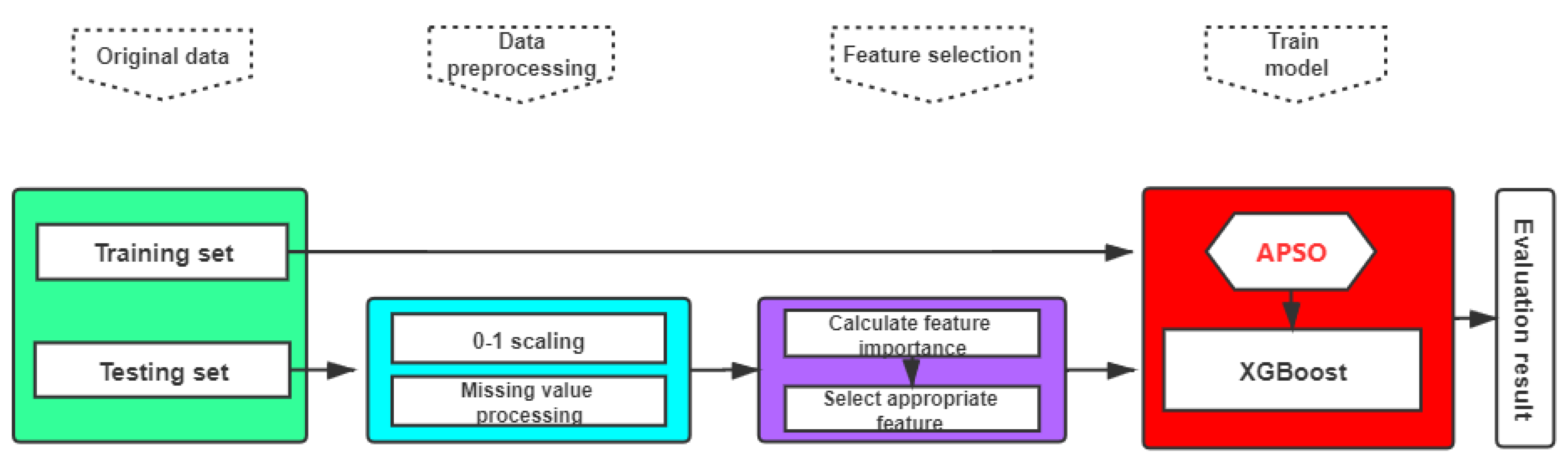
To further explore the performance of the model in terms of classification, we use XGBoost model optimized by APSO to build credit scoring model. First, to eliminate the errors caused by data that have self-variation or large differences in values, we preprocessed the original credit data. Then, we carried out feature engineering, which aims to extract the features from the original data that are maximally useful. In the final step, the model is built with the selected features and optimized hyper-parameters tuned by adaptive PSO, and test data tokens are used to evaluate the trained models.
The model is divided into three parts: data preprocessing, feature engineering and model training. First, the data preprocessing involves standardized data sets and marked missing values. Second, the feature engineering is based on the score of feature importance that is obtained from the initial hyper-parameter model. According to the rank of the feature importance, redundant features are removed. Finally, according to the selected features and hyper-parameters tuned by APSO, the model is built. The flow chart is shown in Figure 2. The process is described in detail below.
6.1. Data Sets
In this section, the performance of the model is verified by UCI credit data sets. Two credit data sets, German and Austrian, from the UCI machine learning repository are used. In addition to the above data sets, P2P credit data from two platforms (Lending Club in the US and We.com in China) were also used to verify the effectiveness of our model in providing decision support for P2P lending businesses and to verify the generalization of the model (see Table 5).
6.2. APSO-XGBoost
6.2.1. Data Preprocessing
Data preprocessing is divided into two steps: data standardization, namely, 0–1 scaling, and missing value processing. Although the tree-based algorithm is not affected by scaling, feature normalization can greatly improve the accuracy of classifiers, especially those based on distance or edge calculations. Therefore, the standardization of data sets in data preprocessing makes the model more accurate and persuasive. The training set is described as , where represents an m-dimensional eigenspace, represents the target value, represents poor application, and represents good application. If x is a certain feature, it is calculated by 0–1 scaling as follows:
where expresses the standardized value. Credit data often have missing values. XGBoost comes with its own sparsity segmentation algorithm, which can learn the best way to deal with missing values and is more suitable for modeling than traditional methods of dealing with missing values. If there are outliers and noise in the data, standardization can indirectly avoid the influence of outliers, and centralization can deal with extreme values.
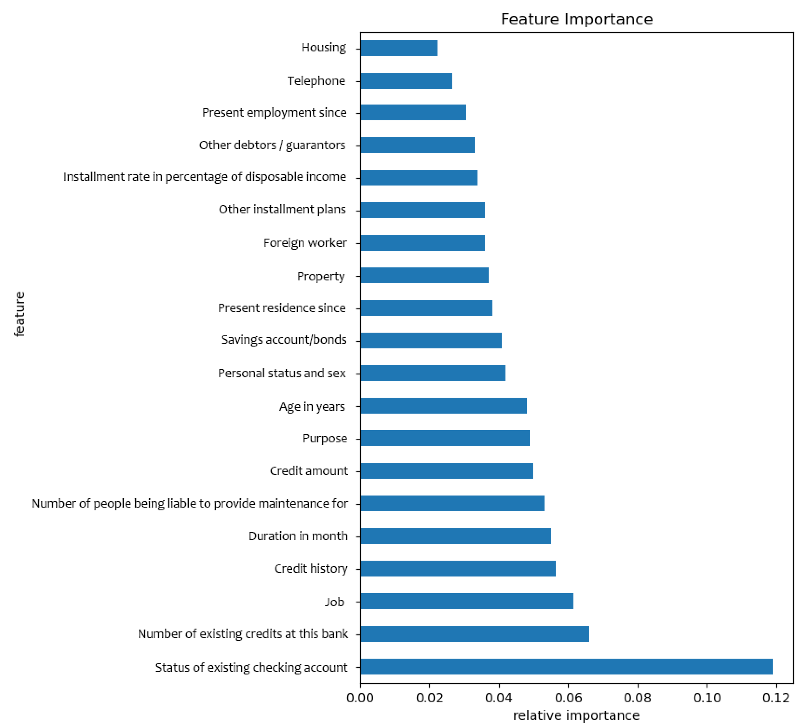
6.2.2. Feature Selection
At first, the score of the relative feature importance with the initial hyper-parameter is calculated, and the redundant features are discarded by the feature selection algorithm. The importance of feature selection lies in eliminating redundant features, highlighting effective features, improving the calculation speed and eliminating the influence of adverse features on the prediction results. An example as shown in Figure 3, it is the relative feature importance of the German credit dataset on XGBoost model.
6.2.3. Feature Engineering
Feature engineering selects important characteristics and removes irrelevant features to build a model. It can greatly reduce the dimension disaster problem, improve the operational efficiency, reduce the difficulty of learning tasks, make the model simpler and reduce the computational complexity.
By calculating the importance of the features, features that are more favorable to the model are selected. We choose the gain as the feature importance property as normal. XGBoost adopts the stochastic fractal search (SFS) algorithm according to the rank of the importance of the features and adds features into the data set to form subsets one by one. Under the default hyper-parameter of XGBoost, the subset that minimizes the logistical loss is selected as the subset of the features after 10-fold cross-validation.
6.2.4. Training the Model
To make the hyper-parameter accord with the training data set as much as possible, we use cross-validation on the data set. We tested several cross-validation methods. From many experimental results, we ultimately decided to use 10-fold cross-validation to divide the data sets. Except the feature extractor, the model is consistent with the image classification model steps: First, the hyper-parameters in the XGBoost model are the optimization targets, and the position of each particle is randomly initialized in the hyper-parameter search space. Second, the particles are divided into adaptive populations. This step is achieved by calculating the local density of the particles and the distances to the particles whose local density is higher. According to the value determined by the position of the particle, we assign the hyper-parameters of the XGBoost model and bring the verification data into the model for prediction. Finally, the loss function on the verification data set is the fitness function of the particles.
6.2.5. Baseline Models
To verify the performance of the model, we divided the baseline models into three groups: the traditional machine learning group, the integrated learning group, and the XGBoost group. The traditional machine learning group is DT, LR, NN, SVM, and RF; the ensemble learning group is AdaBoost, AdaBoost-NN, Bagging-DT, Bagging-NN, and GBDT; the XGBoost group is XGBoost-GS, XGBoost-RS, XGBoost-TPE, PSO-XGBoost and APSO-XGBoost. The baseline models are described in Appendix A.
6.2.6. The Evaluation Scale
When the label of sample is 0, the loan application is judged as a default state, indicating that the borrower failed to pay off the loan in time, and his credit is not good; when the sample label is 1, the loan application is non-default, indicating that the borrower fulfills the repayment agreement and he has good credit. In credit scores, the average accuracy is one of the most popular evaluation indices and represents the overall performance of the model. To better explore the ability of the model to distinguish between non-default and default applications, type I errors and type II errors in the confusion matrix are often used to evaluate the models to predict their performance in detail. A type I error is a default loan application being wrongly classified as a non-default. Conversely, a type II error is when a non-default is misclassified as default. and in the confusion matrix (see Table 6) represent the numbers of correctly classified good borrowers and bad borrowers, respectively. and represent the numbers of misclassified loan applications.
The formulas are defined as follows:
The average accuracy (ACC):
The type I errors:
The type II errors:
The Brier score (BS) measures the accuracy of the predicted probability and is the calibration of the prediction performance. The BS ranges from 0 to 1, and the interval value represents probabilistic predictions from perfect to poor. The BS is defined as follows:
where N is the number of samples. and denote the probability prediction and the true label of sample i, respectively.
The F1-score takes into account both precision and recall of classification models. It is the harmonic average of these two indicators, and it ranges from 0 to 1.
where precision is the proportion of positive samples in positive cases, it is defined as
And recall is the proportion of predicted positive cases in the total positive cases; it is defined as
6.3. Comparisons among Hyper-Parameter Optimization Methods
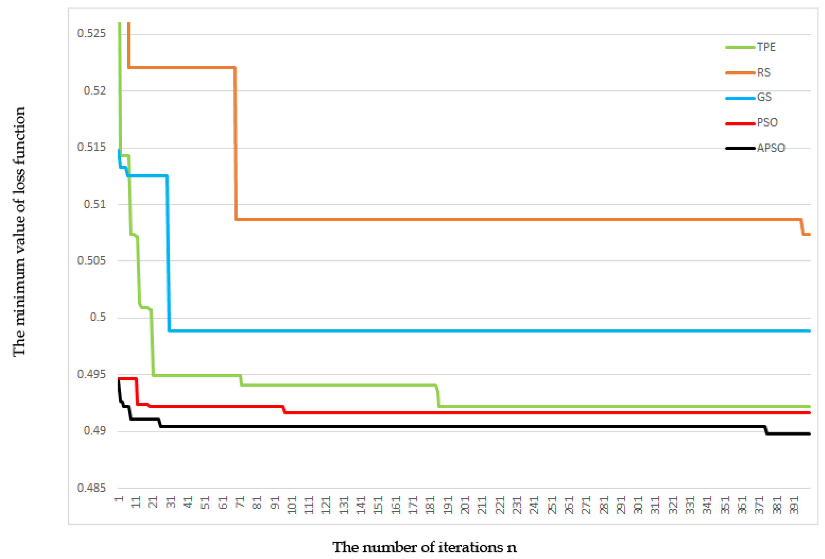
To demonstrate the performance of the tuning strategies, Figure 4 shows the convergence curves of average loss function of parameter optimization methods over four credit data. The ordinate represents average minimum value of loss function; the abscissa represents number of iterations. It can be seen from the figure that the convergence speed of GS and RS is slower. TPE converges faster, and its result is better than GS and RS. The value of the loss function of PSO is slightly lower than that of TPE, but the convergence speed of PSO is much faster. PSO and APSO have the fastest convergence speed among the parameter optimization methods. PSO has entered the convergence state early, which leads to its unsatisfactory final error rate and failure to find the global optimal value. APSO gets the best performance among all the converging performance. APSO still continues to decline after some iterations, indicating that the optimization mechanism helps subgroups increase diversity, prevents local particles from clustering, and helps particles to find the local optimal value.
6.4. Discussion
The ACC is one of the most mainstream and intuitive indicators. The ACC indicates the overall prediction ability of the model. In the German data set (see Table 7), the APSO-XGBoost model obtained the best value, 77.48%, on ACC, which is 1.37% higher than the best performance of the single classifier LR and is 1.37% and 1.16% higher than the best ensemble classifier GBDT in the group. APSO-XGBoost model has obvious improvement over PSO-XGBoost in each indicator. The reason is that when the APSO optimizes the hyper-parameter of XGBoost, the particle swarm easily jumps out of the local optimum and continues to find better values. Hyper-parameters that better match the fitness value give XGBoost a better tree structure, which makes the model prediction accuracy higher. Although the single classifier NN and Bagging-NN perform best in terms of type I error, our model has better results in terms of the other three indicators. APSO-XGBoost performs better in F1-score than other models, indicating that the model can still have more accurate prediction performance than other models under data imbalance.
For the Austrian data set (see Table 8), the ACC of APSO-XGBoost is 1.15% higher than the best-performing single classifier LR and 0.51% higher than the best-performing ensemble classifier RF. Because the numbers of positive and negative samples in the data set are very close, the error distribution of most models is balanced in general, and a few models have an uneven situation. In credit scoring, a high type I error rate guides institutions to adopt a more stringent mechanism to identify more applicants who have a possible default risk and reject them to reduce the risk of bad debt. The XGBoost group performs best in terms of the balance of the error distribution. This shows that the XGBoost classifier is well optimized. The type I error rate of our model ranks second only to that of the single classifier LR model, 11.80%. However, the error distribution of LR is uneven, and its type II error rate is the worst. The model evaluates more good applicants as bad, resulting in a higher type II error rate. In contrast, the error distribution of our method is more balanced than LR because the adaptive particle swarm can optimize multiple hyper-parameters at the same time, which ensures that the tree structure of the model screens both false positive rates and false negative rates. In terms of the BS, our model achieves the best score, 0.086.
For the P2P-LC data set (see Table 9), the performance of the XGBoost optimization group members was similar. The ACC of our method improved by 0.82% compared to that of the second-ranked XGBoost-RS, which is 4.46% and 2.08% higher than the best-performing single classifier LR and ensemble classifier GBDT, respectively. PSO-XGBoost has few improvement over XGBoost-TPE. The improved APSO-XGBoost achieved good performance in terms of the type I error rate. In terms of type II errors, the best score is in the XGBoost optimization group. Although LR is best, its type I error rate is high. This shows that the error distribution is unbalanced. As far as the BS is concerned, XGBoost-APSO has the best performance, indicating that the model is more accurate in its prediction probability than the other models.
On the unbalanced P2P-We data set (see Table 10), the ACC of APSO-XGBoost reached the best value, 84.72%, which was 11.46% higher than the ACC of the DT, which performed best in the single classifier group, and 1.43% higher than that of the best classifier, GBDT, in the ensemble learning group. The XGBoost group generally had a smaller type I error rate than the other models, indicating that models based on XGBoost are less affected by an unbalanced distribution than the classifier models. PSO-XGBoost has a small improvement over XGBoost optimized by other hyper-parameters optimization methods. APSO-XGBoost also reached the lowest score of 39.65%. This shows that APSO can find hyper-parameters that are more suitable for reducing the type I error than other hyper-parameter optimization methods. Regarding type II errors, the other models have very low values, such as AdaBoost and SVM, but their type I error rates reach 90%. These models have a weak ability to distinguish between the two types of errors and tend to classify applicants as bad. This means that the company will bear the risk of applicant default. APSO-XGBoost also obtained the highest BS, showing a better probability prediction accuracy performance than the other models. The proposed model performs best in F1-score, indicating that the model performs better in dealing with unbalanced data than other models.
7. Conclusions
The traditional classification layer in CNN cannot fully understand the feature information. In order to further improve the model’s ability to understand image features and then improve the accuracy of image classification, a novel CNN-XGBoost based on APSO image classification model is proposed. The model is mainly composed of feature extractor CNN and feature classifier XGBoost. The two-stage model not only ensures that CNN can fully extract image features but also uses XGBoost to overcome the shortcomings of a single classifier and effectively distinguish features, and APSO optimizes the hyperparameters of the overall architecture. APSO uses two different learning strategies to update information of particles, enhance the diversity of particle populations and avoid the algorithm from falling into local optimality. Thereby, the adaptive processing capability of the model to image features was improved, and the classification accuracy got better. APSO optimizes both CNN and XGBoost. On the one hand, CNN is optimized to extract deep features so that the extracted features are more suitable for decision tree XGBoost. In addition, XGBoost is optimized to make the structure of the model better match the extracted features, so as to better understand the image features. Bidirection optimization structure to fully extract the features of the image and fully used for classification. Our model has the best results on the image data set compared to other models, which shows the effectiveness of the model. In addition, the experimental results on the additional data set show that the proposed APSO-XGBoost credit scoring model also achieved good results on credit data, indicating the model has strong generalization ability.
Future work may modify the proposed credit scoring model, optimizing deeper models with the novel hyper-parameter optimization methods.
Author Contributions
Conceptualization, W.J. and X.H.; methodology, W.J.; software, C.Q.; validation, W.J., X.H. and C.Q.; formal analysis, W.J.; investigation, W.J.; resources, X.H.; data curation, C.Q.; writing—original draft preparation, W.J.; writing—review and editing, W.J. and X.H.; visualization, C.Q.; supervision, W.J.; project administration, W.J.; funding acquisition, W.J. All authors have read and agreed to the published version of the manuscript.
Funding
This research was funded by the National Natural Science Foundation of China under Grant number 61972227, Grant number 61873117 and Grant number U1609218; in part by the Natural Science Foundation of Shandong Province under Grant number ZR201808160102 and Grant number ZR2019MF051; in part by the Primary Research and Development Plan of Shandong Province under Grant number GG201710090122, Grant number 2017GGX10109, and Grant number 2018GGX101013; and in part by the Fostering Project of Dominant Discipline and Talent Team of Shandong Province Higher Education Institutions.
Institutional Review Board Statement
Not applicable.
Informed Consent Statement
Not applicable.
Data Availability Statement
Publicly available datasets were analyzed in this study. This data can be found here: http://archive.ics.uci.edu/ml/index.php (accessed on 6 April 2021).
Acknowledgments
We would like to thank the anonymous reviewers for their careful and insightful comments on our work soon.
Conflicts of Interest
The authors declare no conflict of interest. The funders had no role in the design of the study; in the collection, analyses or interpretation of data; in the writing of the manuscript or in the decision to publish the results.
Appendix A
NN: A neural network (NN) refers to neural principles, where each neuron can be regarded as a learning unit. The NN is constructed on the basis of many neurons, which are composed of an input layer, hidden layer, and output layer. These neurons take certain characteristics as input and obtain output according to their own model. For the NN model of credit scoring, its input is the applicant’s attribute vector, and the output is the default or non-default category, or . The weight assigned to each attribute varies according to its relative importance, and the weight is adjusted iteratively to make the predicted output closer to the actual target.
SVM: By mapping the feature vector of an instance to a point in space, the purpose of the SVM is to draw a line to best distinguish the two types of points. In credit scoring, the data are correctly divided into default and non-default types. The SVM finds the hyperplane that separates the data. To best distinguish the data, the sum of the distances from the closest points on both sides of the hyperplane is required to be as large as possible.
DT: This is commonly used in credit scoring. DT is a process of classifying instances based on features, where each internal node represents a judgement on an attribute, each branch represents the output of a judgement result, and finally each leaf node represents a classification result. The classification result in credit scoring is default or non-default. The decision-making algorithm loops all splits and selects the best-partitioned subtree based on the error rate and the cost of misclassification.
RF: The principle of random forest is to generate multiple decision tree models, where each tree learns and makes predictions independently on the bootstrap sample. By adding the results of each decision tree, the result with the most votes is selected as the final prediction result.
LR: The statistical technique of logistic regression is usually used to solve binary classification problems, and it is regarded as the benchmark of credit scoring. First, regression analysis is used to describe the relationship between the independent variable x and the dependent variable Y and to predict the dependent variable Y. LR adds a logistic function on the basis of regression. In credit scoring, the probability of future results is predicted by the performance of the historical data from applicants. The goal of LR is to judge whether the feature vectors of customers belong to a certain category, default or non-default.
Bagging and AdaBoost are two popular methods in ensemble learning.
Bagging: This method randomly samples and substitutes a training set with m samples to generate multiple new data sets and then builds models for each bootstrap sample. These models are merged through a certain strategy, such as majority voting.
Among the boosting methods, the most important include AdaBoost and GBDT.
AdaBoost: The misclassified samples in the training set are assigned greater weights. AdaBoost sequentially combines weak learners into strong learners to boost the model. Based on the error of the previous classifier, AdaBoost adjusts the weight of the sample. Through the iterations, it gives larger weights to the misclassified samples in the training set.
GBDT: This is an iterative decision tree algorithm. The conclusions of all trees are added to obtain the final answer. The core of the algorithm is to use the most rapidly descending approximation, which is the negative gradient value of the loss function, as an approximate value of the residual of the algorithm to fit a regression or classification tree.
References
- Ripley, B.D. Pattern Recognition and Neural Networks; Cambridge University Press: Cambridge, UK, 2007. [Google Scholar]
- Su-lin, P. Study on credit scoring model and forecasting based on probabilistic neural network. Syst. Eng. Theory Pract. 2005, 25, 43–48. [Google Scholar]
- Vapnik, V. Statistical Learning Theory; Springer: New York, NY, USA, 1998. [Google Scholar]
- Erhan, D.; Szegedy, C.; Toshev, A.; Anguelov, D. Scalable object detection using deep neural networks. In Proceedings of the 2014 IEEE Conference on Computer Vision and Pattern Recognition, Columbus, OH, USA, 23–28 June 2014; pp. 2155–2162. [Google Scholar]
- Diao, W.; Sun, X.; Zheng, X.; Dou, F.; Wang, H.; Fu, K. Efficient saliency-based object detection in remote sensing images using deep belief networks. IEEE Geosci. Remote Sens. Lett. 2016, 13, 137–141. [Google Scholar] [CrossRef]
- Taigman, Y.; Yang, M.; Ranzato, M.; Wolf, L. Deepface: Closing the gap to human-level performance in face verification. In Proceedings of the 2014 IEEE Conference on Computer Vision and Pattern Recognition, Columbus, OH, USA, 23–28 June 2014; pp. 1701–1708. [Google Scholar]
- Schroff, F.; Kalenichenko, D.; Philbin, J. Facenet: A unified embedding for face recognition and clustering. In Proceedings of the 2015 IEEE Conference on Computer Vision and Pattern Recognition (CVPR), Boston, MA, USA, 7–12 June 2015; pp. 815–823. [Google Scholar]
- Wolpert, D.H.; Macready, W.G. No free lunch theorems for optimization. IEEE Trans. Evol. Comput. 1997, 1, 67–82. [Google Scholar] [CrossRef] [Green Version]
- Dietterich, T.G. Ensemble methods in machine learning. In Proceedings of the International Workshop on Multiple Classifier Systems, Cagliari, Italy, 21–23 June 2000; Volume 1857, pp. 1–15. [Google Scholar]
- Kohavi, R.; Wolpert, D.H. Bias plus variance decomposition for zero-one loss functions. In Proceedings of the Thirteenth Intemational Conference on Intermnational Conference on MaLearming, Bari, Italy, 3–6 July 1996; pp. 275–283. [Google Scholar]
- Kearns, M.; Valiant, L. Cryptographic limitations on learning boolean formulae and finite automata. J. ACM 1994, 41, 67–95. [Google Scholar] [CrossRef]
- Chen, T.; Guestrin, C. Xgboost: A scalable tree boosting system. In Proceedings of the 22nd ACM SIGKDD International Conference on Knowledge Discovery and Data Mining, San Francisco, CA, USA, 13–17 August 2016; pp. 785–794. [Google Scholar]
- Ma, X.; Sha, J.; Wang, D.; Yu, Y.; Yang, Q.; Niu, X. Study on a prediction of p2p network loan default based on the machine learning lightgbm and xgboost algorithms according to different high dimensional data cleaning. Electron. Commer. Res. Appl. 2018, 31, 24–39. [Google Scholar] [CrossRef]
- Ren, X.; Guo, H.; Li, S.; Wang, S.; Li, J. A Novel Image Classification Method with Cnn-Xgboost Model; Springer: Cham, Switzerland, 2017. [Google Scholar]
- Eberhart, R.; Kennedy, J. A new optimizer using particle swarm theory. In Proceedings of the MHS’95, Sixth International Symposium on Micro Machine and Human Science, Nagoya, Japan, 4–6 October 1995; pp. 39–43. [Google Scholar]
- Song, K.; Yan, F.; Ding, T.; Gao, L.; Lu, S. A steel property optimization model based on the xgboost algorithm and improved pso. Comput. Mater. Sci. 2020, 174, 109472. [Google Scholar] [CrossRef]
- Thi Le, L.; Nguyen, H.; Zhou, J.; Dou, J.; Moayedi, H. Estimating the heating load of buildings for smart city planning using a novel artificial intelligence technique pso-xgboost. Appl. Sci. 2019, 9, 2714. [Google Scholar]
- Cun, Y.L.; Boser, B.; Denker, J.S.; Henderson, D.; Howard, R.E.; Hubbard, W.; Jackel, L.D. Handwritten digit recognition with a back-propagation network. In Proceedings of the Advances in Neural Information Processing Systems, Denver, CO, USA, 26–29 November 1990; pp. 396–404. [Google Scholar]
- Zipser, D.; Andersen, R.A. A back-propagation programmed network that simulates response properties of a subset of posterior parietal neurons. Nature 1998, 331, 679–684. [Google Scholar] [CrossRef]
- Chang, Y.C.; Chang, K.H.; Wu, G.J. Application of extreme gra-dient boosting trees in the construction of credit risk assess-ment models for financial institutions. Appl. Soft Comput. 2018, 73, 914–920. [Google Scholar] [CrossRef]
- Friedman, J.H. Greedy function approximation: A gradient boosting machine. Ann. Stat. 2001, 29, 1189–1232. [Google Scholar] [CrossRef]
- Bergstra, J.; Bardenet, R.; Bengio, Y. Algorithms for hyper-parameter optimization. In Proceedings of the Advances in Neural Information Processing Systems, Granada, Spain, 12–14 December 2011; pp. 2546–2554. [Google Scholar]
- Chen, S.; Montgomery, J.; Bolufé-Röhler, A. Measuring the curse of dimensionality and its effects on particle swarm optimization and differential evolution. Appl. Intell. 2015, 42, 514–526. [Google Scholar] [CrossRef]
- Ryan, E.G.; Drovandi, C.C.; Mcgree, J.M.; Pettitt, A.N. A review of modern computational algorithms for bayesian optimal design. Int. Stat. Rev. 2016, 84, 128–154. [Google Scholar] [CrossRef] [Green Version]
- Xia, Y.; Liu, C.; Li, Y.Y.; Liu, N. A boosted decision tree approach using bayesian hyper-parameter optimization for credit scoring. Expert Syst. Appl. 2017, 70, 225–241. [Google Scholar] [CrossRef]
- Guo, J.; Yang, L.; Bie, R.; Yu, J.; Gao, Y.; Shen, Y.; Kos, A. An xgboost-based physical fitness evaluation model using advanced feature selection and bayesian hyper-parameter optimization for wearable running monitoring. Comput. Netw. 2019, 151, 166–180. [Google Scholar] [CrossRef]
- Putatunda, S.; Rama, K. A comparative analysis of hyperopt as against other approaches for hyper-parameter optimization of xgboost. In Proceedings of the 2018 International Conference on Signal Processing and Machine Learning, Aalborg, Denmark, 17–20 September 2018. [Google Scholar]
- Krizhevsky, A.; Sutskever, I.; Hinton, G.H. Imagenet classification with deep convolutional neural networks. Commun. ACM 2017, 60, 84–90. [Google Scholar] [CrossRef]
- Yang, Q.; Chen, W.; Deng, J.D.; Li, Y.; Gu, T.; Zhang, J. A level-based learning swarm optimizer for large-scale optimization. IEEE Trans. Evol. Comput. 2018, 22, 578–594. [Google Scholar] [CrossRef]
- Wang, H.; Zhi-Shu, L. A simpler and more effective particle swarm optimization algorithm. J. Softw. 2007, 18, 861–868. [Google Scholar]
- Lecun, Y.; Bottou, L.; Bengio, Y.; Haffner, P. Gradient-based learning applied to document recognition. Proc. IEEE 1998, 86, 2278–2324. [Google Scholar] [CrossRef] [Green Version]
- Krizhevsky, A.; Hinton, G. Learning Multiple Layers of Features from Tiny Images; Technical Report; University of Toronto: Toronto, ON, Canada, 2009. [Google Scholar]
- Tang, Y. Deep learning using support vector machines. arXiv 2015, arXiv:1306.0239. [Google Scholar]
- Lee, H.; Grosse, R.; Ranganath, R.; Ng, A.Y. Convolutional deep belief networks for scalable unsupervised learning of hierarchical representations. In Proceedings of the 26th Annual International Conference on Machine Learning, Montreal, QC, Canada, 14–18 June 2009; pp. 609–616. [Google Scholar]
- Chan, T.; Jia, K.; Gao, S.; Lu, J.; Zeng, Z.; Ma, Y. Pcanet: A simple deep learning baseline for image classification? IEEE Trans. Image Process. 2015, 24, 5017–5032. [Google Scholar] [CrossRef] [Green Version]
- Goodfellow, I.; Warde-Farley, D.; Mirza, M.; Courville, A.; Bengio, Y. Maxout networks. In Proceedings of the 30th International Conference on Machine Learning, Atlanta, GA, USA, 16–21 June 2013; pp. 1319–1327. [Google Scholar]
- Lin, M.; Chen, Q.; Yan, S. Network in network. arXiv 2013, arXiv:1312.4400. [Google Scholar]
- Xu, C.; Lu, C.; Liang, X.; Gao, J.; Zheng, W.; Wang, T.; Yan, S. Multi-loss regularized deep neural network. IEEE Trans. Circuits Syst. Video Technol. 2016, 26, 2273–2283. [Google Scholar] [CrossRef]
Figure 1.
CNN-XGBoost based on APSO image classification model.

Figure 2.
APSO-XGBoost credit scoring model.

Figure 3.
Relative feature importance on German credit dataset.

Figure 4.
APSO-XGBoost credit scoring model.


Table 1.
Configuration of feature extractor architecture.
| Layer | Type | Kernel | Stride | Padding | Channels |
|---|---|---|---|---|---|
| Data | Input | N/A | N/A | N/A | N/A |
| CONV 1 | Convolution | 5 × 5 | 2 | SAME | 64 |
| POOL 1 | Average pooling | 3 × 3 | 2 | VALID | 64 |
| CONV 2 | Convolution | 3 × 3 | 2 | SAME | 128 |
| CONV 3 | Convolution | 3 × 3 | 2 | SAME | 256 |
| POOL 2 | Max pooling | 2 × 2 | 2 | VALID | 256 |
| Mapping | Fully connected | 1 × 1 | N/A | N/A | 128 |
Table 2.
Description of the image data set.
| Data Set | Size | Category | Training Set | Test Set |
|---|---|---|---|---|
| MNIST | 28 × 28 | 10 | 60,000 | 10,000 |
| CIFAR-10 | 32 × 32 | 10 | 50,000 | 10,000 |
| CIFAR-100 | 32 × 32 | 100 | 50,000 | 10,000 |
Table 3.
Search space set of CNN and XGBoost by APSO.
| Model | Hyper-Parameter | Range |
|---|---|---|
| CNN | Learning rate | 0.1, 0.01, 0.001 |
| batch size | 16, 32, 64, 128 | |
| Dropout | (0.1, 0.9) | |
| XGBoost | Learning rate | 0.1, 0.01, 0.001 |
| Number of boosts | (60–100) | |
| Maximum tree depth | (1, 12) | |
| Subsample ratio | (0.9, 1) | |
| Column subsample ratio | (0.9, 1) | |
| Minimum child weight | (0, 4) | |
| Maximum delta step | (0, 1) | |
| Gamma | (0, 0.01) |
Table 4.
Classification accuracy (%) on image set.
| Data Set | Model | ACC(%) |
|---|---|---|
| MINST | CNN | 98.80 |
| SAE+CNN | 98.84 | |
| CNN-SVM | 99.15 | |
| DLSVM | 99.13 | |
| CDBM | 99.18 | |
| PCANet | 99.38 | |
| PSO-CNN-XGBoost | 99.41 | |
| Ours | 99.60 | |
| CIFAR-10 | CNN | 76.28 |
| SAE+CNN | 62.74 | |
| CNN-SVM | 78.06 | |
| DLSVM | 88.10 | |
| Maxout Networks | 90.62 | |
| NIN | 91.19 | |
| ML-DNN | 91.88 | |
| PSO-CNN-XGBoost | 91.21 | |
| Ours | 91.98 | |
| CIFAR-100 | CNN | 53.32 |
| Stochastic Pooling | 57.49 | |
| Learned Pooling | 56.29 | |
| Maxout Networks | 61.43 | |
| NIN | 64.32 | |
| ML-DNN | 65.82 | |
| PSO-CNN-XGBoost | 64.58 | |
| Ours | 66.35 |
Table 5.
Description of the experimental data sets.
| Data Set | Samples | Features | Training Set | Test Set | Good/Bad |
|---|---|---|---|---|---|
| German | 1000 | 24 | 800 | 200 | 700/300 |
| Australian | 690 | 14 | 552 | 138 | 307/383 |
| P2P-LC | 2642 | 11 | 2114 | 528 | 1322/1320 |
| P2P-We | 1421 | 17 | 1137 | 284 | 1072/349 |
Table 6.
Confusion matrix.
| Predicted Value | Actual Value | Total | |
|---|---|---|---|
| Non-default | Default | ||
| Non-default | |||
| Default | |||
Table 7.
Results of the measured performance of models on the German data set.
| Model | ACC (%) | Type I Error (%) | Type II Error (%) | Brier Score | F1-Score |
|---|---|---|---|---|---|
| DT | 72.65 | 59.37 | 13.63 | 0.2257 | 0.5763 |
| LR | 76.43 | 52.26 | 11.28 | 0.1627 | 0.6195 |
| NN | 72.54 | 50.13 | 17.75 | 0.2363 | 0.6571 |
| SVM | 76.07 | 63.73 | 6.88 | 0.1631 | 0.5762 |
| AdaBoost | 73.61 | 56.57 | 13.46 | 0.1779 | 0.5994 |
| AdaBoost-NN | 73.75 | 49.95 | 16.09 | 0.2237 | 0.6375 |
| Bagging-DT | 75.19 | 58.19 | 10.51 | 0.1718 | 0.5943 |
| Bagging-NN | 76.01 | 49.67 | 12.98 | 0.1738 | 0.6075 |
| RF | 75.92 | 58.59 | 9.29 | 0.1646 | 0.6122 |
| GBDT | 76.59 | 51.37 | 11.42 | 0.1615 | 0.7246 |
| XGBoost-GS | 76.83 | 49.79 | 11.76 | 0.1176 | 0.7651 |
| XGBoost-RS | 77.18 | 53.73 | 9.57 | 0.0957 | 0.7561 |
| XGBoost-TPE | 77.34 | 53.71 | 9.35 | 0.0935 | 0.7574 |
| PSO-XGBoost | 77.36 | 53.01 | 10.15 | 0.1170 | 0.7621 |
| APSO-XGBoost | 77.48 | 52.06 | 9.98 | 0.1070 | 0.7796 |
Table 8.
Results of the measured performance of models on the Australian data set.
| Model | ACC (%) | Type I Error (%) | Type II Error (%) | Brier Score | F1-Score |
|---|---|---|---|---|---|
| DT | 84.51 | 17.41 | 13.95 | 0.1359 | 0.8543 |
| LR | 86.77 | 8.67 | 16.88 | 0.1019 | 0.7865 |
| NN | 85.27 | 12.06 | 16.87 | 0.1111 | 0.8612 |
| SVM | 85.54 | 15.35 | 13.74 | 0.1012 | 0.3961 |
| AdaBoost | 85.64 | 17.4 | 11.93 | 0.1034 | 0.8644 |
| AdaBoost-NN | 84.59 | 14.22 | 16.36 | 0.1174 | 0.8615 |
| Bagging-DT | 86.42 | 13.33 | 13.78 | 0.0987 | 0.4926 |
| Bagging-NN | 85.62 | 11.83 | 16.42 | 0.1062 | 0.8683 |
| RF | 87.41 | 13.26 | 12.05 | 0.0971 | 0.7571 |
| GBDT | 86.14 | 13.43 | 14.19 | 0.0991 | 0.6026 |
| XGBoost-GS | 87.81 | 13.92 | 10.8 | 0.0915 | 0.8756 |
| XGBoost-RS | 87.82 | 12.64 | 11.82 | 0.0893 | 0.8768 |
| XGBoost-TPE | 87.92 | 12.67 | 11.61 | 0.0890 | 0.8799 |
| PSO-XGBoost | 87.98 | 12.58 | 11.90 | 0.0875 | 0.8701 |
| APSO-XGBoost | 88.20 | 11.80 | 11.78 | 0.0860 | 0.8743 |
Table 9.
Results of the measured performance of models on the P2P-LC data set.
| Model | ACC (%) | Type I Error (%) | Type II Error (%) | Brier Score | F1-Score |
|---|---|---|---|---|---|
| DT | 60.11 | 46.03 | 33.74 | 0.2549 | 0.3796 |
| LR | 64.74 | 41.37 | 29.14 | 0.2247 | 0.6023 |
| NN | 63.65 | 32.22 | 40.49 | 0.2279 | 0.6011 |
| SVM | 60.67 | 41.29 | 37.36 | 0.2331 | 0.6083 |
| AdaBoost | 61.25 | 40.18 | 37.32 | 0.2336 | 0.6102 |
| AdaBoost-NN | 64.09 | 33.61 | 38.22 | 0.2251 | 0.6483 |
| Bagging-DT | 62.43 | 37.43 | 37.71 | 0.2328 | 0.4857 |
| Bagging-NN | 65.34 | 34.07 | 35.25 | 0.2198 | 0.6082 |
| RF | 63.2 | 35.72 | 37.88 | 0.2277 | 0.5601 |
| GBDT | 66.25 | 30.9 | 36.59 | 0.2166 | 0.4784 |
| XGBoost-GS | 66.31 | 31.8 | 35.58 | 0.2143 | 0.6559 |
| XGBoost-RS | 67.08 | 29.78 | 36.06 | 0.2096 | 0.6560 |
| XGBoost-TPE | 66.97 | 29.82 | 36.23 | 0.2095 | 0.6563 |
| PSO-XGBoost | 66.99 | 29.85 | 35.97 | 0.2104 | 0.6578 |
| APSO-XGBoost | 67.63 | 29.15 | 35.56 | 0.2092 | 0.6601 |
Table 10.
Results of the measured performance of models on the P2P-We data set.
| Model | ACC (%) | Type I Error (%) | Type II Error (%) | Brier Score | F1-Score |
|---|---|---|---|---|---|
| DT | 76.01 | 63.27 | 11.21 | 0.1941 | 0.7986 |
| LR | 75.07 | 92.3 | 2.99 | 0.1637 | 0.8155 |
| NN | 75.4 | 69.01 | 10.14 | 0.1599 | 0.8023 |
| SVM | 75.17 | 97.18 | 1.27 | 0.1813 | 0.8025 |
| AdaBoost | 75.75 | 94.99 | 1.22 | 0.1728 | 0.6523 |
| AdaBoost-NN | 75.25 | 64.79 | 11.72 | 0.1703 | 0.8072 |
| Bagging-DT | 79.42 | 66.87 | 5.51 | 0.1465 | 0.7783 |
| Bagging-NN | 75.83 | 76.99 | 6.97 | 0.1504 | 0.8145 |
| RF | 80.59 | 60.49 | 6.03 | 0.1355 | 0.7911 |
| GBDT | 83.52 | 42.2 | 8.1 | 0.1212 | 0.8168 |
| XGBoost-GS | 83.83 | 41.19 | 8.03 | 0.1105 | 0.8265 |
| XGBoost-RS | 84.46 | 40.57 | 7.39 | 0.1070 | 0.8227 |
| XGBoost-TPE | 84.65 | 39.68 | 7.43 | 0.1067 | 0.8302 |
| PSO-XGBoost | 84.66 | 39.66 | 7.40 | 0.1066 | 0.8710 |
| APSO-XGBoost | 84.72 | 39.65 | 7.20 | 0.1060 | 0.8708 |
Publisher’s Note: MDPI stays neutral with regard to jurisdictional claims in published maps and institutional affiliations. |
© 2021 by the authors. Licensee MDPI, Basel, Switzerland. This article is an open access article distributed under the terms and conditions of the Creative Commons Attribution (CC BY) license (https://creativecommons.org/licenses/by/4.0/).
Share and Cite
MDPI and ACS Style
Jiao, W.; Hao, X.; Qin, C. The Image Classification Method with CNN-XGBoost Model Based on Adaptive Particle Swarm Optimization. Information 2021, 12, 156. https://0-doi-org.brum.beds.ac.uk/10.3390/info12040156
AMA Style
Jiao W, Hao X, Qin C. The Image Classification Method with CNN-XGBoost Model Based on Adaptive Particle Swarm Optimization. Information. 2021; 12(4):156. https://0-doi-org.brum.beds.ac.uk/10.3390/info12040156
Chicago/Turabian StyleJiao, Wenjiang, Xingwei Hao, and Chao Qin. 2021. "The Image Classification Method with CNN-XGBoost Model Based on Adaptive Particle Swarm Optimization" Information 12, no. 4: 156. https://0-doi-org.brum.beds.ac.uk/10.3390/info12040156
Note that from the first issue of 2016, this journal uses article numbers instead of page numbers. See further details here.