A Node Localization Algorithm for Wireless Sensor Networks Based on Virtual Partition and Distance Correction

Abstract

The coordinates of nodes are very important in the application of wireless sensor networks (WSN). The range-free localization algorithm is the best method to obtain the coordinates of sensor nodes at present. Range-free localization algorithm can be divided into two stages: distance estimation and coordinate calculation. For reduce the error in the distance estimation stage, a node localization algorithm for WSN based on virtual partition and distance correction (VP-DC) is proposed in this paper. In the distance estimation stage, firstly, the distance of each hop on the shortest communication path between the unknown node and the beacon node is calculated with the employment of virtual partition algorithm; then, the length of the shortest communication path is obtained by summing the distance of each hop; finally, the unknown distance between nodes is obtained according to the optimal path search algorithm and the distance correction formula. This paper innovative proposes the virtual partition algorithm and the optimal path search algorithm, which effectively avoids the distance estimation error caused by hop number and hop distance, and improves the localization accuracy of unknown nodes.

1. Introduction

1.1. Research Significance

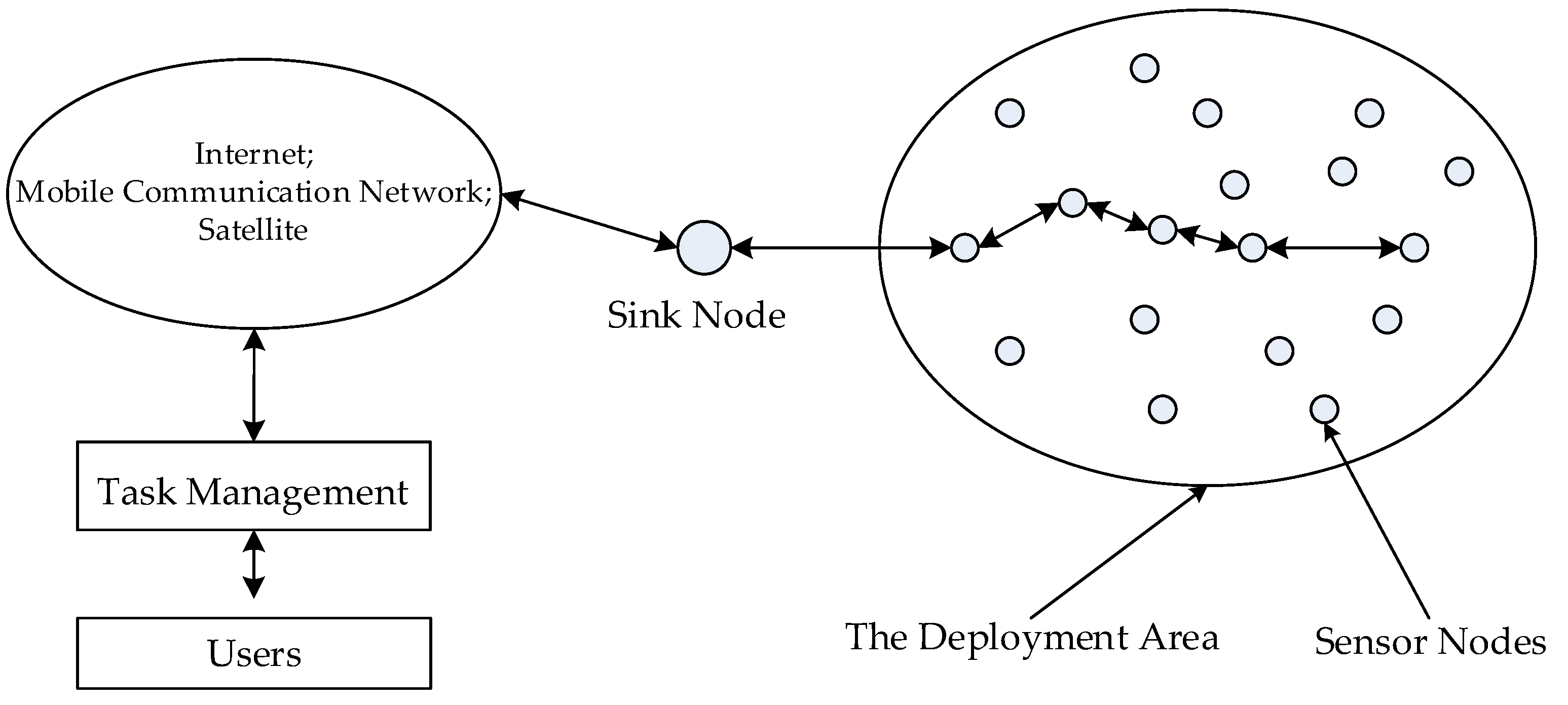
WSN is the core component of the Internet of Things. It has the advantages of large scale, low cost, strong adaptability and excellent expansibility, which makes the transmission, processing and application of information in an innovative way. With the development of communication technology, WSN has been widely used in national defense deployment, military reconnaissance, geological survey, intelligent agriculture and other fields, realizing the combination of the Internet of Things and the real world. The nodes in WSN can be divided into sink nodes and other nodes [1]. Generally, sink nodes has strong storage and communication capacity. It can be either an enhanced sensor node or a gateway device with a communication interface. The main task of the sink node is to conduct data interaction with the outside world through a variety of ways, and connect WSN with some other external networks (such as Internet, satellite, 4G/5G communication network and so on) [2]. The main task of other nodes is to collect data in the environment and send the data to the sink node, and then sink node will feedback the data to terminal computer or users [3]. A typical WSN structure is shown in Figure 1.

However, in most cases, the data collected by the sensor nodes must be combined with the location of the sensor nodes to be meaningful. Even more, sometimes users just need the sensor nodes to send back its own location. Therefore, the location of sensor nodes is an important part of WSN, and how to make the location calculation of sensor nodes closer to the reality has become the focus of research in the field of WSN.

1.2. Research Status

At present, sensor nodes localization method can be roughly classified into three categories: the range-based localization method based on external device, the range-free localization method based on network topology structure, the intelligent optimization algorithm localization method. The range-based localization method needed additional distance measurement equipment in the sensor nodes, which would increase the extra hardware costs. And in the forests, swamps, volcanoes and other special circumstances, the precision of distance measuring instrument is easily influenced by adverse environment conditions, which will cause the whole network to paralysis. Therefore, in the case of limited resources and environmental conditions, the range-based localization method is not applicable. For the intelligent optimization algorithm localization method, it usually obtains the coordinates of sensor nodes through thousands of iterations. However, excessive iterative calculation will consume a large amount of energy, which will undoubtedly shorten the life of sensor nodes. In addition, the experiment proves that the localization effect of the intelligent optimization algorithm is very poor in some cases, which is mainly because the intelligent optimization algorithm cannot search further when the coordinates of the beacon nodes is extremely lacking [4]. Therefore, the localization method based on intelligent optimization algorithm is not suitable for WSN. Compared with the above two localization methods, the range-free localization method does not need additional ranging equipment and a lot of calculation. Only according to the network architecture and the connectivity between sensor nodes the coordinates of unknown nodes can be estimated, which can meet the requirements of WSN on energy consumption, cost, application environment and other conditions. To sum up, the range-free localization method is the focus of current research.

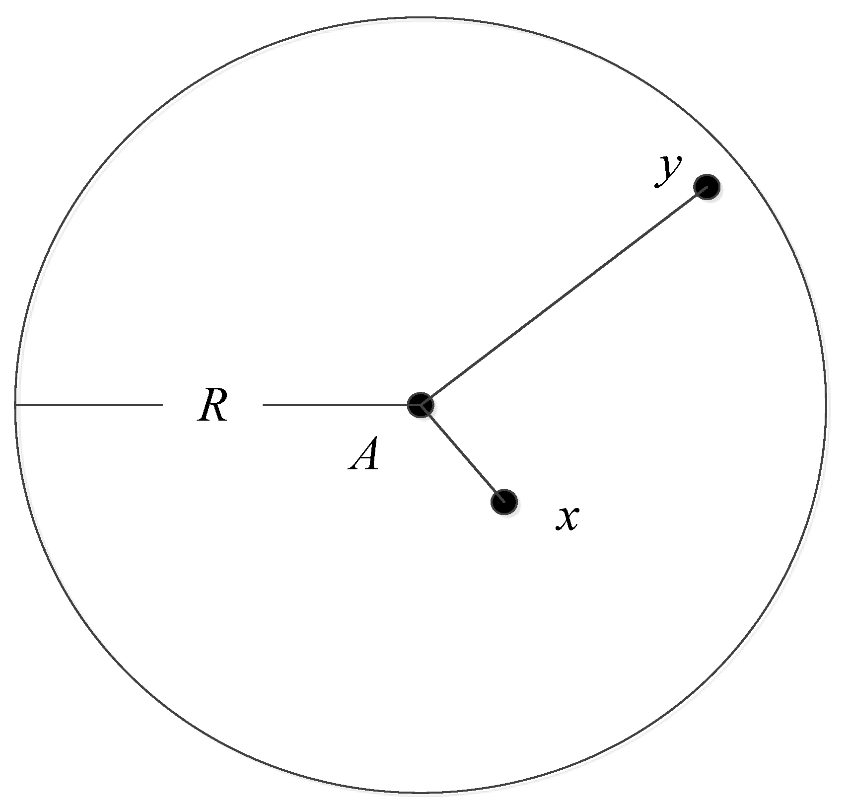
DV-Hop algorithm is the most concerned range-free localization algorithm by researchers at present, and it has the advantages of low complexity and good scalability. In DV-Hop algorithm, hop error is the main reason for the unsatisfactory localization accuracy. As shown in Figure 2, the unknown nodes $x$ and $y$ are both located in the communication circle of beacon node $A$, and $Ax\ll Ay$. However, according to DV-Hop, $Ax=Ay$ is obtained. So the result of the one hop distance is seriously inconsistent with the actual situation. Therefore, the traditional DV-Hop algorithm will cause a large distance estimation error and greatly reduce the accuracy of the final localization results. Aiming at this problem, the relevant literature at home and abroad has given the corresponding solution strategy. In Reference [5], Shi D et al. adopted the minimization of average hop error to correct the location of unknown nodes, which has optimized the localization accuracy. In Reference [6], Xue D put forward a genetic optimization DV-Hop localization algorithm. This algorithm was improved by error distance weighting, and the location of unknown nodes was obtained by using the weighted method and analyzing the distribution of beacon nodes, which had lower localization error than DV-Hop. Shi Q proposed a distance weighted algorithm based on DV-Hop in Reference [7],which determined the weight value of least squares by taking advantage of the different influence of beacon nodes, then used the weighted likelihood estimation and trilateral measurement localization to complete localization, thus improving the localization accuracy. In Reference [8], Yi Shang proposed an improved MDS-MAP localization algorithm, which was designed to make MDS-MAP localization algorithm also suitable for distributed location calculation. Since the improved MDS-MAP algorithm divides the whole network into small areas, the MDS-MAP algorithm is implemented in local areas to improve the localization accuracy. Wu C and Yang T proposed an improved DV-Hop algorithm in [9], this algorithm put forward an improvement wireless channel model and a refinement method for the irregularity of WSN based on node degree, improved the poor performance of DV-Hop algorithm in localization accuracy. In Reference [10], Han F et al. proposed a WND-DV-Hop algorithm based on weighting factor. By correcting the counting of one hop between nodes, a weighting coefficient was constructed based on the number of hops, which reduced the influence of beacon nodes with large hops on the localization result. Error correction is carried out after the unknown nodes complete localization, which further improves the localization accuracy. In Reference [11], Li J et al. proposed a new heuristic algorithm based on DV-Hop, which named parallel compact cat swarm optimization (PCCSO). PCCSO algorithm has three communication methods, and the localization result is better than DV-Hop algorithm. Song L et al. proposed a DV-Hop localization algorithm based on the glowworm swarm optimisation (GSO) of mixed chaotic strategy (MGDV-Hop) in Reference [12]. In MGDV-Hop algorithm, the fitness function is established based on the GSO algorithm and through hundreds of iterations to complete the localization. MGDV-Hop algorithm reduces the average localization error to a certain extent.

In general, most of algorithms are optimized on the basis of DV-Hop algorithm, and it has improved the localization accuracy. However, these algorithms still use the distance calculation method of DV-Hop, which multiplies the number of hops by the single hop correction value, so it is still unable to fundamentally avoid the impact of the error caused by the hop distance and the number of hops on the localization results [13]. To solve this problem, this paper proposes a VP-DC localization algorithm. In the distance estimation stage, using the virtual partition algorithm and optimal path search algorithm to calculate the distance, the DV-Hop distance calculation method is abandoned, avoid the hop error effectively. A large number of experiments have proved that the VP-DC algorithm can improve the accuracy of distance estimation between nodes and greatly improve the localization accuracy. It has strong robustness and can be well applied to WSN.

2. VP-DC Localization Algorithm

For avoid the impact of hop error on localization results, this paper proposes a virtual partition algorithm to estimate each hop distance on the shortest communication path between unknown node and beacon node, then calculates the distance from beacon node to unknown node according to the distance estimation method based on the optimal path search and distance correction.

2.1. Virtual Partition Algorithm

If the communication radius of the node is $R$, then the communication area of the beacon node is divided into several concentric circles with $R/m,2R/m,\cdots \cdots R$ as the radiuses ($m$ is the number of concentric circles), and unknown nodes within the communication range of the beacon node construct virtual circle with $R/m$ as radius. Then, according to the geometric analysis, obtain the area equations of the parts where the virtual circle intersects with each of concentric circles. Finally, the distance of one hop is obtained according to the distribution of nodes in each intersecting parts satisfying the Poisson Distribution solution equation. Since the nodes are randomly distributed, the distance of one hop calculated by different intersecting parts may be different. Therefore, this paper weights these distances to further reduce error. When dividing concentric circles, the larger the value of $m$, the more the intersection parts between the concentric circles and the virtual circle, and the higher the accuracy of the distance calculated by weighting. However, when the distribution of nodes is sparse, leading to the intersection parts are too small and no nodes in some intersection parts, which does not satisfy the Poisson Distribution model, resulting in large distance estimation error. According to a large number of simulation data, when $m=3$, the nodes distribution in each intersection part is the closest to Poisson Distribution model, which can meet the characteristics of WSN node random distribution.

As shown in Figure 3, it is known that $B$ is a beacon node, $U_1,U_2,U_3\cdots U_i$ are unknown nodes, $R$ is communication radius. With $B$ as the center of the circle and $R/3$, $2R/3$, $R$ as the radius, the communication circle of the $B$ is divided into three concentric circles. The unknown nodes located inside the communication circle of $B$ are constructed as virtual circle with the radius of $R/3$. Taking the unknown node $U_i$ as an example, assuming that the distance from $U_i$ to $B$ is $d_i$, and the intersecting areas of the virtual circle of $U_i$ and the three concentric circles of beacon node $B$ are $S_{i1}$, $S_{i2}$, $S_{i3}$ respectively. By analyzing geometry, $S_{i1}$ can be expressed as:

$$\begin{array}{cc}\hfill S_{i1}=& R^{2}arccos\left[\frac{\left(d_{i1}^2+R^2+{\left(1/9R\right)}^2\right)}{2d_{i1}R}\right]+{\left(1/9R\right)}^{2}arccos\left[\left(d_{i1}^2+{\left(1/9R\right)}^2-R^2\right)/\left(2d_{i1}/9R\right)\right]\hfill \\ & \hspace{0.33em}-1/2\sqrt{4d_{i1}^2{\left(1/9R\right)}^2-{\left(d_{i1}^2-R^2+{\left(1/9R\right)}^2\right)}^2}\hfill \end{array}$$

(1)

$S_{i2}$ can be expressed as:

$$\begin{array}{cc}\hfill S_{i2}=& R^{2}arccos\left[\frac{\left(d_{i2}^2+R^2+{\left(1/3R\right)}^2\right)}{2d_{i2}R}\right]-S_{i1}+{\left(1/3R\right)}^{2}arccos\left[\left(d_{i2}^2+{\left(1/3R\right)}^2\right)-R^2/\left(2d_{i2}/3R\right)\right]\hfill \\ & \hspace{0.33em}-1/2\sqrt{4d_{i2}^2{\left(1/3R\right)}^2-{\left(d_{i2}^2-R^2+{\left(1/3R\right)}^2\right)}^2}\hfill \end{array}$$

(2)

$S_{i3}$ can be expressed as:

$$\begin{array}{cc}\hfill S_{i3}=& \pi R^2-R^{2}arccos\left[\frac{\left(d_{i3}^2+R^2+{\left(1/3R\right)}^2\right)}{2d_{i3}R}\right]+{\left(1/3R\right)}^{2}arccos\left[\left(d_{i3}^2+{\left(1/3R\right)}^2\right)-R^2/\left(2d_{i3}/3R\right)\right]\hfill \\ & -1/2\sqrt{4d_{i3}^2{\left(1/3R\right)}^2-{\left(d_{i3}^2-R^2+{\left(1/3R\right)}^2\right)}^2}\hfill \end{array}$$

(3)

$d_{i1}$, $d_{i2}$, $d_{i3}$ are the distances from $U_i$ to $B$ in these three cases respectively. The distribution of nodes in WSN is random, so the probability that the unknown node $U_i$ is located inside and outside the communication circle of beacon node $B$ approximately satisfies the Poisson Distribution model [14]. The probability function of Poisson Distribution model is:

$$P=\frac{{\left(\lambda D\right)}^k}{k!}{e}^{-\lambda D} \left(k=0, 1,\cdots \cdots n\right)$$

(4)

It is known that the area of the communication circle of $B$ is $\pi R^2$ and the quantity of nodes in the communication circle is $n_B$; the quantity of nodes in the virtual circle of unknown node $U_i$ is $n_i$; and the quantity of nodes in the three intersecting areas are $n_{i1}$, $n_{i2}$, $n_{i3}$ respectively. According to the Poisson distribution model, the following formulas can be listed:

$$S_{i1}\approx \pi R^2\times \frac{n_{i1}}{n_B}$$

(5)

$$S_{i2}\approx \pi R^2\times \frac{n_{i2}}{n_B}$$

(6)

$$S_{i3}\approx \pi R^2\times \frac{n_{i3}}{n_B}$$

(7)

By Equations (5)–(7) [15], the values of $S_{i1}$, $S_{i2}$, $S_{i3}$ can be obtained. Substitute the values of $S_{i1}$, $S_{i2}$, $S_{i3}$ into Equations (1)–(3), and then, by solving these three Equations, the values of the unknowns $d_{i1}$, $d_{i2}$, $d_{i3}$ can be obtained respectively. Finally, $d_{i1}$, $d_{i2}$, $d_{i3}$ are weighted and averaged to obtain $d_i$, which is can be expressed as:

$$d_i=d_{i1}\times \frac{n_{i1}}{n_i}+d_{i1}\times \frac{n_{i2}}{n_i}+d_{i1}\times \frac{n_{i3}}{n_i}$$

(8)

Thus, the distance of one hop on the communication path is obtained.

2.2. Distance Estimation Method Based on Optimal Path Search and Distance Correction

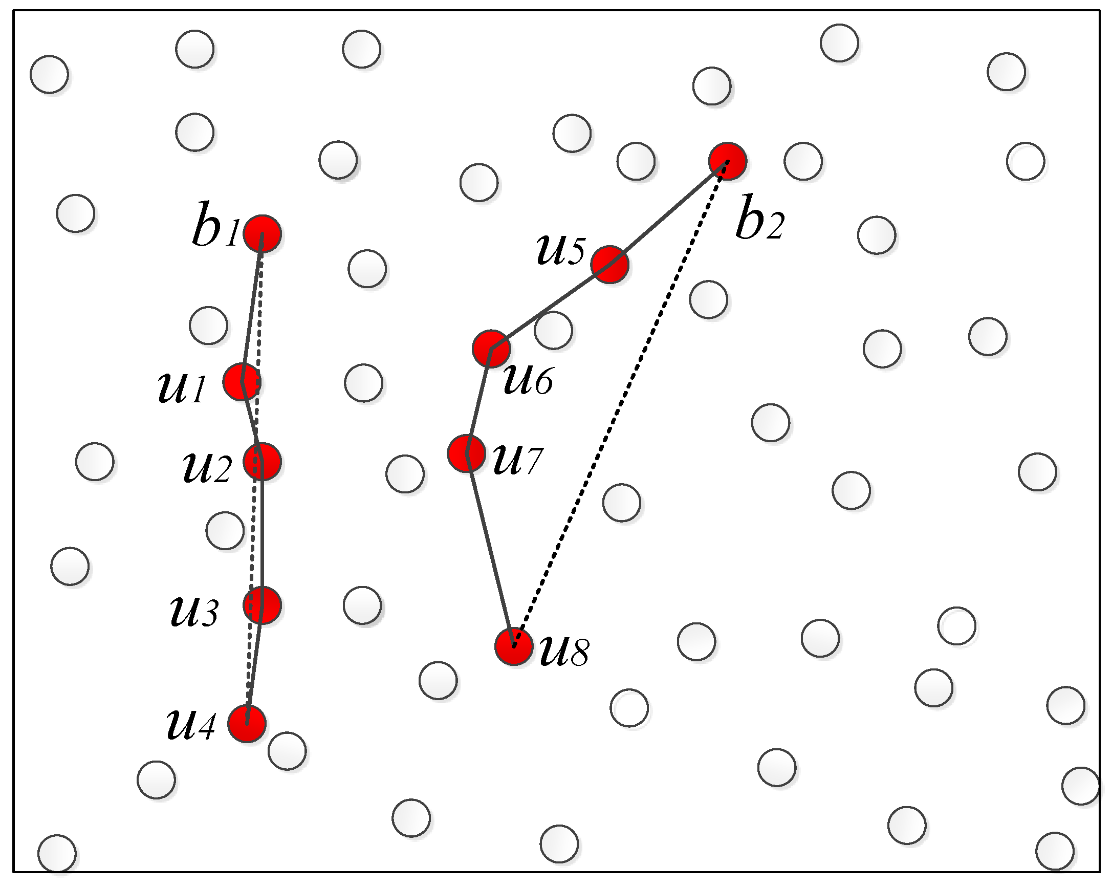
In the distance estimation stage, the length of the shortest communication path between nodes is regarded as the actual distance between nodes in the traditional localization algorithm. As shown in Figure 4, $u_1, u_2,\cdots u_8$ are unknown nodes; $b_1$, $b_2$ are beacon nodes. From the figure, it can be seen that the shortest communication path between $b_1$ and $u_4$ is similar to a straight line, so the shortest communication distance is approximately equal to the actual distance between $b_1$ and $u_4$, which is $d_{b_1{u}_1}+d_{u_1{u}_2}+d_{u_2{u}_3}+d_{u_3{u}_4}\approx d_{b_1{u}_4}$; However, the shortest communication distance between $b_2$ to $u_8$ obviously longer than the actual distance, namely the $d_{b_2{u}_5}+d_{u_5{u}_6}+d_{u_6{u}_7}+d_{u_7{u}_8}\gg d_{b_2{u}_8}$. To sum up, when the shortest communication path between nodes is tortuous or deviates from a straight line, the shortest communication distance is far longer than the real distance between nodes [16]. In this case, if the shortest communication distance is still taken as the actual distance between nodes, it will bring a large distance estimation error and eventually reduce the accuracy of localization results. For avoid the distance estimation error mentioned above, this paper proposes a distance estimation method based on optimal path search and distance correction.

2.2.1. Optimal Path Search Algorithm

The aim of the optimal path search algorithm is to find the shortest communication path between a pair of beacon nodes in the whole network, which is most similar to the shortest communication path from the unknown node to the beacon node. This shortest communication path between the pair of beacon nodes is the beacon path of the shortest communication path from the unknown node to the beacon node. The Ochiai coefficient can indicate the similarity of two sets. The more same elements in the two sets, the higher the similarity between the two sets. In this algorithm, Ochiai coefficient [17] is used to represent the similarity degree between the shortest communication path and its beacon path. Take the nodes passed on the communication path into set, the more identical nodes on the two paths, the larger the Ochiai coefficient is, the higher the similarity between the two communication paths is, and vice versa. If the set composed of nodes on the communication path between beacon node pair is $A$, the set composed of nodes on the shortest communication path from the unknown node to the beacon node is $B$, the number of nodes in set $A$, $B$ is respectively $N\left(A\right)$, $N\left(B\right)$, the Ochiai coefficient can be defined as:

$$chiai\left(A,B\right)=\frac{N\left(A\cap B\right)}{\sqrt{N\left(A\right)\times N\left(B\right)}}$$

(9)

The detailed steps of the optimal path search algorithm are as follows:

• Traverse all the combination of beacon node pairs in the WSN, the set composed of nodes on the shortest communication path between each beacon node pair is respectively expressed as: $A_1,A_2\cdots \cdots A_k\cdots \cdots A_n$.
• The set composed of nodes on the shortest communication path between $u_i$ and $b_j$ is recorded as $B$.
• Calculate the Ochiai coefficients of $B$ and $A_1,A_2\cdots \cdots A_k\cdots \cdots A_n$ respectively, and find the beacon node pair corresponding to the maximum value of Ochiai. Then take the shortest communication path between this beacon node pair as the beacon path of the shortest communication path between $u_i$ and $b_j$.

2.2.2. Distance Correction

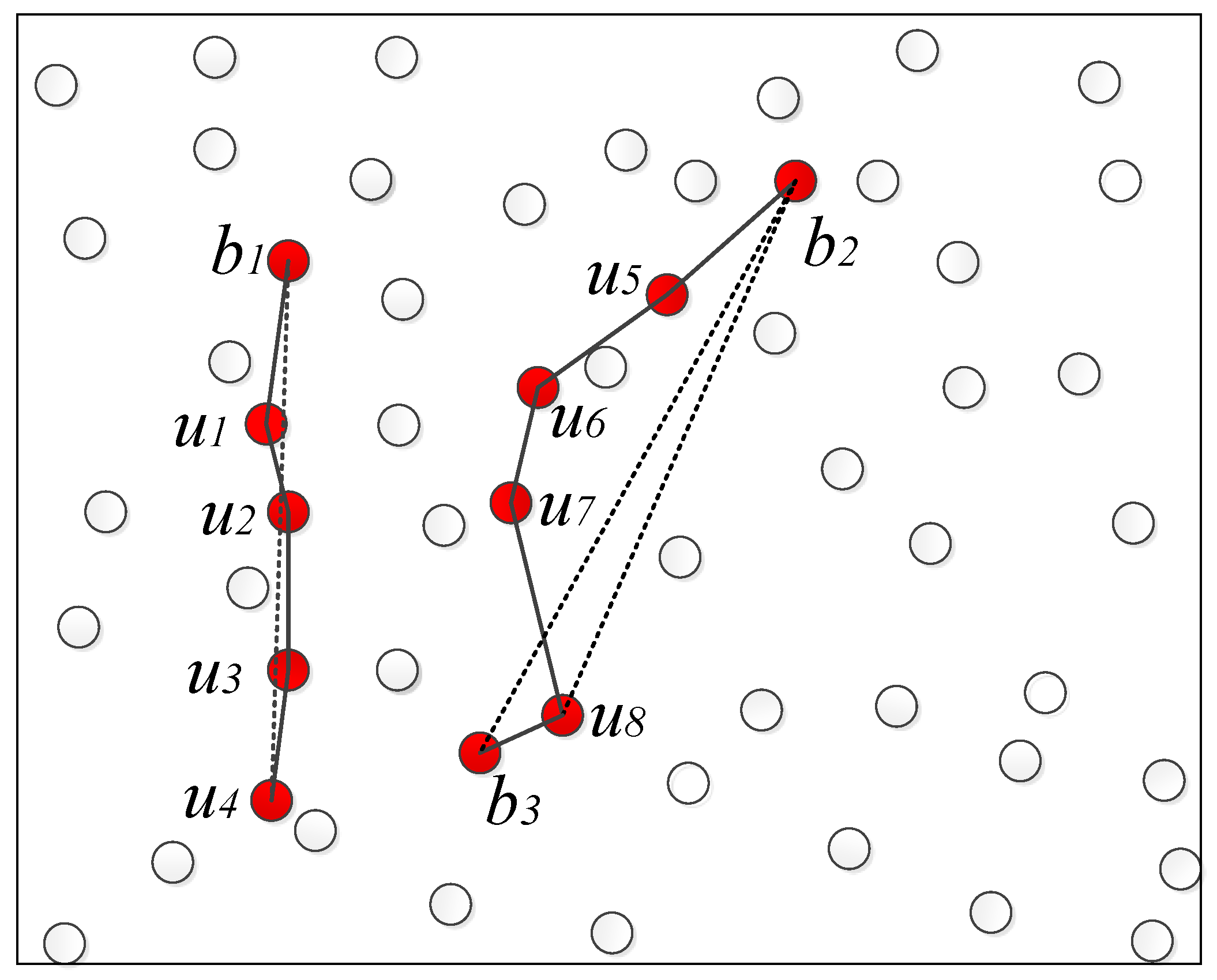
When the shortest communication path between nodes is tortuous or deviates from a straight line, the shortest communication distance is far longer than the real distance between nodes. Therefore, this paper corrects the length of the shortest communication path based on the Ochiai coefficient of the shortest communication path and its beacon path and the length of the beacon path to further reduce the distance estimation error. For example, in Figure 5, $b_1$, $b_2$, $b_3$ are beacon nodes, $u_1,u_2,\cdots u_8$ are unknown nodes, and the distance between $u_8$ and $b_2$ is unknown. The specific steps of the distance estimation between $u_8$ and $b_2$ based on optimal path search and distance correction are as follows:

• Firstly, the distance of one hop between nodes can be obtained according to the virtual partition algorithm. Then, the length of the shortest communication path could be calculated by summing the distance of each hop. Therefore, the length of the shortest communication path between $u_8$ and $b_2$ is:

  $$l_{u_8{b}_2}=d_{b_2{u}_5}+d_{u_5{u}_6}+d_{u_6{u}_7}+d_{u_7{u}_8}$$

  (10)
• The optimal path search algorithm is implemented to find the beacon path of the shortest communication path from $u_8$ to $b_2$. By calculating the Ochiai coefficient, it is found that the shortest communication path between $b_2$ and $b_3$ is most similar to that between $u_8$ and $b_2$. Therefore, the shortest communication path between $b_2$ and $b_3$ is the beacon path. According to the virtual partition algorithm, the length of beacon path is:

  $$l_{b_2{b}_3}=d_{b_2{u}_5}+d_{u_5{u}_6}+d_{u_6{u}_7}+d_{u_7{u}_8}+d_{u_8{b}_3}$$

  (11)

  If the coordinates of beacon nodes $b_2$, $b_3$ respectively: $\left(x_{b_2},y_{b_2}\right)$, $\left(x_{b_3},y_{b_3}\right)$, then the distance between $b_2$ to $b_3$ is:

  $$d_{b_2{b}_3}=\sqrt{{\left(x_{b_2}-x_{b_3}\right)}^2+{\left(y_{b_2}-y_{b_3}\right)}^2}$$

  (12)
• If the similarity coefficient between the shortest communication path and the beacon path is $ochia{i}_{u_8{b}_2}$, then the formula for the distance from $u_8$ to $b_2$ is:

  $$d_{u_8{b}_2}=\left[l_{u_8{b}_2}\times \left(1-ochia{i}_{u_8{b}_2}\right)\right]+\left[l_{u_8{b}_2}\times ochia{i}_{u_8{b}_2}\times \frac{d_{b_2{b}_3}}{l_{b_2{b}_3}}\right]$$

  (13)

  To sum up, the formula for the distance from $u_i$ to $b_j$ is:

  $$d_{u_i{b}_j}=\left[l_{u_i{b}_j}\times \left(1-ochia{i}_{u_i{b}_j}\right)\right]+\left[l_{u_i{b}_j}\times ochia{i}_{u_i{b}_j}\times \frac{d_{b_m{b}_n}}{l_{b_m{b}_n}}\right]$$

  (14)

  In Equation (14), $l_{u_i{b}_j}$ is the length of the shortest communication path from $u_i$ to $b_j$. $l_{b_m{b}_n}$ is the length of the beacon path; $d_{b_m{b}_n}$ is the actual distance between the beacon nodes at both ends of the beacon path; $ochia{i}_{u_i{b}_j}$ is the similarity coefficient between the shortest communication path from $u_i$ to $b_j$ and its beacon path.

2.3. Coordinate Calculation of Unknown Nodes

Assume that the quantity of beacon nodes in the entire network is $n$, the coordinates of these beacon nodes are: $b_1\left(x_{b_1},y_{b_1}\right)\cdots \cdots b_j\left(x_{b_j},x_{b_j}\right)\cdots \cdots b_n\left(x_{b_n},y_{b_n}\right)$. According to the optimal path search and distance correction, the distances between $u_i$ and each beacon node can be obtained. The distances between $u_i$ and each beacon node are: $d_{u_i{b}_1}\cdots \cdots d_{u_i{b}_j}\cdots \cdots d_{u_i{b}_n}$, so the follwing equations can be obtained:

$$\{\begin{array}{c}{\left(x_{b_1}-x_{u_i}\right)}^2+{\left(y_{b_1}-y_{u_i}\right)}^2=d_{u_i{b}_1}^2\\ ⋮\\ {\left(x_{b_j}-x_{u_i}\right)}^2+{\left(y_{b_j}-y_{u_i}\right)}^2=d_{u_i{b}_j}^2\\ ⋮\\ {\left(x_{b_n}-x_{u_i}\right)}^2+{\left(y_{b_n}-y_{u_i}\right)}^2=d_{u_i{b}_n}^2\end{array}$$

(15)

According to the trilateral measurement:

$$\{\begin{array}{c}{x}_{b_1}^2-x_{b_n}^2-2x_{u_i}(x_{b_1}-x_{b_n})+y_{b_1}^2-y_{b_n}^2-2y_{u_i}(y_{b_1}-y_{b_n})=d_{u_i{b}_1}^2-d_{u_i{b}_n}^2\\ ⋮\\ x_{b_j}^2-x_{b_n}^2-2x_{u_i}(x_{b_j}-x_{b_n})+y_{b_j}^2-y_{b_n}^2-2y_{u_i}(y_{b_j}-y_{b_n})=d_{u_i{b}_j}^2-d_{u_i{b}_n}^2\\ ⋮\\ x_{b_{n-1}}^2-x_{b_n}^2-2x_{u_i}(x_{b_{n-1}}-x_{b_n})+y_{b_{n-1}}^2-y_{b_n}^2-2y_{u_i}(y_{b_{n-1}}-y_{b_n})=d_{u_i{b}_{n-1}}^2-d_{u_i{b}_n}^2\end{array}$$

(16)

Express the Equation set (16) in the form of $DX=E$, so:

$$E=\left[\begin{array}{c}{x}_{b_1}^2-x_{b_n}^2+y_{b_1}^2-y_{b_n}^2+d_{u_i{b}_n}^2-d_{u_i{b}_1}^2\\ ⋮\\ x_{b_j}^2-x_{b_n}^2+y_{b_j}^2-y_{b_n}^2+d_{u_i{b}_n}^2-d_{u_i{b}_j}^2\\ ⋮\\ x_{b_{n-1}}^2-x_{b_n}^2+y_{b_{n-1}}^2-y_{b_n}^2+d_{u_i{b}_n}^2-d_{u_i{b}_{n-1}}^2\end{array}\right]$$

(17)

$$D=\left[\begin{array}{cc}2\left(x_{b_{n-1}}-x_{b_n}\right)& 2\left(y_{b_1}-y_{b_n}\right)\\ ⋮& ⋮\\ 2\left(x_{b_j}-x_{b_n}\right)& 2\left(y_{b_j}-y_{b_n}\right)\\ ⋮& ⋮\\ 2\left(x_{b_{n-1}}-x_{b_n}\right)& 2\left(y_{b_{n-1}}-y_{b_n}\right)\end{array}\right]$$

(18)

According to the least square method:

$$\mathrm{X}={\left(D^{T}D\right)}^{-1}{D}^{T}E$$

(19)

$$X=\left[\begin{array}{c}{x}_{u_i}\\ y_{u_i}\end{array}\right]$$

(20)

Therefore, the coordinate of the unknown node $u_i$ is $\left(x_{u_i},y_{u_i}\right)$.

3. Simulation Experiment and Analysis

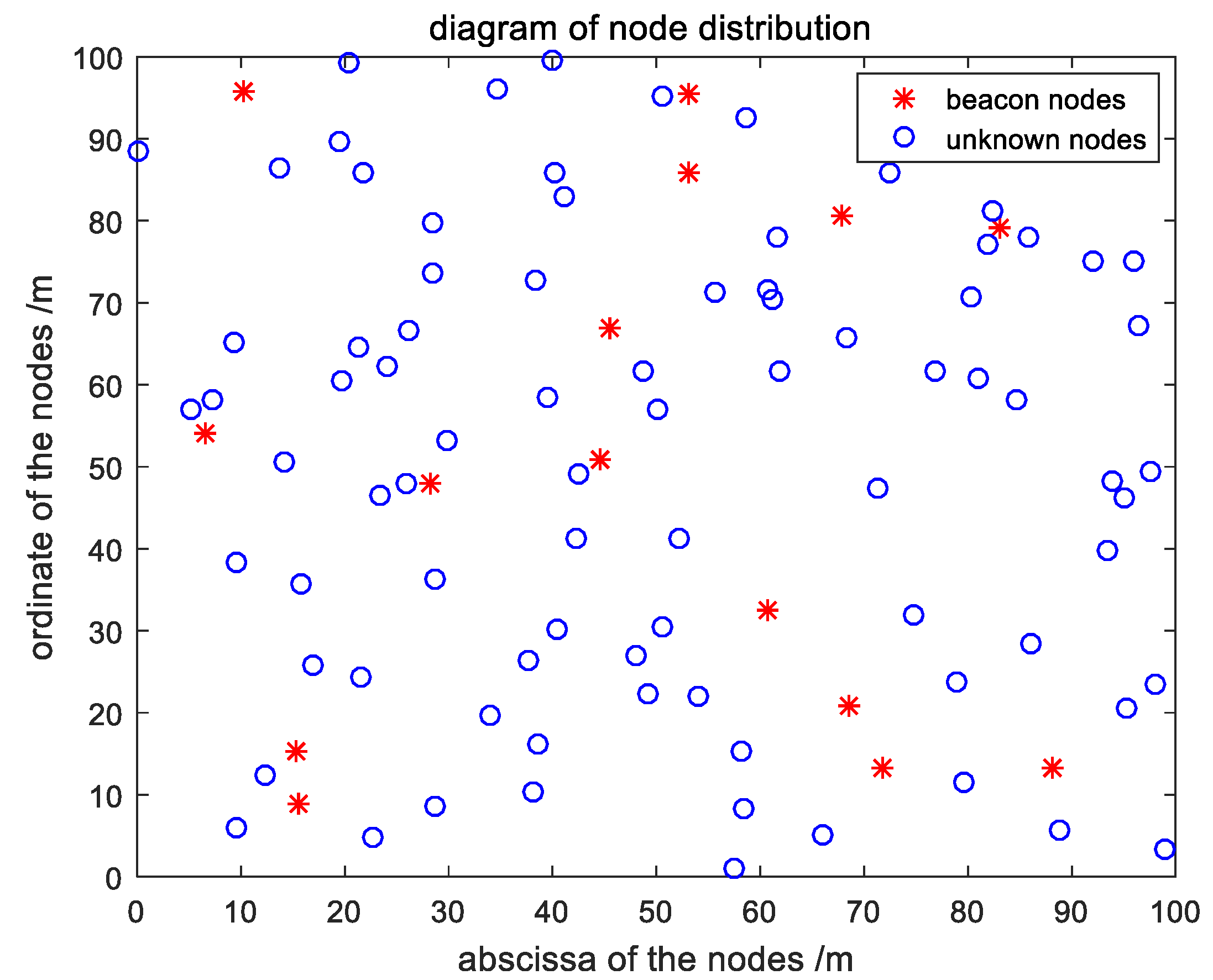
In order to test the performance of the VP-DC algorithm, Windows 7 operating system and MATLAB 2016a simulation software were used for experiments. Firstly, randomly deploy 100 nodes in the 100 m × 100 m region. Then the simulations are carried out with different quantity of beacon nodes and communication radius. Finally, according to the experimental results, compare VP-DC localization algorithm with MGDV-Hop, DV-Hop and WND-DV-Hop localization algorithms. Figure 6 shows the distribution of nodes when the quantity of beacon nodes in the network is 15. The formula of average localization error in this paper is:

$$ErrorMean=\frac{1}{T}{\displaystyle \sum }_{i=1}^n\frac{{{\displaystyle \sum }}_{i=1}^n\sqrt{{\left(x_{u_i}^{\prime }-x_{u_i}\right)}^2+{\left(y_{u_i}^{\prime }-y_{u_i}\right)}^2}}{n}$$

(21)

In Equation (21), $T$ is the times of experiments performed, $n$ is the number of unknown nodes, $\left(x_{u_i}^{\prime },y_{u_i}^{\prime }\right)$ is the actual coordinate of unknown node $u_i$, and $\left(x_{u_i},y_{u_i}\right)$ is the estimated coordinate of $u_i$.

3.1. Influence of the Number of Beacon Nodes on the Average Localization Error and Algorithm Operation Time

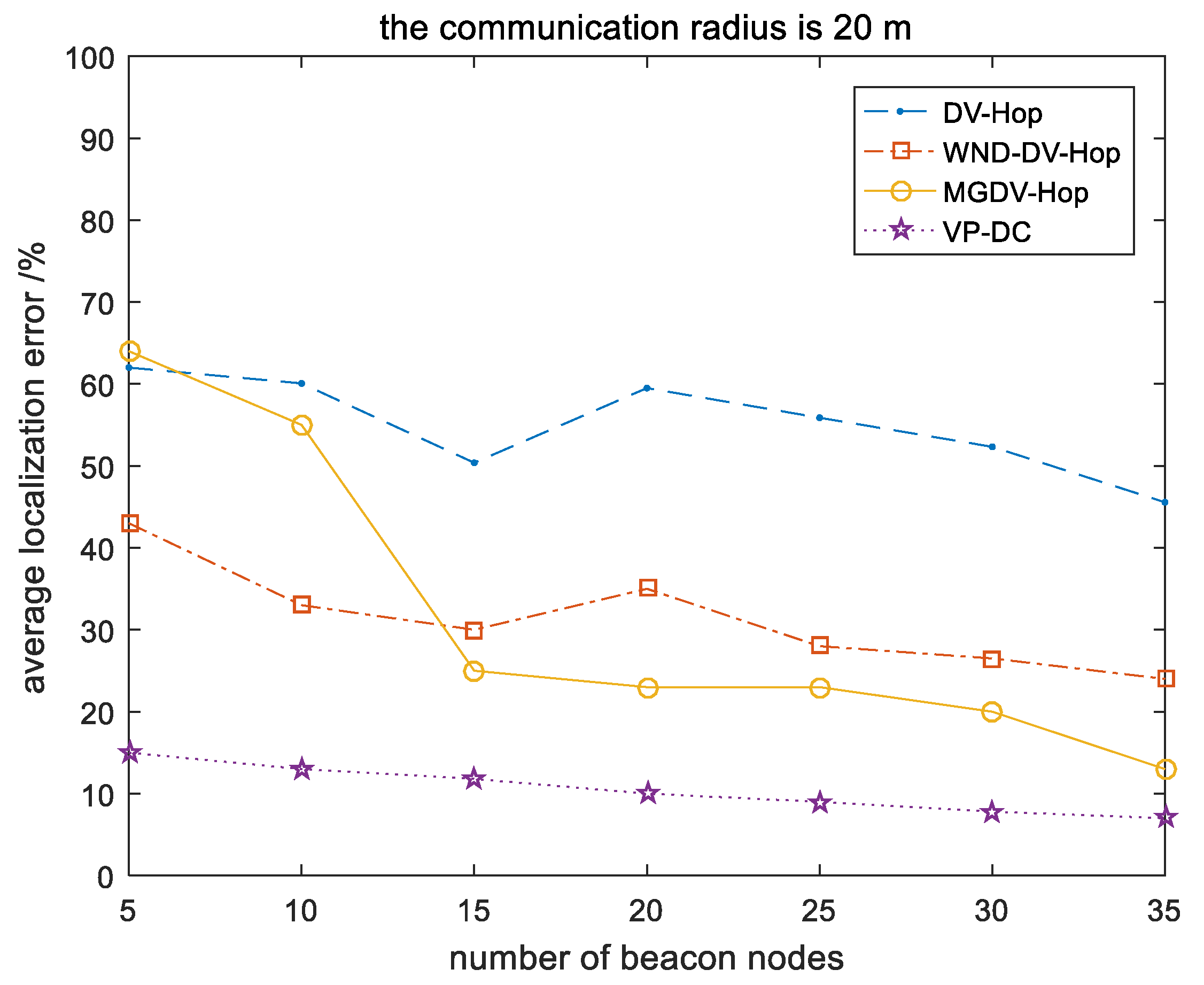
When the communication radius is 20 m, VP-DC and the other three algorithms are simulated with different number of beacon nodes, and evaluate each algorithm on the basis of the simulation results.

• The influence of the number of beacon nodes on the localization accuracy of each algorithm is shown in Figure 7. Figure 7 shows that due to the accumulation of hop error, the simulation result of DV-Hop algorithm is worse than other localization algorithms. When the distribution of beacon nodes is extremely sparse, the localization error of MGDV-Hop algorithm is very large. This is because the glowworm swarm optimisation algorithm cannot search further when the beacon node coordinates are extremely lacking. In general, the localization results of VP-DC algorithm are least affected by the quantity of beacon nodes, and the localization accuracy is significantly higher than other three algorithms.
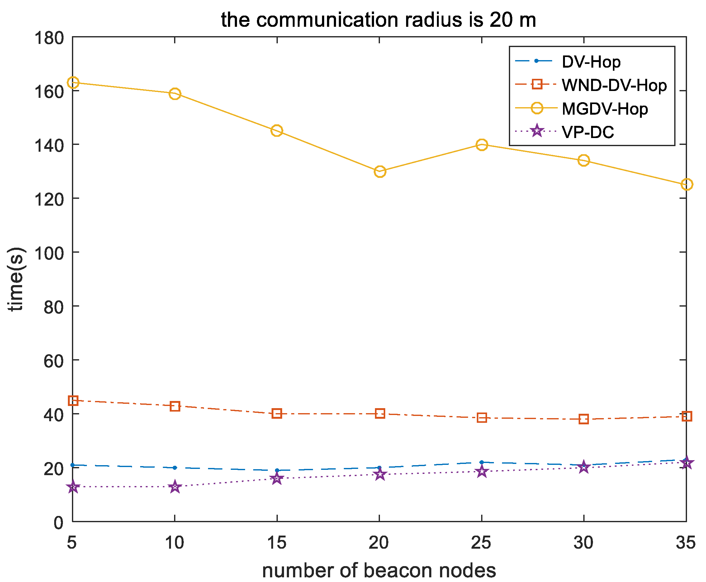
• The influence of the number of beacon nodes on the operation time of each localization algorithm is shown in Figure 8. The MGDV-Hop algorithm which based on GSO algorithm needs hundreds of iterations to complete localization [18], so it takes the longest time. The Figure 8 shows that the operation time of DV-Hop algorithm and WND-DV-Hop algorithm is very steady. As the quantity of beacon nodes increases, the traversal process of the optimal path search algorithm takes longer time, so, the operation time of VP-DC algorithm tends to increase slightly. However, VP-DC algorithm has the shortest operation time and the least amount of calculation, so the energy consumption required for localization is also the least.

3.2. Influence of Nodes Communication Radius on Average Localization Error and Algorithm Operation Time

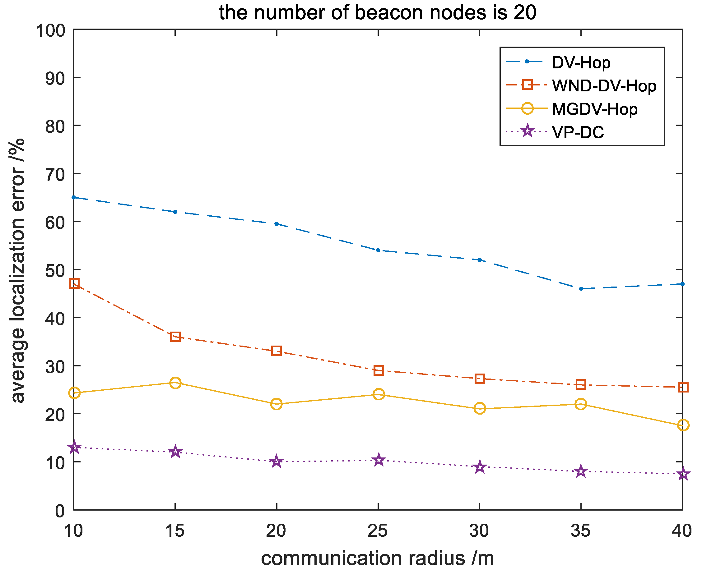
When number of beacon nodes is 20, simulate the VP-DC algorithm and the other three localization algorithms by constantly changing the communication radius. And evaluate each algorithm on the basis of the simulation results.

• The influence of the communication radius on the average localization error is shown in Figure 9. In Figure 9, the smaller the communication radius is, the worse the localization effect of DV-Hop algorithm and WND-DV-Hop algorithm. This is because the reduction of the communication radius will increase the number of hops on the shortest communication path, resulting in the accumulation of hop error, and ultimately reduce the localization accuracy [19]. The distance estimation method of MGDV-Hop algorithm and VP-DC algorithm are irrelevant to the number of hops between nodes, so the localization accuracy is not affected by the communication radius. In general, the VP-DC algorithm has higher localization accuracy and better stability than the other three algorithms.
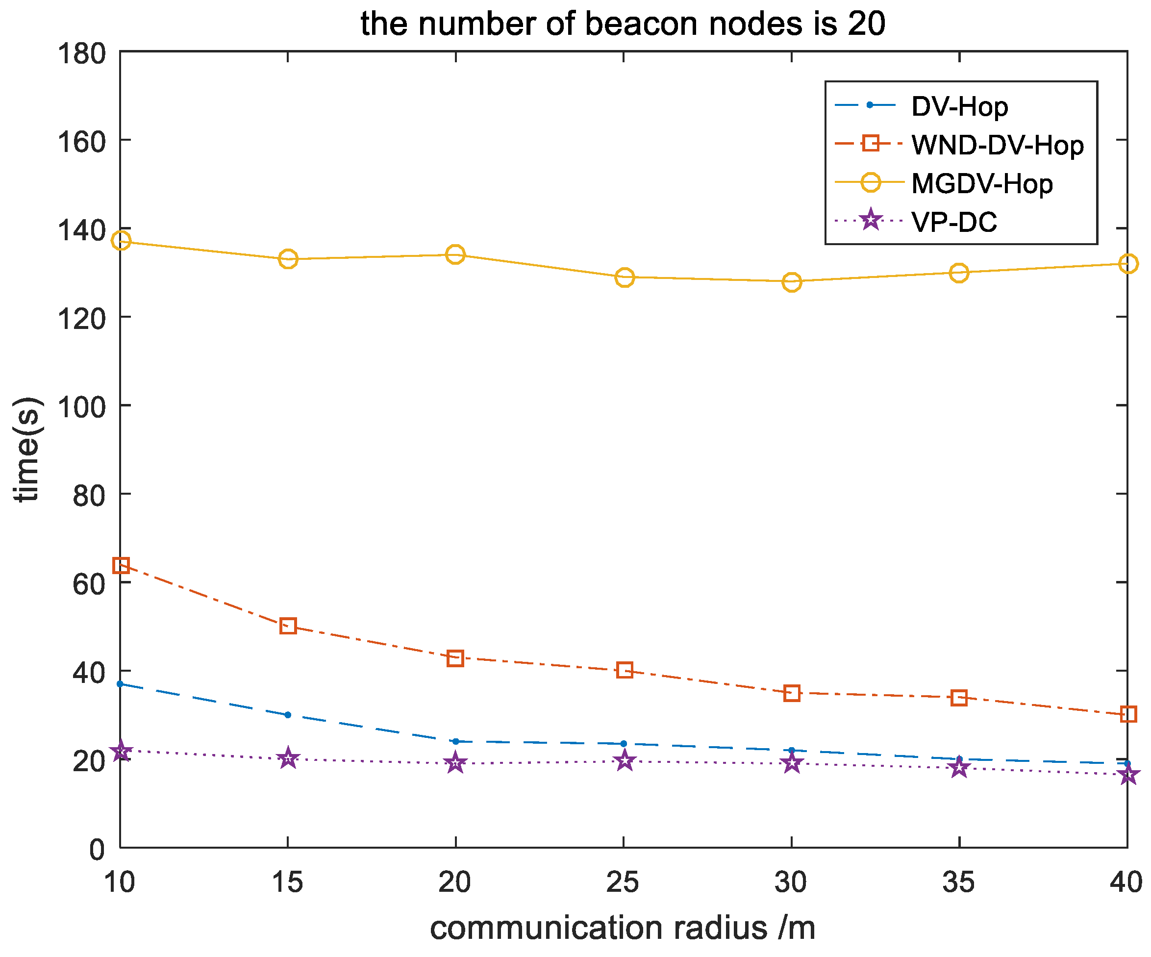
• The influence of nodes communication radius on algorithm operation time is shown in Figure 10. As shown in Figure 10, the operation time of MGDV-Hop is not affected by the communication radius, but it operation time is too long, which will cause large energy consumption. The operation time of DV-Hop algorithm and WND-DV-Hop algorithm decreases with the increase of communication radius, this is because the quantity of hops between nodes decreases with the increase of the communication radius, which reduces the calculation amount in the distance estimation stage. Compared with the other three algorithms, the operation time of VP-DC algorithm is very steady, and the operation time is the shortest.

4. Conclusions

This paper proposes a localization algorithm based on virtual partition and distance correction to solve the problems of hop error accumulation and low localization accuracy in nodes localization process. VP-DC algorithm estimates the distance according to virtual partition and optimal path search. Firstly, the distance of each hop between nodes is calculated according to the virtual partition algorithm, and the distance of each hop is summed to get the length of the shortest communication path between nodes. Then, find the beacon path of the shortest communication path based on the optimal path search algorithm. Finally, the unknown distance from unknown node to beacon node is obtained according to the beacon path and the distance correction formula. VP-DC localization algorithm abandons the traditional distance estimation method, avoiding the hop error accumulation, and greatly improves the localization accuracy of nodes. Through a large number of simulation tests, it is proved that the VP-DC algorithm has the characteristics of strong stability, high localization accuracy and short operation time, which could greatly improve the localization efficiency and prolong the service life of nodes. In the future research, the application of machine learning in node localization of WSN will be the focus of study.

References

- Thomson, C.; Wadhaj, I. Towards an energy balancing solution for wireless sensor network with mobile sink node. Comput. Commun. 2021, 170, 50–64. [Google Scholar] [CrossRef]
- Deng, Z.; Tang, S. A Novel Location Source Optimization Algorithm for Low Anchor Node Density Wireless Sensor Networks. Sensors 2021, 21, 1890. [Google Scholar] [CrossRef] [PubMed]
- Hao, Z.; Dang, J. A node localization algorithm based on Voronoi diagram and support vector machine for wireless sensor networks. Int. J. Distrib. Sens. Netw. 2021, 17, 1550147721993410. [Google Scholar] [CrossRef]
- Jiang, B. Research on wireless sensor location technology for biologic signal measuring based on intelligent bionic algorithm. Peer Peer Netw. Appl. 2020, 14, 2495–2500. [Google Scholar] [CrossRef]
- Shi, D.; Zhang, X. A Security Localization Algorithm Based on DV-Hop against Sybil Attack in Wireless Sensor Networks. J. Electr. Eng. Technol. 2020, 15, 919–926. [Google Scholar]
- Xue, D. Research of localization algorithm for wireless sensor network based on DV-Hop. EURASIP J. Wirel. Commun. Netw. 2019, 2019, 1–8. [Google Scholar] [CrossRef] [Green Version]
- Shi, Q.; Wu, C.; Zhang, J. Optimization for DV-Hop type of localization scheme in wireless sensor networks. J. Supercomput. 2021, 2021, 1–24. [Google Scholar]
- Shang, Y.; Ruml, W.; Zhang, Y. Localization from connectivity in sensor networks. IEEE Tracsactions Parallel Distrib. Syst. 2004, 15, 961–974. [Google Scholar] [CrossRef] [Green Version]
- Wu, C.; Yang, T. An improved DV-HOP algorithm was applied for the farmland wireless sensor network. J. Inf. Hiding Multimed. Signal Process. 2017, 8, 148–155. [Google Scholar]
- Han, F.; Izzeldin, I. An Enhanced Distance Vector-Hop Algorithm using New Weighted Location Method for Wireless Sensor Networks. Int. J. Adv. Comput. Sci. Appl. (IJACSA) 2020, 11, 0110563. [Google Scholar] [CrossRef]
- Li, J.; Gao, M. A parallel compact cat swarm optimization and its application in DV-Hop node localization for wireless sensor network. Wirel. Netw. 2021, 27, 2081–2101. [Google Scholar] [CrossRef]
- Song, L.; Zhao, L.; Ye, J. A DV-Hop positioning algorithm based on the glowworm swarm optimisation of mixed chaotic strategy. Int. J. Secur. Netw. 2019, 14, 23–33. [Google Scholar] [CrossRef]
- Kim, J.; Lee, D.; Hwang, J. Wireless Sensor Network (WSN) Configuration Method to Increase Node Energy Efficiency through Clustering and Location Information. Symmetry 2021, 13, 390. [Google Scholar] [CrossRef]
- Lee, W.S.; Kim, N.G. Omnidirectional Distance Estimation using ultrasonic in Wireless Sensor Networks. J. Inst. Internet Broadcasting Commun. 2009, 9, 85–91. [Google Scholar]
- Yasuyuki, H.; Tatsuya, K. Bayesian predictive distribution for a Poisson model with a parametric restriction. Commun. Stat.-Theory Methods 2020, 49, 3257–3266. [Google Scholar]
- Kotiyal, V.; Singh, A. ECS-NL: An Enhanced Cuckoo Search Algorithm for Node Localization in Wireless Sensor Networks. Sensors 2021, 21, 3576. [Google Scholar] [CrossRef] [PubMed]
- Zhou, Q.; Leydesdorff, L. The Normalization of Occurrence and Co-Occurrence Matrices in Bibliometrics Using Cosine Similarities and Ochiai Coefficients. J. Assoc. Inf. Sci. Technol. 2016, 67, 2805–2814. [Google Scholar] [CrossRef] [Green Version]
- Houriya, H.; Mohsen, J.; Saeedreza, S. Correction to: Improving lifetime of wireless sensor networks based on nodes’ distribution using Gaussian mixture model in multi-mobile sink approach. Telecommun. Syst. 2021, 77, 255–268. [Google Scholar]
- Qi, N.; Yin, Y. Comprehensive optimized hybrid energy storage system for long-life solar-powered wireless sensor network nodes. Appl. Energy 2021, 290, 116780. [Google Scholar] [CrossRef]
Figure 1.
Wireless sensor network structure diagram.
Figure 2.
Diagram of hop error.
Figure 3.
Diagram of virtual partition algorithm.
Figure 4.
Comparison diagram of the shortest communication distance and actual distance.
Figure 5.
Diagram for distance estimation.
Figure 6.
Diagram of random distribution of nodes.
Figure 7.
Relationship between the number of beacon nodes and the average localization error.
Figure 8.
Relationship between the number of beacon nodes and the operation time of the algorithm.
Figure 9.
Relationship between nodes communication radius and average localization error.
Figure 10.
Relationship between nodes communication radius and algorithm operation time.
Publisher’s Note: MDPI stays neutral with regard to jurisdictional claims in published maps and institutional affiliations. |
© 2021 by the authors. Licensee MDPI, Basel, Switzerland. This article is an open access article distributed under the terms and conditions of the Creative Commons Attribution (CC BY) license (https://creativecommons.org/licenses/by/4.0/).
Share and Cite
MDPI and ACS Style
Meng, Y.; Zhi, Q.; Dong, M.; Zhang, W. A Node Localization Algorithm for Wireless Sensor Networks Based on Virtual Partition and Distance Correction. Information 2021, 12, 330. https://0-doi-org.brum.beds.ac.uk/10.3390/info12080330
AMA Style
Meng Y, Zhi Q, Dong M, Zhang W. A Node Localization Algorithm for Wireless Sensor Networks Based on Virtual Partition and Distance Correction. Information. 2021; 12(8):330. https://0-doi-org.brum.beds.ac.uk/10.3390/info12080330
Chicago/Turabian StyleMeng, Yinghui, Qianying Zhi, Minghao Dong, and Weiwei Zhang. 2021. "A Node Localization Algorithm for Wireless Sensor Networks Based on Virtual Partition and Distance Correction" Information 12, no. 8: 330. https://0-doi-org.brum.beds.ac.uk/10.3390/info12080330
Note that from the first issue of 2016, this journal uses article numbers instead of page numbers. See further details here.