
Geometric Regularization of Local Activations for Knowledge Transfer in Convolutional Neural Networks

1
Department of Physics, University of Patras, 26504 Rion, Greece
2
Department of Computer Engineering & Informatics, University of Patras, 26504 Rion, Greece
*
Author to whom correspondence should be addressed.
Information 2021, 12(8), 333; https://0-doi-org.brum.beds.ac.uk/10.3390/info12080333
Submission received: 26 July 2021
/
Revised: 14 August 2021
/
Accepted: 17 August 2021
/
Published: 19 August 2021
Abstract
:In this work, we propose a mechanism for knowledge transfer between Convolutional Neural Networks via the geometric regularization of local features produced by the activations of convolutional layers. We formulate appropriate loss functions, driving a “student” model to adapt such that its local features exhibit similar geometrical characteristics to those of an “instructor” model, at corresponding layers. The investigated functions, inspired by manifold-to-manifold distance measures, are designed to compare the neighboring information inside the feature space of the involved activations without any restrictions in the features’ dimensionality, thus enabling knowledge transfer between different architectures. Experimental evidence demonstrates that the proposed technique is effective in different settings, including knowledge-transfer to smaller models, transfer between different deep architectures and harnessing knowledge from external data, producing models with increased accuracy compared to a typical training. Furthermore, results indicate that the presented method can work synergistically with methods such as knowledge distillation, further increasing the accuracy of the trained models. Finally, experiments on training with limited data show that a combined regularization scheme can achieve the same generalization as a non-regularized training with 50% of the data in the CIFAR-10 classification task.
1. Introduction
Recent advancements in Convolutional Neural Networks (CNNs) have enabled a revolutionary growth in several fields of machine vision and artificial intelligence [1]. Their characteristic ability to generalize well in difficult visual tasks has been a key component in the diffusion of this technology into numerous applications that are based on the analysis of 2/3D data. One of the first research questions raised [2] among the deep learning community was how the “knowledge” stored inside a Neural Network can be efficiently transferred into another model. From a very early stage, it was obvious [3] that such a capability could provide a path for the adoption of deep learning in several fields beyond the typical tasks of computer vision. By enabling a neural model to harness the information stored into another trained network, the latter effectively acts as an extra source of information [4]. This could facilitate training with less data, improve the accuracy of the trained models, train smaller and more efficient models friendlier to the limitations of edge computing, etc.
For a very large number of important applications, the necessity of acquiring a large body of training data to benefit from learning features tailored to the task-at-hand renders the end-to-end learning of deep models prohibitive. Data acquisition and annotation in several fields, such as biometric recognition, forensics, biomedical imaging, etc., is notoriously difficult due to various restrictions and limitations [5,6,7] (e.g., cost of specialized personnel, privacy issues, etc.). Therefore, research and development in such fields can greatly benefit [8] from techniques that enable powerful algorithms such as CNNs to efficiently learn from limited datasets, or equivalently increase the performance of the current techniques for training under such restrictions.
Transfer learning has been an active field for several decades, preceding the development of deep learning, producing several methods for transforming knowledge from a source domain/task to a target domain/task [9]. Many methods and approaches, especially those oriented to knowledge transfer between deep neural networks with the same topology, exhibit significant overlap with the research field of Domain Adaptation [10]. In this intersection, transfer learning can be formulated as the quest for an appropriate transformation for the representations learned over the source domain, so that they match the distribution and characteristics of the target domain/task. Although various approaches have been proposed for deep transfer learning [11], the most widely used technique is that of directly transferring (copying) the coefficients from a model trained on a source task to a target network of equivalent architecture, intended for a different (target) task. The latter model typically undergoes a “fine-tuning” process, where only the last layers are updated aggressively, while the transferred layers are only allowed to perform very small modifications to the corresponding coefficients. This strategy has a dual objective: (1) to initialize most of the target model’s parameters to a more relevant initial state that can already produce meaningful representations of the visual information, and (2) to indirectly act as a regularization mechanism, forcing the optimization to move in a subspace of solutions largely dictated by the coefficients transferred from the first model. Despite its simplicity, this is often a very successful strategy that produces models with better generalization than regular training (with random initial conditions), especially when dealing with limited data. Some important limitations are naturally occurring, though, since the quality of the produced solution is related to the similarity between the dataset/task used to pre-train part of the model, and the target dataset/task [2,12]. Most importantly, this method does not enable knowledge transfer between different model architectures, therefore it is not appropriate for various applications such as training smaller models that can benefit from larger “expert” models trained on the same or similar tasks.
A solution towards this direction was proposed by Hinton et al. with the method of Knowledge Distillation [4], an approach that allows individual Neural Networks to gain knowledge from multiple sources, such as external data, large models trained in the same task and even model ensembles. This approach is based on the relaxation of the classification task, by softening the target response of the model’s output through temperature scaling. The authors argue that besides targeting just to a large response for the correct output node, the trained model can gain more insights into the underlying information structure of the task, by aiming to replicate the softened response of an expert model. An expert model is considered a trained (large) model or ensemble that exhibits good performance on the target task. The goal of this process is to train a smaller model that is able to generalize better, using less data compared to a regular training. The authors demonstrated that their approach acts as an efficient regularization mechanism, and it has since been considered as a very successful method for transferring knowledge between models.
Similar to Knowledge Distillation, most methods for transfer learning [9] and Domain Adaptation [10] are aiming to manipulate the global image representation produced by the trained CNN in the final layer(s) of the model’s architecture, prior to any task-specific output layer. In this work, partly motivated by recent works demonstrating that local descriptors can be used to construct effective regularization functions that manipulate style [13] and texture [14] of images in generative tasks, we investigate ways to utilize geometric regularization of local features from intermediate layers of the trained CNN, as a mechanism for knowledge transfer between the models. We explore various ways to construct computationally efficient regularization functions with geometric context. By drawing inspiration from manifold-to-manifold comparison literature, we formulate lightweight regularization terms that incentivize various sections of a “student” CNN to gradually learn how to generate local features with similar geometry to those of another—more knowledgeable—model (“instructor”), which is pre-trained on the same or a different task. The investigated functions directly act on the local features produced in the intermediate representations of the trained CNN, by imposing some restrictions on the neighboring relations of the feature vectors. In this way, the regularization mechanism aims to manipulate the local manifolds of the activations in various layers within the model. An overview of the proposed regularization scheme is shown in Figure 1.
We investigate the efficiency of different criteria for the definition of local neighborhoods and propose a technique that proves to be very efficient in transferring knowledge from the teacher to the student model. An important aspect of this approach is that the only requirement for the architectures of student and instructor is to have matching spatial dimensions in the layers chosen for regularization. To the authors’ knowledge, this is the first method for knowledge transfer between CNNs that utilizes geometric regularization of the local activations. The proposed method is independent of the target task of the training process, and also to the features’ dimensionality and the models’ depth and architecture. Finally, it is demonstrated that it can be used complementarily to distillation or similar methods, thus enhancing the efficiency of knowledge transfer in various applications. Preliminary results from a partial investigation on a subset of the presented methods have been recently presented in a conference paper of ours [15]. The current work provides a significantly extended description of the proposed regularization scheme, formulating and evaluating additional geometrical criteria that offer valuable insights on the important parameters of the regularization process. It also includes a significantly extended experimental section, evaluating different scenarios of knowledge transfer, such as knowledge transfer from expert models, transfer between models of experts and transfer from external data. Additionally, we provide experimental evidence regarding the effects of different formulations and geometrical criteria of the regularization problem, providing some guidelines for the incorporation of geometric regularization for local activations into training tasks.
The rest of the paper is organized as follows: In Section 2, we provide a brief overview of the related literature, highlighting methods for regularization of global manifolds and their innate weaknesses to handle data limitations efficiently. We also provide an overview of approaches to formulating manifold-to-manifold distance measures and draw some links to other regularization schemes that exploit local features for generative tasks. The detailed formulation of the investigated functions is provided in Section 3. Experimental results for knowledge transfer in different settings and applications are provided in Section 4. Conclusions and future directions are discussed in Section 5.
2. Related Work
2.1. Global Manifold Regularization
The literature related to geometric criteria for regularization in deep learning is focused almost exclusively [16,17,18] on exploiting the structure of the global data manifold to speed-up training and improve the robustness of the models. To this purpose, the common aim of such techniques (e.g., [17,18,19]) is to force the image representations produced at the final layers of a Deep Neural Network (DNN) into lying on a global low-dimensional manifold similar to that of the training data, thus restricting the mobility of optimization within more “meaningful” subspaces of the parameter space. Such approaches, though, often suffer some significant limitations inherent [3,20,21] to global manifold approaches, mostly due to two problems: (1) the difficulty to discover an explicit parametrization of the target task or directly estimate the intrinsic dimensionality of the data, especially in complex visual tasks incorporating natural images, and (2) the sufficiently dense sampling of the underlying manifolds, which is densely linked to problem 1, and is almost prohibitive for applications with limited data availability. Additionally, it can be challenging to formulate differentiable regularization functions operating on manifolds.
Recently, several works have tried to tackle some of those limitations, with various levels of success. For example, Reed et al. [17] used contrastive loss [22] in order to force similar representations for data of similar classes. Later, Lee et al. [18] proposed a technique of creating slightly modified images as an adversarial example of the correct class, forcing the network to produce equivalent representations to those of the reference image. Recently, Dai et al. [23] followed an approach of partitioning the global manifold in sub-spaces, while aiming to increase sampling density of the underlying manifold by utilizing external un-annotated data. The regularization is formulated as a joint optimization of several classification problems incorporating pseudo-labels assigned to all the data according to the applied partitioning. A different problem is assigned to each of the final layers of the DNN, and all problems are solved concurrently to the main classification task. Finally, in the most direct approach yet, Zhu et al. [24] formulated a regularization function that encourages input data and the produced feature representation to share similar low-dimensional manifolds, by directly using the manifold dimension as a regularization term in a variational function. The resulting problem can be solved by the point integral method in an efficient manner. In a similar fashion, Yang et al. in [25] utilized an additional graphical term similar to Laplacian graphs in the objective function, to produce locally stable mappings via deep auto-encoders in an unsupervised setting. A more explicit formulation of manifold regularization focused on local areas of the global manifold was proposed in [26] in order to guide the deep model towards a locally stable representation that provides robustness against adversarial attacks.
Most of the above approaches, however, do not offer a straightforward way to transfer knowledge from other DNN models with different architectures, nor do they demonstrate sufficient benefits in tasks with small data availability. In an effort to overcome the shortcomings of relying on the global data manifold, in this work, we opted for developing a regularization mechanism for the manifolds of the local features. As local features, we consider the activations with limited spatial support, produced across the intermediate layers of CNNs. Such manifolds typically exhibit simpler structures, and thus can be sufficiently sampled even by a single input to the model, since a single image is typically represented by hundreds of local descriptors at the outputs of any intermediate layer. Additionally, local manifolds are not explicitly bounded to any external information related to the target task (i.e., label, etc.). The most important aspect for pursuing such an approach is to formulate an efficient and differentiable function that, given two sets of multi-dimensional vectors sampled from two manifold structures, can estimate the dissimilarity between the two underlying manifolds.
2.2. Manifold-to-Manifold Distance
In general, the overall affinity of two sets of multidimensional vectors can be expressed as a similarity or dissimilarity [27,28,29,30] between the sets. Measures of (dis)similarity are based on either statistical or geometrical qualities of the data. According to the statistical approach, each set of feature vectors is considered deriving (at least locally) from underlying statistical distributions. Under this consideration, the distance of two sets is formulated as a problem of estimating the dissimilarity between the underlying distributions. To this purpose, distributions are first modeled using parametric models such as Gaussian Mixture Models (GMMs), where the dissimilarity can efficiently be derived using measures of statistical divergence (i.e., Kullback–Leibler Divergence), as proposed in [31] for the problem of face recognition with image sets. Non-parametric statistical measures, which do not rely on any assumption regarding the underlying distributions, have also been used in the past for the formulation of dissimilarity functions. As an example, the multivariate extension of the Wald–Wolfowitz runs test (WW-test) [32] was used in such context for gait recognition [33] and other visual classification tasks [34]. In general, statistical methods can perform adequately on several occasions, but are often characterized by severe performance fluctuations in case of discrepancies in statistical correlation between training data, or due to the presence of outliers, especially in applications with limited training data.
The geometrical approach follows the assumption that the data from each set of vectors are lying on a low-dimensional manifold inside the feature space. Therefore, the distance between two sets of vectors is defined as a measure of the dissimilarity between geometrical properties of the corresponding manifold structures. The most common approach to measuring the geometrical similarity (or dissimilarity) relies on the hypothesis that the manifolds are a union of locally linear subspaces; thereby, the overall dissimilarity between two manifold structures can be derived via pairwise comparisons between the individual subspaces, utilizing relevant concepts such as principal angles [35,36,37]. Other approaches to the construction of manifold-to-manifold dissimilarity functions rely on tools such as Tangent Distance (TD) [38], Grassmannian distances [39], or reconstruction errors from Local Linear Coding performed in manifold subspaces [40].
A different approach designed for manifolds of local features was presented in [41]. In that work, manifold-to-manifold distance was based on the notion of reordering efficiency of the neighborhood graphs. In its generalized form, the distance function was based on the similarity of affinity patterns in local neighborhoods defined by a radius over the Minimal Spanning Tree (MST) of each of the two compared sample sets. This technique is applicable in problems where (at least a partial) one-to-one correspondence between samples of the two compared sets is available. The rationale behind this scheme is that if the underlying manifolds are similar, the affinities of each sample to its neighbors, as these are dictated by the MST of the opposite sample set, should be similar to its actual neighbors, and vice-versa. That is, since the nodes of the two MSTs should be located near similar geometrical features of the underlying manifolds for corresponding samples, neighborhoods should present similar affinity patterns. The MST was used as the graph that is the least prone to topological short-circuits, thus generating neighborhoods whose affinities are more indicative of the underlying manifolds’ features.
2.3. Links to Other Local Regularization Schemes
Despite that geometric regularization of local features has not been established as a knowledge transfer mechanism, there are methods with some affinity to that concept. Style-reconstruction loss [13] and contextual loss [14] are functions utilized for regularization during training of generative models. Under this setting, each image produced during the forward pass by a generative model that undergoes training is also forwarded through an external pre-trained CNN model, that acts as an “observer” of both the produced image and a reference image. The loss functions here aim to enforce similar statistical or geometrical characteristics between the local features from the reference and the generated images, at various layers of the external “observer” CNN. The external CNN is not updated but propagates the errors back into the output of the generative model. In [18], the loss function utilizes a statistical distance measure to incentivize similar features’ distributions, by penalizing the Frobenius norm of the difference between the Gram matrices of the local features from the two images at corresponding layers. The goal is to generate images with similar artistic style to the reference image. In [42], the same loss function is combined with feature-reconstruction loss to form a perceptual loss for style transfer and super-resolution. In [14], a geometric approach aims to regularize spatially non-aligned data, by finding partial correspondences between local features from the reference and generated images. The loss function incentivizes neighboring relations with matching similarity patterns for the two images. The features’ similarity is defined via an exponential (heat-kernel) function of the cosine distance between corresponding local features. The goal of this technique is to generate images with similar context to that of the reference, with applications to schematic style transfer [43], single-image animation, super-resolution [44,45], etc.
3. Proposed Method
In this work, we aim at designing a mechanism that incentivizes a “student” CNN to create local features that resemble, in overall geometry, those of an “instructor” model, at various levels across the models’ architectures. The hypothesis is that the knowledge of the instructor model is materialized across all its layers through the specific succession of the learned encodings. Thus, a reasonable and direct path for the student model to harvest this knowledge is to learn how to mimic the geometry of those encodings across its architecture. This approach can be thought of as being complementary to that of Knowledge Distillation or similar methods, which target only to mimicking the global encodings at the final layers of the instructor model.
To create a regularization mechanism for the spatial activations, , at the output of a layer of a student CNN, we have to formulate an appropriate differentiable loss function that estimates a dissimilarity between and a set of corresponding activations, , from an instructor CNN. This function will be used as an additional term in the overall loss function of the learning optimization problem. In the general case:
In order to provide a greater flexibility on the architectures of student and instructor CNNs, we assume that the dimensionality of the local features’ and in the two models can be different. This assumption automatically disqualifies typical functions for geometrical alignment, such as the one utilized in [14]. Such techniques try to enforce each student’s feature vector to be near to its neighbors from the instructor’s features. Hence, since the two vector spaces could have different dimensionality, this approach is not applicable. On the other hand, in a knowledge-transfer setting similar to Figure 1, the local features in two sets with matching spatial dimensions have an implicit one-to-one correspondence since they stem from the same input image. A convenient way to exploit this while enabling different feature dimensionality is to formulate a loss function that tries to enforce similar affinity patterns between corresponding vectors in the instructor’s and student’s feature sets. In this setting, the affinity pattern of a feature vector is defined by a function of the distance between this vector and all or a subset of the other vectors of the same set. In this way, the regularization is imposed on the affinities within the student’s vector space, thus enabling instructor’s activations to live in a space of different dimensionality. This type of regularization differs from a more typical approach of vectors’ geometrical alignment, in the sense that the loss function’s objective is not to locate each student’s feature in a particular region of the feature space dictated by the instructor model via some rules, but rather to force all regularized activations of the student to mimic the neighboring relations exhibited by the corresponding activations in the instructor model. A general form of the regularization loss in such context is as follows:
where and are functions that measure pairwise similarities or distances inside the -dimensional vector spaces at the student’s and instructor’s sides, respectively.
In this work, we will investigate two approaches for such function, designed to be computationally lightweight and differentiable. First, we aim at the direct comparison of the neighboring patterns between corresponding activation features from the student and the instructor models. Second, we study a more relaxed criterion that offers some additional degrees of freedom to the student model’s activations. This criterion is based on comparing only the ratio between the sum of distances to each feature’s neighbors to the sum of distances to all features of the activation map.
3.1. Neighboring Pattern Loss
The neighboring relationships between a set of vectors can be represented either via a similarity or dissimilarity (distance) measure. Typically, similarity is preferred for applications that implement geometrical regularization schemes (e.g., [14,25,41], etc.), since—among other properties—it is naturally bounded in the interval . The most popular form of similarity functions is the heat kernel exponential function. The disadvantage of this approach in the context of this work is dual. First, it requires an exponential function evaluated in each regularized local descriptor at every training iteration. Second, such functions incorporate at least one tunable parameter which is also linked to the dimensionality of the features’ space. In order to avoid both of these drawbacks, we opted for using a more straightforward representation of the neighboring pattern for each vector. Specifically, the neighboring pattern of a feature vector constitutes its pairwise squared Euclidean distances to the other vectors, normalized by the sum of these distances to all the other vectors in the set. In this way, the formation of the neighboring pattern requires less computations, is still bounded and it does not contain any additional tunable parameters that affect the representation.
Thus, if we disregard the spatial distribution of the activation features for the moment, we define the matrix that holds the neighboring patterns of all vectors from a set of N activation features with C dimensions stored in , as follows:
In order to focus the effect of regularization in local neighborhoods of the desired manifold structure, we formulate the Neighboring Pattern Loss in a way that considers only the neighbors of each vector. The subset of neighbors, however, is defined by the instructor model’s corresponding vector’s nearest neighbors. Therefore, the neighborhood does not need to be estimated in each forward pass based on the constantly updating student model, but it can be computed once for each input datum based in the static instructor model. Finally, the Neighboring Pattern loss (NP) is defined as follows:
where,
with denoting the Frobenius norm.
In Equation (5), is a neighborhood mask that has an entry of 1 in position (i,j) if the jth vector of the instructor’s feature set is among the neighbors of the ith vector, and zero otherwise, hence defining the affinity relations based on the instructor model’s activations.
3.2. Affinity Contrast Loss
The second approach to geometric regularization that we investigate in this work is based on a criterion presented in [41] for the comparison of the manifold structures generated by local descriptors on various 1D and 2D signals. Results in that work indicated that the degree of how well the definition of local neighborhoods—as derived from one of the two compared manifolds—reflects the relationships of the corresponding vectors in the other manifold, is directly related to the similarity of the underlying signals. Furthermore, by simply measuring the contrast (ratio) in the similarity between the neighbors and the rest of the vectors for each feature set, one can derive an efficient measure of how well the definition of neighborhoods and the underlying manifold structures match. Hence, this measure can be used as a dissimilarity measure between the respective signals that generated the local feature sets.
In the context of knowledge transfer considered in the current work, a similar function could measure the dissimilarity between sets of activation features. Hence, if the input signals to the instructor and the student models are equivalent, such a function can act as a manifold-to-manifold distance metric between the local activation manifolds at corresponding layers of the two models. In this scheme, the regularization function aims at imposing to the student model’s activations a similar geometry to the corresponding instructor’s activations manifold for each input signal, similar to the functionality of NP loss defined in Equation (4).
Following the same reasoning described in Section 3.1, we opted for using the normalized square Euclidean distance defined in Equation (3) as the pairwise vectors’ comparison measure. Additionally, the definition of the neighborhood is again computed only on the instructor’s side, similar to the definition provided in Equation (5). To construct the loss function, we first define a measure of Local Affinity Contrast for a set of N feature vectors with neighborhood mask M and normalized pairwise distances D, as follows:
where is provided by Equation (3).
The main criterion for defining the neighborhoods that we will investigate here is again inspired by [41]. In that work, the Minimal Spanning Tree (MST) connecting the nodes representing the feature vectors is used as a minimalistic backbone on which neighborhoods are defined via a radius of geodesic distance. The rationale behind this decision is that the MST is a graph that is less prone to topological short-circuits than, e.g., k-NN. Therefore, by considering the neighbors of each node based on their geodesic proximity to this node’s position on the MST, it is less possible for the neighborhoods to contain members which are distant from a geometric perspective, but adjacent in a Euclidean fashion. Therefore, by following a similar scheme, the neighborhood of each feature can be defined by computing the MST on the activation features of the instructor’s model, and use the following definition of the neighborhood mask:
where is the geodesic distance between the ith and jth node on the MST computed on the instructor’s activation features. In the Experimental Section, we will compare this criterion to the more straightforward approach of using the k-NN rule to the activation features of the instructor’s model, constructing a neighborhood mask that indicates the k-nearest neighbors of each feature in the feature space.
Using either of the above definitions of neighborhood, we can define the Affinity Contrast loss (AC) for the student model’s activations as follows:
Again, since the instructor network is not updated during training, either the MST- or the k-NN-based neighborhoods can be computed only once for each training sample. Thus, the overall computational overhead of the proposed regularization scheme is kept very small, originating mostly from the pair-wise distance computations between the local features, .
Note that either of the above criteria for defining the neighboring relations and constructing the neighborhood masks can be used in Equation (5) in order to regularize the activations with the NP loss, thus enabling different combinations of regularization functions and neighborhoods to be implemented.
3.3. Relation to the Local Manifold Distance
In the method presented in [41], the topology of two compared manifold structures, and , is considered to be encoded through the corresponding neighborhood graphs and , with and representing the sets of nodes and edges respectively, constructed over two corresponding sets, , with N vectors of C dimensions each, using the k-NN rule. The corresponding weights between nodes i and j of the nth graph are denoted as and are derived via a standard heat kernel. Then, a measure of the reordering efficiency of a graph with weights , using a multidimensional ordering of its nodes represented by an MST graph with unary edge lengths, is defined as:
with M being a neighborhood mask defined similarly to Equation (7), but computed on either of the two feature sets.
The dissimilarity between the manifold structures and represented by the corresponding neighborhood graphs and , with respective neighborhoods and , is defined as:
The distance measure of Equation (10) is essentially defined as the average normalized bi-directional reordering efficiency of each neighborhood graph, reordered according to the opposite MST. Although that function proved very successful as a measure for local manifold dissimilarity [41], it exhibits two main disadvantages for its usage as a regularization function in a deep learning setting: (1) even a unidirectional variation of Equation (10) necessitates the computation of the MST and k-NN graphs for each compared layer of the student CNN, and (2) the derivation of a term should contain components that affect the connectivity of the which are very difficult to approximate in a differentiable manner. The proposed modified AC loss was designed specifically to overcome these drawbacks, allowing for knowledge transfer between vastly different CNN architectures, even with multiple instructor models, with the only requirements being to create activations with matching spatial dimensions at various layers of the respective networks.
4. Experimental Evaluation
The objective of the evaluation procedure is to investigate whether the two variants of geometrical criteria through the corresponding loss functions can provide an efficient regularization mechanism that improves the generalization of the trained model. Additionally, we aim to compare the two regularization criteria in terms of efficiency, so as also to investigate the role of the definition of neighborhood to the effectiveness of the regularization. For this purpose, we performed several experiments in various settings using different CNN architectures in the roles of student and instructor models.
4.1. CNN Models and Datasets
Since the objective of this work is to propose a mechanism for knowledge transfer between models of different architectures, we utilized a collection of CNN models with different topologies. An overview of the architectures used for the various experiments is shown in Figure 2. The first is a simple vanilla CNN with three convolutional layers, followed by two fully connected layers. This is used as an example of a small model with ~146,000 parameters, requiring 12.35 million MAC (Multiply-ACcumulate) operations for inference on a 32 × 32 px input image. Models of this scale are often the targets of knowledge transfer operations, aiming to create lightweight models with improved accuracy for embedded inference using larger models for guidance. Second, the Network-in-Network (NiN) [46] architecture is comprised by 3 convolutional layers using kernels of spatial dimensions 5 × 5 (Conv1 and Conv2) and 3 × 3 (Conv3). Each convolutional layer is followed by two layers with 1 × 1 kernels, acting as a two-layer Neural Network, mapping each activation from the convolutional layers to a new space. A model based on NiN architecture as shown in Figure 2b, which has ~967,000 parameters and requires 222.5 million MAC operations for inference on a 32 × 32 image, constituting an example of a medium- to large-sized model. Models built on NiN architecture were utilized in both the roles of instructor and student in the following experiments.
Finally, models based on the ResNet [47] architecture are very popular in many applications, given their good accuracy/effort tradeoff. In this work, we utilize two smaller variants, namely ResNet-20 and ResNet-32. The ResNet-20 architecture, illustrated in Figure 2c, is comprised by 6 residual blocks, divided into 3 groups, each of which operates on a different scale. Each residual block has two convolutional layers with 3 × 3 kernels, trained using batch normalization. In the first block of groups 1 and 2, the spatial resolution changes at the first layer of the block using convolution with stride 2, and an additional layer with 1 × 1 kernels, also with stride 2, is added to the bypass branch. ResNet-32 has a similar architecture to ResNet-20, with the only difference being that each group is comprised by 5 blocks instead of 3. In terms of capacity and load, ResNet-20 has 273,000 parameters, requiring 41 million MAC operations for inference on an image of 32 × 32 px size, while the corresponding metrics for ResNet-32 are 468,000 parameters and ~70 million MAC operations. Despite their smaller number of parameters compared to NiN, due to their greater depth and architectural features such as the bypass connections, these ResNet can typically achieve higher accuracy than NiN. The bypass connections and residual operations create activations with special qualities at the output of each residual block, hence their value to this study since we can assess the ability of the investigated regularization mechanism to transfer knowledge between very different architectures.
All the experiments were performed on visual classification tasks, due to the more unambiguous way to assess the effectiveness of the trained model compared to other tasks. Due to the large number of experiments and training operations, we opted for datasets and tasks with small image sizes so as to limit the required time for evaluating all settings into a reasonable frame. The three benchmark datasets utilized in this study are the popular CIFAR10, CIFAR100 [48] and SVHN [49], all consisting of color images with dimensions of 32 × 32 px. The CIFAR10 dataset is comprised of 50k training images and 10k validation images from 10 visual categories. The CIFAR100 dataset consists of 50k training images and 10k validation images from 100 visual categories. Finally, the Street View House Numbers (SVHN) dataset consists of real-world images with 10 numerical digits, with 73,257 single-digit training images and 26,032 validation images.
By considering input images of 32 × 32 px, the size of the activation tensors in the output of each layer or block of the utilized architectures is shown in Table 1. It is evident that a requirement for matching feature dimensionality should have severely limited the applicability of the technique, since the number of channels in each scale is significantly different across the various architectures. By using the proposed formulation that is based on the patterns of affinity within each model’s activations, it enables the regularization for any pairs of layers at the same spatial scale for any combination of student and teacher models.
All experiments were conducted using a PC equipped with 2× NVIDIA GTX 1080ti GPUs, using the Caffe [50] framework. Unless otherwise stated, training was performed using SGD for 120 epochs, with an initial learning rate of 0.01, multiplied by a factor of 0.1 every 40 epochs. For the NiN models, the learning rate was reduced once at 100 epochs. For ResNet models, the initial learning rate is 0.1 and is reduced by the same factor. To ensure a fair comparison between the different methods and testing parameters, all training sessions of the same models were performed using the same random seed for the initialization of models’ parameters, and the same random permutations on the training data throughout the training iterations.
4.2. Knowledge Transfer from Experts
The first setting that we tested is the typical scenario of knowledge transfer, where the target is to boost the accuracy of a small model, using a single or an ensemble of bigger—more “knowledgeable”—model(s) as the expert instructor. For this setting, we trained models with NiN architecture for all tasks, and used them as the instructors during the training of the Simple CNN models in the respective tasks. The instructor models achieved 86.19% classification accuracy in the CIFAR10 task, 63.24% for the CIFAR100 task and 95.57% in the SVHN classification task.
The selection of layers for the regularization in the student’s architecture is trivial. We leave the first layer without regularization since its scope is the creation of a set of primary filters, thus we do not expect significant differences between the behavior of different models at this level. Additionally, the first layers due to their larger spatial grid require more computational and memory resources compared to the deeper stages with smaller expected returns. Thus, the two activation tensors that will be subjected to geometric regularization are the outputs of the Conv2 and Conv3 layers with spatial grids of 16 × 16 and 8 × 8, respectively. In order to choose the corresponding layers on the instructor’s side that will define the neighborhoods and the target affinity relations for the student’s activations, the rationale is to select the deepest possible features for each spatial grid. In this way, the student is aiming at the most informative representations that the instructor generated at each spatial scale. Thus, the student’s Conv2 layer is regularized with targets from the instructor’s Cccp4 layer. In this particular case, an additional consideration is that the Simple CNN has no operators with learnable parameters between the two regularized layers, thus the feasible transformations of the output from Conv2 that can be achieved are limited to what a single convolutional layer can learn. With this in mind, in order to provide a realistic target for the activations of the Conv3 layer, we opted to follow the same structure at the instructor’s side and choose the output of the next convolutional layer, pairing student’s Conv3 with instructor’s Conv3 layers. Note that the dimensionality of activation features is different between the two models with feature vectors of 192 elements for the instructor, and 32/64 for the student model.
The overall loss function for the training process is formulated as a weighted sum of the regular multinomial logistic classification loss, and a loss term for each of the regularized layers according to the utilized function, therefore:
with representing the weights for each term that contributes to the overall loss. The weights are set to 1 for and , and to 0.1 for . As a general rule of thumb, we found that training was stable when earlier layers (e.g., Conv2) have a smaller contribution than the deeper ones in the overall loss, thus we tuned the so that the contribution of the regularization on Conv2 in the beginning of the training was roughly half that for layer Conv3.
Using this setup, we first trained the student model for all tested tasks using a regular (without geometrical regularization) procedure with the same hyperparameters to obtain the baseline performance. Subsequently, the training process was repeated with geometrical regularization, using both NP and AC approaches, as described above. In all trainings, the models were initialized to (the same) random parameters. The neighborhoods are defined using the MST criterion as defined in Equation (7), and student models were trained for three different values for radius r. For each training, we report the best accuracy obtained by the respective model on the test set. The comparative results for the baseline models (regular training) and the functions of geometric regularization for all tested neighborhood radii and tasks are reported in Table 2.
Results clearly show that geometric regularization has a positive impact on the student model’s performance. This behavior is more evident for the more difficult classification tasks, as seen for the results on CIFAR100 (up to 2.22% accuracy improvement) compared to SVHN (~0.14% improvement). It is also evident that the AC approach clearly outperforms the NP function in all tested configurations. In fact, by using the AC criterion for regularization, the obtained accuracy was always better than that of the reference model. The direct solution of regularizing all the neighboring relationships via the NP loss (for r = ∞), although it can deliver an accuracy improvement in 2 of the 3 tasks, delivers inferior results compared to a setting where the regularization is focused on the neighborhood of each feature. This result shows the importance of the locality in the geometric regularization, that provides some degrees of freedom to the student model to learn a more appropriate representation for its architecture, which still inherits some useful geometric properties inherited by the instructor.
To gain a sense of the size of neighborhoods formed via this criterion, we can compute the average and median number of neighbors for each feature, derived from the neighborhood masks, . The mean and median number of neighbors for both regularized layers are show in Table 3. These numbers show that for a small radius, the neighborhoods are indeed small, but for larger radii, the number of neighbors increases steeply. This indicates that the smoothness of the activation maps creates many similar local features, inducing higher branching to the MST, which in turn increases the number of neighboring nodes within a given radius.
An interesting observation that arises from Table 2. is that both the investigated regularization functions perform well for large- of medium-sized neighborhoods, better than focusing only on the affinity relationships in the close vicinity of each feature vector. The NP criterion delivers its maximum benefits for r = 10 in all tasks, but with decreased performance in the full-graph regularization (r = ∞), indicating that trying to replicate the most distant relationships can have some detrimental effects on the student model’s generalization.
In the context of the AC criterion, the results in Table 3. imply that for a small radius, the regularization mechanism emphasizes more on whether the more similar features are simultaneously kept together in the two compared feature sets. On the other hand, for large radii, the focus naturally shifts more into whether the more dissimilar features are adequately distanced in the respective sets. Results from Table 2 indicate that when using AC regularization for easier tasks, the larger radius, r = 10, has a slight advantage compared to the smaller r, but for the much more difficult task of CIFAR100, the small radius has a significant advantage in terms of the obtained accuracy boost. Interestingly, these results are consistent with the findings in [41], where—despite the different formulation of the distance function—the authors showed that radius plays an atypical role of tuning the sensitivity of their distance function, with a medium and smaller neighborhood radii having significant performance advantages for more fine-grained visual classification tasks.
4.3. Comparison with Knowledge Distillation
A clear picture regarding the efficacy of the proposed regularization mechanism can arise from the comparison to the popular Knowledge Distillation [4] technique. This technique is maybe the most established scheme that enables knowledge transfer between vastly different architectures and is based on the regularization through the activations produced at the final layer of the student CNN model. In order to make a fair comparison of the different methods, we used the same “instructor” models and training procedures for the “student” models, but the regular classification loss function was augmented by the Distillation term that utilizes the softening of the outputs at the final layer with temperature scaling. After testing several configurations, the optimal Distillation between the instructor and student model was obtained for temperature factor T = 6 and loss weight of T2, as suggested in [4]. Therefore, these values were constant during all experiments involving Distillation.
The results obtained by knowledge transfer through Distillation for all the utilized tasks are shown in Table 4. For easier comparison, in the same table, we provide the best result for both the geometric regularization methods presented here. In addition to these, since Distillation and AC or NP target different parts of the CNN graph, it is easy to combine the two schemes to attempt to regularize the training of the student model more intensely and on multiple levels. To test that setting, the Distillation loss and geometric losses were combined with the standard classification loss, at the same weights as if training with each method individually, using the same instructor models and training hyperparameters. In order to compare a consistent setting across the different tasks, for the geometric losses, we chose the radius at which they performed best overall (largest improvement over baseline). The corresponding results are also provided in Table 4.
The obtained accuracies shown in Table 4 indicate that the geometric regularization of the local activations, especially via the AC function, achieves better accuracy for most experimental settings. An important observation is that the advantage of AC regularization over Distillation is greater for the more challenging tasks. These findings indicate an important potential for regularizing activations with the aim to direct training in more efficient solutions, rather than relying only on the global descriptors generated at the final layers of the models, which are typically exploited by Distillation and global manifold regularization techniques.
Most importantly though, it can be easily observed that in most settings, the accuracy of the combined knowledge-transfer training is better than that of any of the individual techniques. The only exception is the more challenging CIFAR100 task, where the weak performance of Distillation worsened the accuracy achieved by only applying AC regularization. Nevertheless, the results clearly show the potential benefits of a combined and multi-level regularization approach for transferring knowledge between CNN models.
4.4. Effects of Neighborhood Criteria
An important aspect of the methodology presented in this work is the criterion for defining the neighbors of each feature vector, as described in Equation (7), which has innate links to the method in [41]. A question that naturally arises however, is whether this criterion contributes to the efficiency of the regularization, or a more straightforward and much simpler k-NN neighborhood has the same results. In order to investigate this aspect, we performed a set of experiments comparing the accuracy of a student model trained with geometric regularization via the AC function, where the neighborhoods are determined either by the k-NN rule or by the MST-base criterion. We focused only on AC loss, since it was the best-performing formulation of geometric regularization on all tasks and settings.
The experiments are focused on the two more challenging tasks of CIFAR10 and CIFAR100, since the margins for accuracy gains in the SVHN are small, making the results less informative. The instructor and student models are the same as described in Section 4.2, as well as the regularization weights and learning hyperparameters. Since the MST criterion defines the neighborhood based on a radius, the number of neighbors in not constant, as shown in Table 3. To perform a fair comparison, the number of neighbors, k, in the k-NN rule is set separately for each layer, to the average number of neighbors at each respective radius, following Table 3. The results are shown in Table 5.
The obtained accuracy of the student models clearly indicates that the MST-based criterion is crucial to the efficiency of the presented regularization scheme. In all tested settings, the student models regularized with the MST-based definition of neighborhoods achieved better accuracy. In fact, for the more challenging CIFAR100 task, the utilization of the k-NN rule significantly deteriorated the efficiency of the regularization for all radii. It is also noteworthy that for most experiments, the performance of AC loss with k-NN neighborhoods was worse than those achieved by the NP loss with MST-based neighborhoods, as is easily seen by combining with the results of Table 2. These findings support the choice of a more complex neighboring criterion, which is more informative in terms of the underlying activation features’ geometry, such as the one proposed here. Additionally, they are aligned with the observations made in [41], where the authors found that in more difficult and fine-grained tasks that require smaller radii, the advantage of the MST-based definition of neighborhoods is even greater compared to other methods.
4.5. Knowledge Transfer between Experts
Another application of knowledge transfer with large practical significance arises in situations where two or more architectures can achieve similar performance in the target task, with possibly diverging characteristics. In such case, all models can be considered experts in the target task. The aim of knowledge transfer in such a setting is to instill the different perspectives on the target task provided by the different architectures, to a single model with an improved performance envelope. To evaluate the proposed scheme in a relevant setup, we utilized the NiN architecture in the role of the student, and models with ResNet architecture as the instructors of the regularization. The specifics of the model architectures are the same as described in Section 4.1.
Initially, we trained ResNet-20 and ResNet-32 models for the CIFAR10 and CIFAR100 tasks, using the typical training profile for ResNets as described in Section 4.1. The obtained accuracies for both tasks are shown in Table 6. As can be seen by the corresponding metrics obtained by the student architecture via regular training, the capacities of the student and instructor are not very different. Especially for the CIFAR100 case, the accuracy difference between the reference training of the student and instructor architectures is ~2%. Therefore, this setup falls into a transfer-between-experts scenario rather than a transfer from expert to a small student, as in the case studied in Section 4.2.
In order to utilize the proposed geometric regularization scheme, we need to define layer correspondence between student and instructor models. Following a similar rationale to that of Section 4.2, in this experiment, we opted for pairing the deepest layers from each architecture for each spatial grid. Thus, the activations at the output of the final residual block of group 1 in ResNet models are used to regularize the activations of the Cccp4 layer in the NiN student model, and respectively the activations from the last block of group 2 are used for the regularization of the Cccp6 layer’s activations. The experimental results obtained with geometric regularization of the NiN student models via AC loss are provided in Table 6.
The accuracies achieved via regularization highlight the capacity of the proposed scheme for improving the performance of already capable models. Furthermore, they indicate the value of exploiting models with different architectures as an additional source of knowledge. The results in the CIFAR10 show that there are small differences between ResNet20 and ResNet32 in the role of instructor. We argue that such behavior could imply that, in similar situations, the improvements stem primarily from the different architectural characteristics between student and instructor, and secondarily from the actual depth and accuracy achieved by the instructor. An even more important finding is that in the case of CIFAR100, the accuracy achieved by the student models is higher than both the instructor’s and student’s reference training, for both the tested radii. Such behavior clearly shows the potential of geometrical regularization as a mechanism for knowledge transfer, even with objectives outside the typical model-shrinkage applications.
In an aim to illustrate the relationship between the reference, student and instructor models, we provide a graphical representation for the class-wise accuracy obtained by each model in the CIFAR100 task in Figure 3. Although accuracy is not the only metric to assess the performance envelope in classification tasks, it can be easily seen that for the classes where the three models exhibit notable performance differentiation, the regularized model usually achieves accuracy either in-between or better than both of the reference models. Such behavior signifies that through regularization, the student model can indeed accumulate information from the instructor model, thus differentiating the learned representations in a beneficial manner.
4.6. Knowledge Transfer from External Data
Another important goal of this work is to assess the efficiency of geometric regularization in a simulated scenario of learning with limited data. In this configuration, an instructor model was trained using external data, in a task unrelated to that of the student model. The aim here is to exploit the knowledge gained by the instructor model on the external data and transfer that to the student. As described in the Introduction Section, the most popular way of doing that is by training the same architectures for both the external data and the target task, and simply copy the model parameters to the student model. This is often a successful strategy, but it has several limitations. The solution that a regularization method offers to this problem is a more sophisticated method to transfer the knowledge from the instructor model to a student with different architecture. In this way, there is no limit as to how experienced the instructor could become on the external task, since there is no restriction on its size, depth, etc. In such a scheme, the student model could achieve improved generalization, even if trained with limited data, since overfitting is restrained by the involved regularization mechanism.
In order to evaluate geometric regularization in a similar setting, we assessed the efficiency of training a student model with the architecture of Simple CNN on the CIFAR10 task, using between 25% and 75% of the training data, uniformly sampled across the classes. The instructor model in this experiment has a NiN architecture, but this time is trained on a subset of 200 randomly selected categories of the 32 × 32 px downscaled version of the ILSVRC2012 [51] dataset. From the pool of categories, we excluded any category similar to one of the CIFAR10 categories. Subsequently, the trained instructor model was used to regularize the activations of the student model using the same layer pairs as described in Section 4.2. To also evaluate the Distillation technique in this setting, the instructor’s final layer was fine-tuned to the respective training set to obtain a classification layer matched to the CIFAR10 task. Learning hyperparameters for the student model are the same as in the previous experiments. To ensure that corresponding results are directly comparable in a fair manner, all training sessions with the same amount of training data use the same training subset and permutations of the training images. Experiments were conducted only for AC loss with radius r = 5, since this was the best-performing value for AC loss overall (best average accuracy improvement across all datasets). The obtained generalization curves depicting the relation of classification accuracy to the available training data for all tested configurations are illustrated in Figure 4.
The obtained generalization curves demonstrate the potential benefits of using knowledge-transfer techniques in tasks with limitations in the availability of training data. All the tested regularization schemes generalize significantly better than a regular training across all sizes of training datasets. The best-performing scheme is once more the combined Distillation and AC loss. It is noteworthy that according to Figure 4, by using the combined regularization scheme, the baseline accuracy obtained by the student model with regular training on CIFAR10 can be achieved with ~50% of the training data. The same accuracy is achieved with ~60% of the data if only Distillation is used and with ~65% when using only AC loss is used.
5. Conclusions
We have presented a method for knowledge transfer based on the geometric regularization of local activations in the intermediate layers of Convolutional Neural Networks. According to the proposed scheme, the student model is incentivized to produce local features that follow the geometrical properties of those stemming from the instructor model, at corresponding spatial scales. In order to eliminate the necessity of matching features’ dimensionality between the instructor and student—taking advantage of the explicit one-to-one correspondence between the local features at matching spatial grids—we opted for encoding the geometric properties in terms of affinity patterns exclusively within each feature set. Thus, the objective of the regularization is transformed so as to enforce specific similarities between the local features, mimicking the corresponding similarities between the features in the instructor model for the same input data.
We formulated and assessed two variants for the regularization loss that exhibit different qualities. The Neighboring Pattern Loss aims to directly penalize any deviation of the distance patterns from the target patterns. The Affinity Contrast loss compares the ratio between the sum of distances between each feature vector and its neighbors, to the sum of distances to all the other features. Thus, it provides some additional degrees of freedom to the student model for penalty-free alteration of the learned representations that still retain some important characteristics of the target geometry. We have investigated the behavior of both functions, and highlighted the importance of the definition of neighborhoods, by comparing the regularization efficiency of an MST-based criterion and the simple k-NN rule.
Experimental evaluation revealed very promising results regarding the benefits of geometric regularization under the presented scheme. In all experiments, the regularized models consistently exhibited an accuracy improvement compared to the regularly trained models under the same conditions and initializations. The AC loss consistently delivered greater performance improvements compared to NP loss, indicating that the more relaxed objective could have some advantages under the investigated context. Additionally, experiments showed that the MST-based criteria for defining the neighbors of each local feature can be beneficial compared to the simple k-NN rule, especially in more challenging classification tasks.
Geometric regularization, especially via AC loss, was tested under various experimental settings, such as: (a) knowledge transfer from an expert model to a smaller student, (b) knowledge transfer from external data via an instructor with different architecture and (c) knowledge transfer between experts for accuracy improvement. Especially in the latter case, the regularized model achieved better performance from both the reference and instructor models in the most challenging of the tested tasks. The comparison to the established technique of Knowledge Distillation revealed similar levels of performance improvement, but most importantly provided positive evidence for the combination of both local and global feature-based regularization techniques to the same learning problem.
The comparative runtime for regular versus regularized training was measured at ×1.6 slower for training a regularized Simple CNN and ×2.1 slower for training a regularized NiN model, with negligible variations between different regularization functions. The training time, however, is heavily affected by the configuration of the training H/W, the particularities of the utilized deep learning framework and the specific implementation of the training routine. As an example, the higher GPU memory utilization of the Caffe framework utilized here, imposes restrictions to the size of batches, casting the read-time and bandwidth of the SSD hard disk as the predominant sources of delay. However, preliminary experiments with different setups indicate that through an appropriate combination of H/W configuration and S/W implementation, the overhead of the regularization can be reduced below 40% even for deeper models with up to 5 regularized layers.
Despite the positive evidence, there is a lot of room for improving the regularization objectives by investigating different formulations and geometrical criteria, and also thoroughly investigating the efficacy of the presented techniques in different tasks (e.g., detection, segmentation, etc.). Furthermore, recent advances in self-supervised [52] learning have revealed great potential for regularization methods to be used in new tasks, beyond the typical knowledge transfer. In the future, we are committed to investigate different appropriate formulations of the geometrical similarity in local activations and apply these techniques to larger and more diverse visual tasks. Furthermore, we are working to assess the effectiveness of the presented techniques in a self-supervised setting, either as standalone loss functions or combined with objectives which are formulated around the geometry and statistics of the global image features.
Author Contributions
Conceptualization, methodology, I.T.; software, investigation and data curation, I.T. and F.F.; writing—original draft preparation, I.T.; writing—review and editing, F.F. and G.E.; visualization, I.T.; supervision, G.E.; project administration, G.E.; funding acquisition, I.T. and F.F. All authors have read and agreed to the published version of the manuscript.
Funding
This research is co-financed by Greece and the European Union (European Social Fund—ESF) through the Operational Programme “Human Resources Development, Education and Lifelong Learning 2014–2020” in the context of the project “New knowledge-transfer and regularization techniques for training Convolutional Neural Networks with limited data” (MIS 5047164).
Data Availability Statement
The datasets unutilized in this study are 3rd Party Data. Restrictions may apply to the availability of these data. Data were obtained from the official repository of each respective dataset and are available in https://www.cs.toronto.edu/~kriz/cifar.html (CIFAR10/100) and http://ufldl.stanford.edu/housenumbers (SVHN) (accessed on 6 August 2021). Any additional data generated by this study is contained within the article.
Conflicts of Interest
The authors declare no conflict of interest.
References
- Hassaballah, M.; Awad, A.I. Deep Learning in Computer Vision: Principles and Applications; CRC Press: Boca Raton, FL, USA, 2020. [Google Scholar]
- Yosinski, J.; Clune, J.; Bengio, Y.; Lipson, H. How Transferable Are Features in Deep Neural Networks? In Proceedings of the 27th International Conference on Neural Information Processing Systems, Montreal, QC, Canada, 8–13 December 2014; pp. 3320–3328. [Google Scholar]
- Bellinger, C.; Drummond, C.; Japkowicz, N. Manifold-Based Synthetic Oversampling with Manifold Conformance Estimation. Mach. Learn. 2018, 107, 605–637. [Google Scholar] [CrossRef] [Green Version]
- Hinton, G.; Vinyals, O.; Dean, J. Distilling the Knowledge in a Neural Network. arXiv 2015, arXiv:1503.02531. [Google Scholar]
- Mehraj, H.; Mir, A. A Survey of Biometric Recognition Using Deep Learning. EAI Endorsed Trans. Energy Web 2020, 8, e6. [Google Scholar] [CrossRef]
- Albert, B.A. Deep Learning From Limited Training Data: Novel Segmentation and Ensemble Algorithms Applied to Automatic Melanoma Diagnosis. IEEE Access 2020, 8, 31254–31269. [Google Scholar] [CrossRef]
- Esteva, A.; Chou, K.; Yeung, S.; Naik, N.; Madani, A.; Mottaghi, A.; Liu, Y.; Topol, E.; Dean, J.; Socher, R. Deep Learning-Enabled Medical Computer Vision. NPJ Digit. Med. 2021, 4, 1–9. [Google Scholar] [CrossRef] [PubMed]
- Sundararajan, K.; Woodard, D.L. Deep Learning for Biometrics: A Survey. ACM Comput. Surv. 2018, 51, 65:1–65:34. [Google Scholar] [CrossRef]
- Zhuang, F.; Qi, Z.; Duan, K.; Xi, D.; Zhu, Y.; Zhu, H.; Xiong, H.; He, Q. A Comprehensive Survey on Transfer Learning. Proc. IEEE 2021, 109, 43–76. [Google Scholar] [CrossRef]
- Wang, M.; Deng, W. Deep Visual Domain Adaptation: A Survey. Neurocomputing 2018, 312, 135–153. [Google Scholar] [CrossRef] [Green Version]
- Tan, C.; Sun, F.; Kong, T.; Zhang, W.; Yang, C.; Liu, C. A Survey on Deep Transfer Learning. In Proceedings of the Artificial Neural Networks and Machine Learning, Rhodes, Greece, 4–7 October 2018; pp. 270–279. [Google Scholar]
- Zamir, A.R.; Sax, A.; Shen, W.; Guibas, L.J.; Malik, J.; Savarese, S. Taskonomy: Disentangling Task Transfer Learning. In Proceedings of the IEEE Conference on Computer Vision and Pattern Recognition, Salt Lake City, UT, USA, 18–23 June 2018; pp. 3712–3722. [Google Scholar]
- Gatys, L.A.; Ecker, A.S.; Bethge, M. A Neural Algorithm of Artistic Style. arXiv 2015, arXiv:1508.06576. [Google Scholar] [CrossRef]
- Mechrez, R.; Talmi, I.; Zelnik-Manor, L. The Contextual Loss for Image Transformation with Non-Aligned Data. arXiv 2018, arXiv:1803.02077. [Google Scholar]
- Theodorakopoulos, I.; Fotopoulou, F.; Economou, G. Local Manifold Regularization for Knowledge Transfer in Convolutional Neural Networks. In Proceedings of the 2020 11th International Conference on Information, Intelligence, Systems and Applications, Piraeus, Greece, 15–17 July 2020; pp. 1–8. [Google Scholar]
- Ma, X.; Liu, W. Recent Advances of Manifold Regularization. In Manifolds II-Theory and Applications; IntechOpen: London, UK, 2018; ISBN 978-1-83880-310-0. [Google Scholar]
- Reed, S.; Sohn, K.; Zhang, Y.; Lee, H. Learning to Disentangle Factors of Variation with Manifold Interaction. In Proceedings of the 31st International Conference on Machine Learning, Beijing, China, 21 June 2014; pp. 1431–1439. [Google Scholar]
- Lee, T.; Choi, M.; Yoon, S. Manifold Regularized Deep Neural Networks Using Adversarial Examples. arXiv 2016, arXiv:1511.06381. [Google Scholar]
- Verma, V.; Lamb, A.; Beckham, C.; Najafi, A.; Courville, A.; Mitliagkas, I.; Bengio, Y. Manifold Mixup: Learning Better Representations by Interpolating Hidden States. Proceedings of International Conference on Machine Learning, Long Beach, CA, USA, 9–15 June 2019. [Google Scholar]
- Lee, J.A.; Verleysen, M. Nonlinear Dimensionality Reduction; Springer Science & Business Media: New York, NY, USA, 2007. [Google Scholar]
- Tenenbaum, J.B.; de Silva, V.; Langford, J.C. A Global Geometric Framework for Nonlinear Dimensionality Reduction. Science 2000, 290, 2319–2323. [Google Scholar] [CrossRef]
- Hadsell, R.; Chopra, S.; LeCun, Y. Dimensionality Reduction by Learning an Invariant Mapping. In Proceedings of the 2006 IEEE Computer Society Conference on Computer Vision and Pattern Recognition, New York, NY, USA, 17–22 June 2006; Volume 2, pp. 1735–1742. [Google Scholar]
- Dai, D.; Li, W.; Kroeger, T.; Van Gool, L. Ensemble Manifold Segmentation for Model Distillation and Semi-Supervised Learning. arXiv 2018, arXiv:1804.02201. [Google Scholar]
- Zhu, W.; Qiu, Q.; Huang, J.; Calderbank, A.; Sapiro, G.; Daubechies, I. LDMNet: Low Dimensional Manifold Regularized Neural Networks. In Proceedings of the IEEE Conference on Computer Vision and Pattern Recognition, Salt Lake City, UT, USA, 18–23 June 2018. [Google Scholar] [CrossRef] [Green Version]
- Yang, S.; Li, L.; Wang, S.; Zhang, W.; Huang, Q. A Graph Regularized Deep Neural Network for Unsupervised Image Representation Learning. Proceedings the IEEE Conference on Computer Vision and Pattern Recognition, Honolulu, HI, USA, 21–26 July 2017; pp. 1203–1211. [Google Scholar]
- Jin, C.; Rinard, M. Manifold Regularization for Locally Stable Deep Neural Networks. arXiv 2020, arXiv:2003.04286. [Google Scholar]
- Von Luxburg, U. Statistical Learning with Similarity and Dissimilarity Functions. Ph.D. Thesis, Technische Universität Berlin, Berlin, Germany, 2004. [Google Scholar]
- Goshtasby, A.A. Similarity and Dissimilarity Measures. In Image Registration: Principles, Tools and Methods; Advances in Computer Vision and Pattern Recognition; Springer: London, UK, 2012; pp. 7–66. ISBN 978-1-4471-2458-0. [Google Scholar]
- Gower, J.C.; Warrens, M.J. Similarity, Dissimilarity, and Distance, Measures of. Wiley StatsRef Stat. Ref. Online 2017. [Google Scholar] [CrossRef]
- Costa, Y.M.G.; Bertolini, D.; Britto, A.S.; Cavalcanti, G.D.C.; Oliveira, L.E.S. The Dissimilarity Approach: A Review. Artif. Intell. Rev. 2020, 53, 2783–2808. [Google Scholar] [CrossRef]
- Arandjelovic, O.; Shakhnarovich, G.; Fisher, J.; Cipolla, R.; Darrell, T. Face Recognition with Image Sets Using Manifold Density Divergence. In Proceedings of the 2005 IEEE Computer Society Conference on Computer Vision and Pattern Recognition, San Diego, CA, USA, 20–26 June 2005; Volume 1, pp. 581–588. [Google Scholar]
- Friedman, J.H.; Rafsky, L.C. Multivariate Generalizations of the Wald--Wolfowitz and Smirnov Two-Sample Tests. Ann. Stat. 1979, 7, 697–717. [Google Scholar] [CrossRef]
- Kastaniotis, D.; Theodorakopoulos, I.; Theoharatos, C.; Economou, G.; Fotopoulos, S. A Framework for Gait-Based Recognition Using Kinect. Pattern Recognit. Lett. 2015, 68, 327–335. [Google Scholar] [CrossRef]
- Theodorakopoulos, I.; Economou, G.; Fotopoulos, S. Collaborative Sparse Representation in Dissimilarity Space for Classification of Visual Information. In Proceedings of the Advances in Visual Computing, Rethymnon, Crete, Greece, 29–31 July 2013; pp. 496–506. [Google Scholar]
- Bjorck, A.; Golub, G. Numerical Methods for Computing Angles Between Linear Subspaces. Math. Comput. 1973, 27, 123. [Google Scholar] [CrossRef]
- Kim, T.-K.; Arandjelović, O.; Cipolla, R. Boosted Manifold Principal Angles for Image Set-Based Recognition. Pattern Recognit. 2007, 40, 2475–2484. [Google Scholar] [CrossRef] [Green Version]
- Wang, R.; Shan, S.; Chen, X.; Gao, W. Manifold-Manifold Distance with Application to Face Recognition Based on Image Set. In Proceedings of the 2008 IEEE Conference on Computer Vision and Pattern Recognition, Anchorage, AK, USA, 23–28 June 2008; pp. 1–8. [Google Scholar]
- Vasconcelos, N.; Lippman, A. A Multiresolution Manifold Distance for Invariant Image Similarity. IEEE Trans. Multimed. 2005, 7, 127–142. [Google Scholar] [CrossRef] [Green Version]
- Hamm, J.; Lee, D.D. Grassmann Discriminant Analysis: A Unifying View on Subspace-Based Learning. In Proceedings of the 25th International Conference on Machine Learning, Helsinki, Finland, 5–9 July 2008; Association for Computing Machinery: New York, NY, USA; pp. 376–383.
- Lu, J.; Tan, Y.-P.; Wang, G. Discriminative Multimanifold Analysis for Face Recognition from a Single Training Sample per Person. IEEE Trans. Pattern Anal. Mach. Intell. 2013, 35, 39–51. [Google Scholar] [CrossRef] [PubMed]
- Theodorakopoulos, I.; Economou, G.; Fotopoulos, S.; Theoharatos, C. Local Manifold Distance Based on Neighborhood Graph Reordering. Pattern Recognit. 2016, 53, 195–211. [Google Scholar] [CrossRef]
- Johnson, J.; Alahi, A.; Fei-Fei, L. Perceptual Losses for Real-Time Style Transfer and Super-Resolution. arXiv 2016, arXiv:1603.08155. [Google Scholar]
- Jing, Y.; Yang, Y.; Feng, Z.; Ye, J.; Yu, Y.; Song, M. Neural Style Transfer: A Review. IEEE Trans. Vis. Comput. Graph. 2020, 26, 3365–3385. [Google Scholar] [CrossRef] [PubMed] [Green Version]
- Yang, W.; Zhang, X.; Tian, Y.; Wang, W.; Xue, J.-H.; Liao, Q. Deep Learning for Single Image Super-Resolution: A Brief Review. IEEE Trans. Multimed. 2019, 21, 3106–3121. [Google Scholar] [CrossRef] [Green Version]
- Chauhan, K.; Patel, H.; Dave, R.; Bhatia, J.; Kumhar, M. Advances in Single Image Super-Resolution: A Deep Learning Perspective. Proceedings of First International Conference on Computing, Communications, and Cyber-Security, Chandigarh, India, 12–13 October 2019; pp. 443–455. [Google Scholar]
- Lin, M.; Chen, Q.; Yan, S. Network in Network. arXiv 2014, arXiv:1312.4400. [Google Scholar]
- He, K.; Zhang, X.; Ren, S.; Sun, J. Deep Residual Learning for Image Recognition. In Proceedings of the IEEE conference on computer vision and pattern recognition, Las Vegas, NV, USA, 27–30 June 2016; pp. 770–778. [Google Scholar]
- Krizhevsky, A. Learning Multiple Layers of Features from Tiny Images; University of Toronto: Toronto, ON, Canada, 2012. [Google Scholar]
- Netzer, Y.; Wang, T.; Coates, A.; Bissacco, A.; Wu, B.; Ng, A.Y. Reading Digits in Natural Images with Unsupervised Feature Learning. In Proceedings of the NIPS Workshop on Deep Learning and Unsupervised Feature Learning, Granada, Spain, 16–17 December 2011. [Google Scholar]
- Jia, Y.; Shelhamer, E.; Donahue, J.; Karayev, S.; Long, J.; Girshick, R.; Guadarrama, S.; Darrell, T. Caffe: Convolutional Architecture for Fast Feature Embedding. In Proceedings of the 22nd ACM International Conference on Multimedia, Orlando, FL, USA, 3–7 November 2014; Association for Computing Machinery: New York, NY, USA; pp. 675–678.
- Russakovsky, O.; Deng, J.; Su, H.; Krause, J.; Satheesh, S.; Ma, S.; Huang, Z.; Karpathy, A.; Khosla, A.; Bernstein, M.; et al. ImageNet Large Scale Visual Recognition Challenge. Int. J. Comput. Vis. 2015, 115, 211–252. [Google Scholar] [CrossRef] [Green Version]
- Zbontar, J.; Jing, L.; Misra, I.; LeCun, Y.; Deny, S. Barlow Twins: Self-Supervised Learning via Redundancy Reduction. arXiv 2021, arXiv:2103.03230. [Google Scholar]
Figure 1.
Overview of the proposed scheme for geometric regularization of local activation features.
Figure 1.
Overview of the proposed scheme for geometric regularization of local activation features.

Figure 2.
Overview of the different CNN architectures utilized in the experimental evaluation. (a) Scheme 3. convolutional and 2 fully-connected layers, (b) Network-in-Network (NiN) [46] architecture and (c) ResNet-20 [47] architecture.

Figure 3.
Class-wise accuracy obtained by reference NiN, ResNet32 and regularized NiN via AC loss in CIFAR100.
Figure 3.
Class-wise accuracy obtained by reference NiN, ResNet32 and regularized NiN via AC loss in CIFAR100.

Figure 4.
Validation accuracy vs. training data availability for Simple CNN on CIFAR10. Comparison between regular training and different regularization techniques.
Figure 4.
Validation accuracy vs. training data availability for Simple CNN on CIFAR10. Comparison between regular training and different regularization techniques.


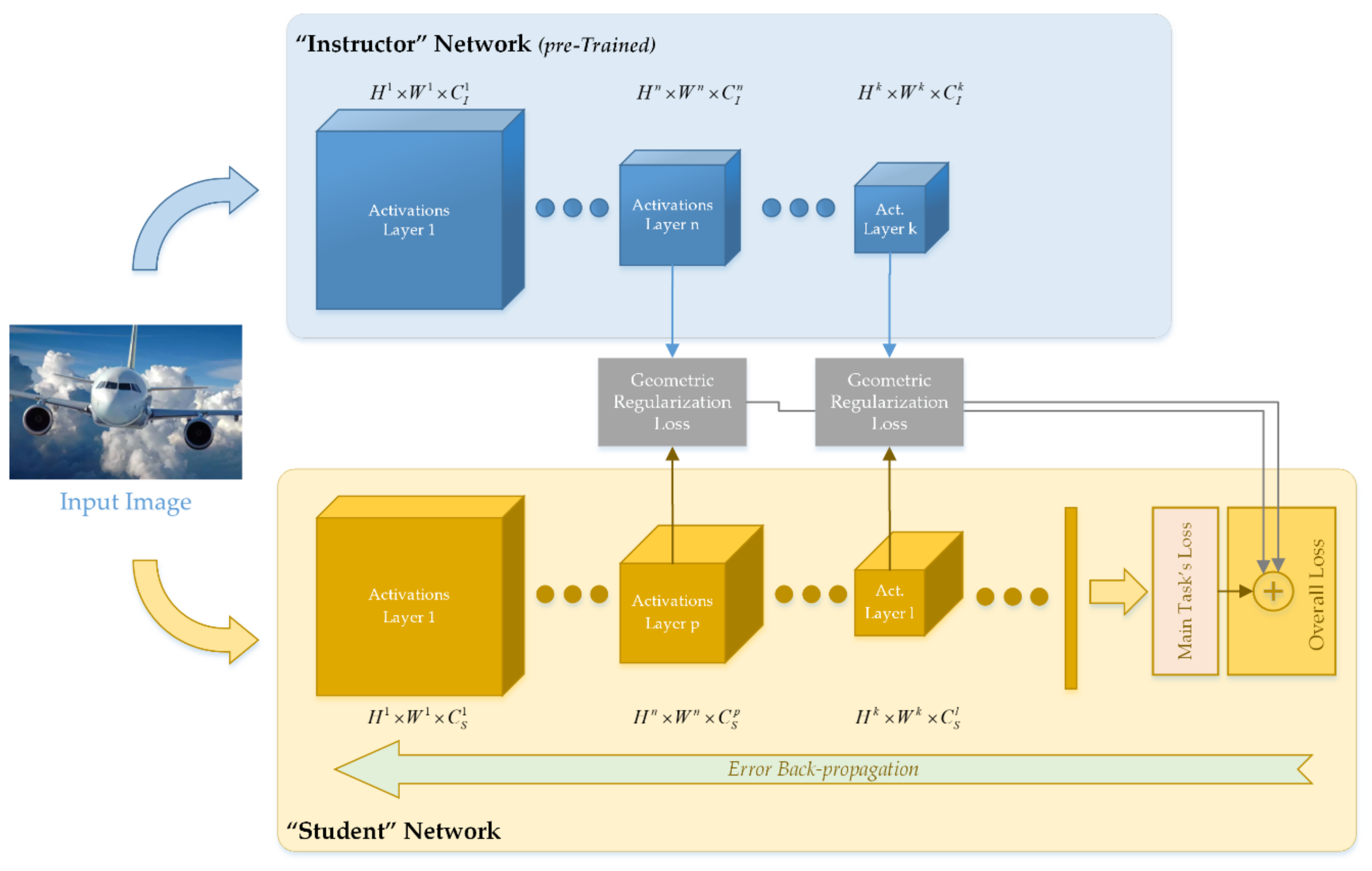
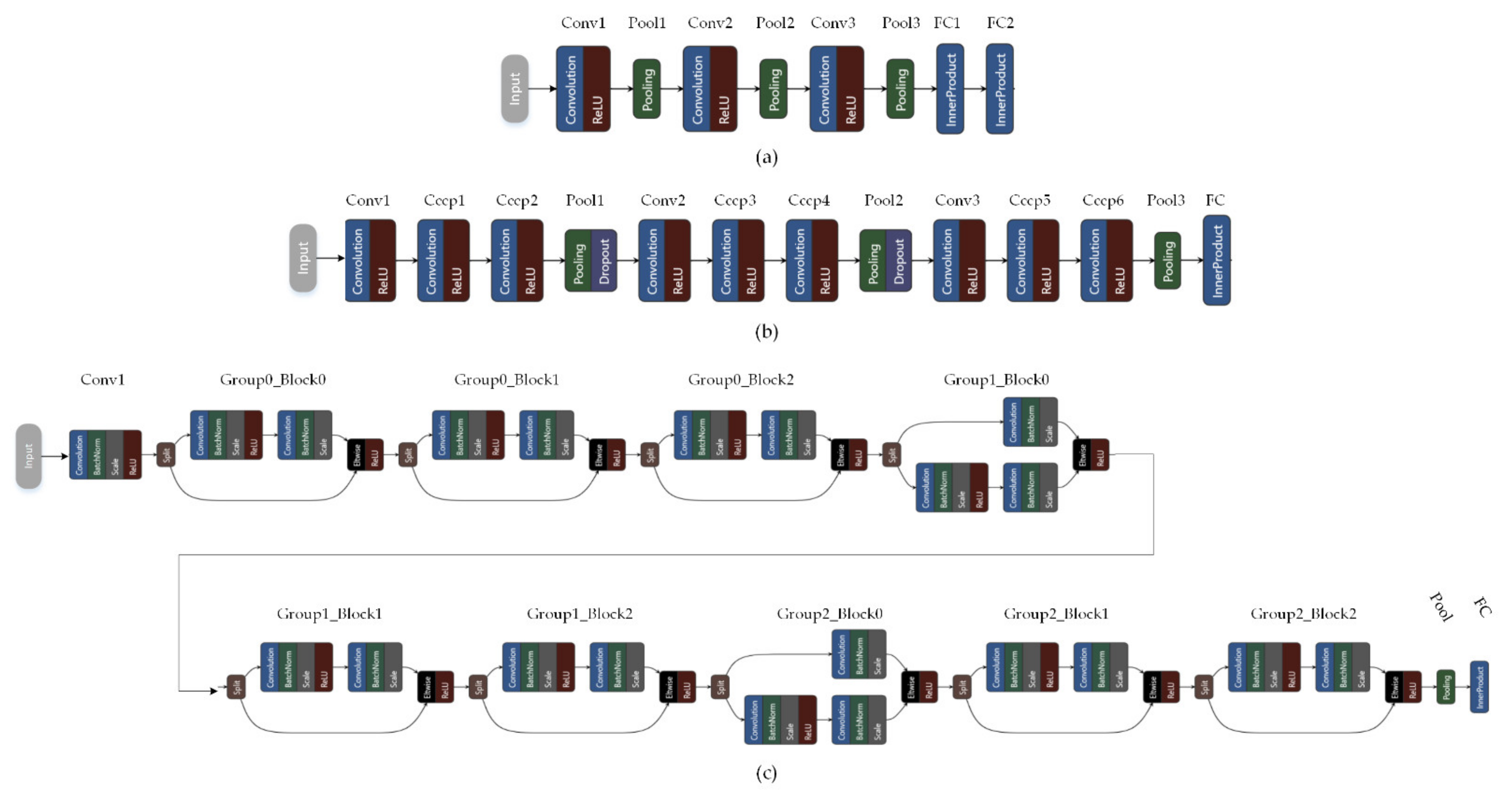
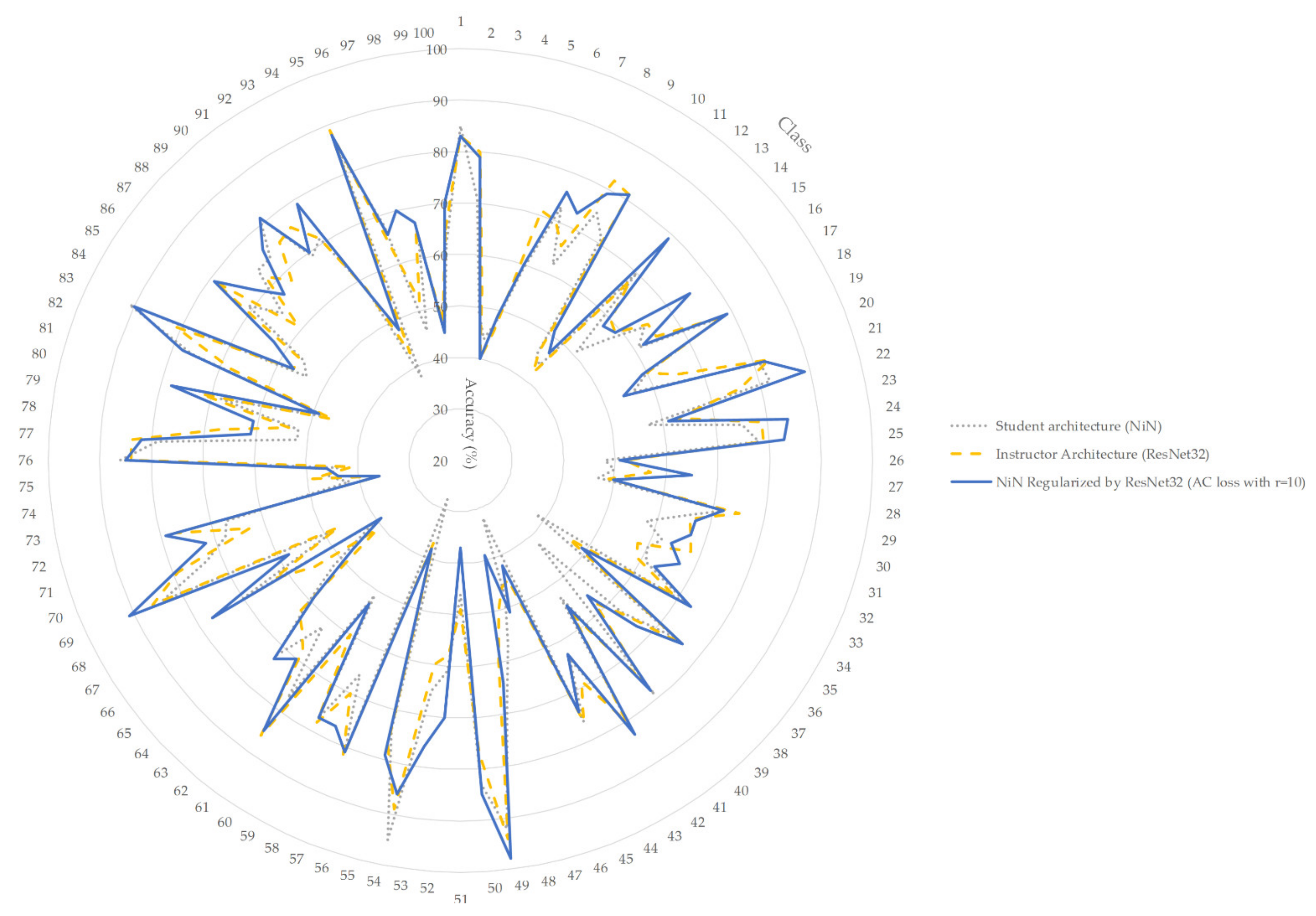
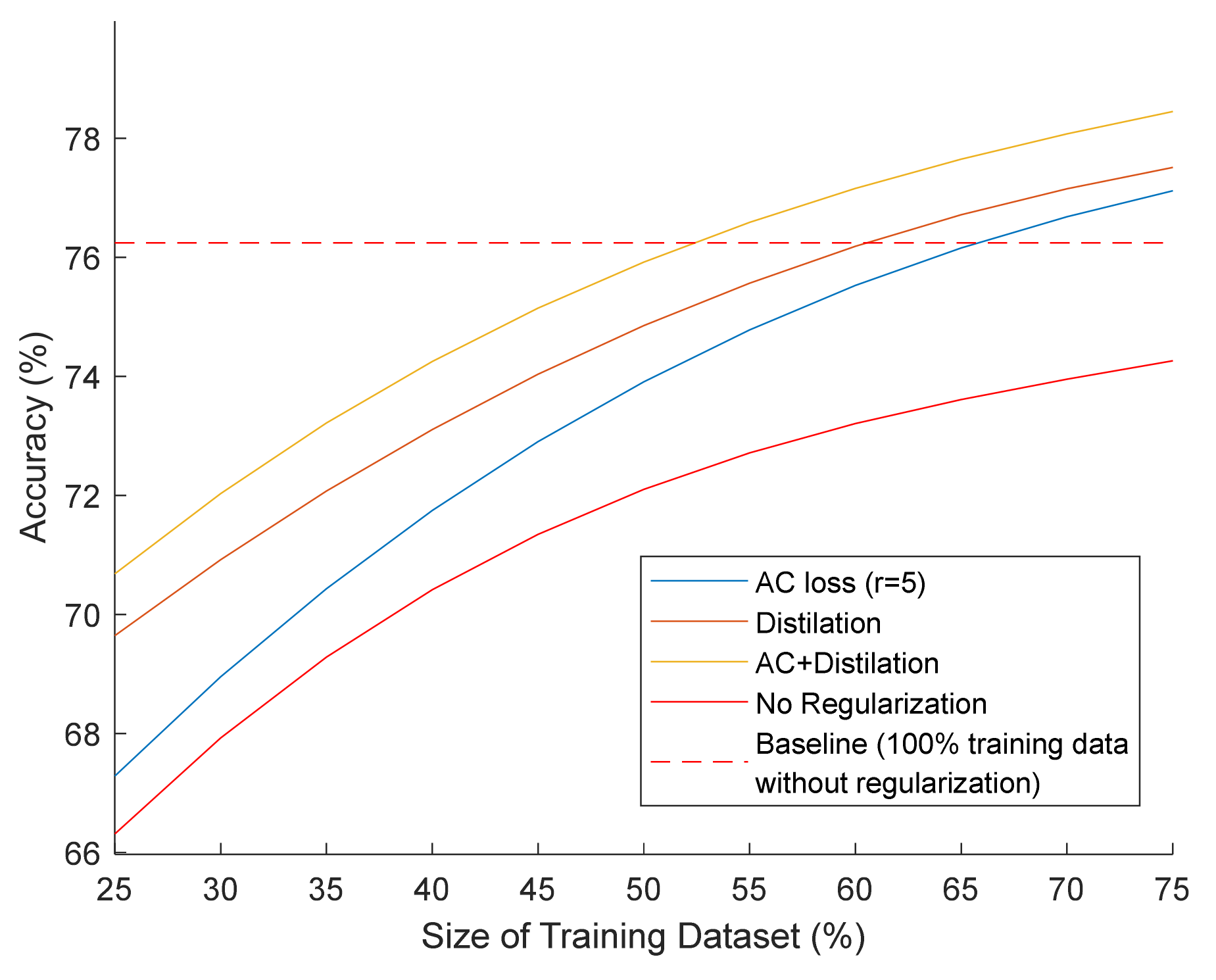
Table 1.
Size of activations at the output of every layer or block for all utilized CNN architectures for 32 × 32 px input dimensions.
Table 1.
Size of activations at the output of every layer or block for all utilized CNN architectures for 32 × 32 px input dimensions.
| Simple CNN | NiN | ResNet-20 | ResNet-32 | ||||
|---|---|---|---|---|---|---|---|
| Layer Name | Activation Size | Layer Name | Activation Size | Layer/Block Name | Activation Size | Layer/Block Name | Activation Size |
| Input | 32 × 32 × 3 | Input | 32 × 32 × 3 | Input | 32 × 32 × 3 | Input | 32 × 32 × 3 |
| Conv1 | 32 × 32 × 32 | Conv1 | 32 × 32 × 192 | Conv1 | 32 × 32 × 16 | Conv1 | 32 × 32 × 16 |
| pool1 | 16 × 16 × 32 | Cccp1 | 32 × 32 × 160 | Group0_block0 | 32 × 32 × 16 | Group0_block0 | 32 × 32 × 16 |
| Conv2 | 16 × 16 × 32 | Cccp2 | 32 × 32 × 96 | Group0_block1 | 32 × 32 × 16 | Group0_block1 | 32 × 32 × 16 |
| pool2 | 8 × 8 × 32 | Pool1 | 16 × 16 × 96 | Group0_block2 | 32 × 32 × 16 | Group0_block2 | 32 × 32 × 16 |
| Conv3 | 8 × 8 × 64 | Conv2 | 16 × 16 × 192 | Group1_block0 | 16 × 16 × 32 | Group0_block3 | 32 × 32 × 16 |
| pool3 | 4 × 4 × 64 | Cccp3 | 16 × 16 × 192 | Group1_block1 | 16 × 16 × 32 | Group0_block4 | 32 × 32 × 16 |
| FC1 | 64 | Cccp4 | 16 × 16 × 192 | Group1_block2 | 16 × 16 × 32 | Group1_block0 | 16 × 16 × 32 |
| FC2 | c | Pool2 | 8 × 8 × 192 | Group2_block0 | 8 × 8 × 64 | Group1_block1 | 16 × 16 × 32 |
| Conv3 | 8 × 8 × 192 | Group2_block1 | 8 × 8 × 64 | Group1_block2 | 16 × 16 × 32 | ||
| Cccp5 | 8 × 8 × 192 | Group2_block2 | 8 × 8 × 64 | Group1_block3 | 16 × 16 × 32 | ||
| Cccp6 | 8 × 8 × 100 | Pool | 64 | Group1_block4 | 16 × 16 × 32 | ||
| Pool | 100 | FC | c | Group2_block0 | 8 × 8 × 64 | ||
| FC | c | Group2_block1 | 8 × 8 × 64 | ||||
| Group2_block2 | 8 × 8 × 64 | ||||||
| Group2_block3 | 8 × 8 × 64 | ||||||
| Group2_block4 | 8 × 8 × 64 | ||||||
| Pool | 64 | ||||||
| FC | c | ||||||
Table 2.
Classification accuracy of the student model (Simple CNN) with regular training versus geometric regularization with AC and NP functions for knowledge transfer from a NiN instructor model. Neighborhoods are defined for radius r on the instructor’s MST. The best obtained accuracy for each dataset is indicated in bold.
| Class. Accuracy (%) | Regular Training | Regularization Function | Neighborhood Radius | |||
|---|---|---|---|---|---|---|
| Dataset/Task | r = 2 | r = 5 | r = 10 | r = ∞ | ||
| CIFAR10 | 76.24 | AC | 77.30 | 77.98 | 78.34 | - |
| NP | 77.03 | 77.21 | 78.00 | 76.14 | ||
| CIFAR100 | 44.49 | AC | 45.14 | 46.71 | 46.1 | - |
| NP | 44.90 | 45.42 | 46.03 | 45.74 | ||
| SVHN | 92.76 | AC | 92.8 | 92.84 | 92.9 | - |
| NP | 92.79 | 92.8 | 92.82 | 92.8 | ||
Table 3.
Number of neighbors for various neighborhood radii using the MST criterion on the NiN instructor models.
Table 3.
Number of neighbors for various neighborhood radii using the MST criterion on the NiN instructor models.
| Activation Layer | Number of Neighbors | |||||
|---|---|---|---|---|---|---|
| r = 2 | r = 5 | r = 10 | ||||
| Mean | Median | Mean | Median | Mean | Median | |
| Conv2 | 5.4 | 5.3 | 36.8 | 22 | 148 | 161 |
| Conv3 | 4.5 | 4.5 | 17.3 | 15 | 45 | 48 |
Table 4.
Comparison of geometric regularization (G. Reg.) of local activations to Knowledge Distillation (Distil.) and their combination.
Table 4.
Comparison of geometric regularization (G. Reg.) of local activations to Knowledge Distillation (Distil.) and their combination.
| Class. Accuracy (%) | Regular Training | G. Reg. AC Loss (Best) | G. Reg. NP Loss (Best) | Knowledge Distillation [4] | AC (r = 5) +Distil. | NP (r = 10) +Distil. |
|---|---|---|---|---|---|---|
| CIFAR10 | 76.24 | 78.34 | 78.00 | 78.25 | 80.03 | 78.61 |
| CIFAR100 | 44.49 | 46.71 | 46.03 | 44.71 | 46.10 | 46.22 |
| SVHN | 92.76 | 92.9 | 92.82 | 92.98 | 93.05 | 92.91 |
Table 5.
Comparison between different neighborhood criteria for geometric regularization with AC loss using the NiN instructor model.
Table 5.
Comparison between different neighborhood criteria for geometric regularization with AC loss using the NiN instructor model.
| Accuracy (%) | MST-Based Neighborhood | k-NN Neighborhood | ||||
|---|---|---|---|---|---|---|
| Dataset | r = 2 | r = 5 | r = 10 | Equiv. to r = 2 | Equiv. to r = 5 | Equiv. to r = 10 |
| CIFAR10 | 77.30 | 77.98 | 78.34 | 76.92 | 77.07 | 78.23 |
| CIFAR100 | 45.14 | 46.71 | 46.1 | 43.87 | 44.87 | 45.05 |
Table 6.
Knowledge transfer via AC loss to student models with NiN architecture, and instructors with ResNet architecture.
Table 6.
Knowledge transfer via AC loss to student models with NiN architecture, and instructors with ResNet architecture.
| Accuracy (%) | Instructor Architecture | Instruct. Accuracy | Regular Training | Regularized w AC Loss | |
|---|---|---|---|---|---|
| r = 5 | r = 10 | ||||
| CIFAR10 | ResNet20 | 91.40 | 86.19 | 88.06 | 88.75 |
| ResNet32 | 92.48 | 88.35 | 88.82 | ||
| CIFAR100 | ResNet32 | 64.95 | 63.24 | 65.80 | 66.40 |
Publisher’s Note: MDPI stays neutral with regard to jurisdictional claims in published maps and institutional affiliations. |
© 2021 by the authors. Licensee MDPI, Basel, Switzerland. This article is an open access article distributed under the terms and conditions of the Creative Commons Attribution (CC BY) license (https://creativecommons.org/licenses/by/4.0/).
Share and Cite
MDPI and ACS Style
Theodorakopoulos, I.; Fotopoulou, F.; Economou, G. Geometric Regularization of Local Activations for Knowledge Transfer in Convolutional Neural Networks. Information 2021, 12, 333. https://0-doi-org.brum.beds.ac.uk/10.3390/info12080333
AMA Style
Theodorakopoulos I, Fotopoulou F, Economou G. Geometric Regularization of Local Activations for Knowledge Transfer in Convolutional Neural Networks. Information. 2021; 12(8):333. https://0-doi-org.brum.beds.ac.uk/10.3390/info12080333
Chicago/Turabian StyleTheodorakopoulos, Ilias, Foteini Fotopoulou, and George Economou. 2021. "Geometric Regularization of Local Activations for Knowledge Transfer in Convolutional Neural Networks" Information 12, no. 8: 333. https://0-doi-org.brum.beds.ac.uk/10.3390/info12080333
Note that from the first issue of 2016, this journal uses article numbers instead of page numbers. See further details here.