
DebtG: A Graph Model for Debt Relationship

College of Computer Science and Engineering, Shandong University of Science and Technology, Qingdao 266590, China
Information 2021, 12(9), 347; https://0-doi-org.brum.beds.ac.uk/10.3390/info12090347
Submission received: 12 August 2021
/
Revised: 23 August 2021
/
Accepted: 25 August 2021
/
Published: 26 August 2021
(This article belongs to the Special Issue Data Modeling and Predictive Analytics)
Abstract
:Debt is common in daily transactions, but it may bring great harm to individuals, enterprises, and society and even lead to a debt crisis. This paper proposes a weighted directed multi-arc graph model DebtG of debts among a large number of entities, including individuals, enterprises, banks, and governments, etc. Both vertices and arcs of DebtG have attributes. In further, it defines three basic debt structures: debt path, debt tree, and debt circuit, and it presents algorithms to detect them and basic methods to solve debt clearing problems using these structures. Because the data collection and computation need a third-party platform, this paper also presents the profit analysis of the platform. It carries out a case analysis using the real-life data of enterprises in Huangdao Zone. Finally, it points out four key problems that should be addressed in the future.
1. Introduction
Currently, debt is flooding people’s lives. Debt is the money borrowed by one entity from another, and it is used by many entities to make large purchases that they could not afford under normal circumstances [1]. In modern society, most of us often buy houses by borrowing from banks or buy some expensive items by installment payment and pay with a credit card. An enterprise often borrows for the needs of production and operation. A country will issue national debt in order to stimulate economic development.
Debt has always been a matter of great concern to governments, but it has been growing recently. Due to the impact of the COVID-19 epidemic in recent two years, the debt scale of countries all over the world has increased rapidly. According to the Institute of International Finance (IIF), the proportion of global government debt in global Gross Domestic Product (GDP) increased from 88% before the epidemic to 105% in 2020, and the total government debt may increase to USD 92 trillion this year. IIF also stated that the global debt increased to USD 281 trillion in 2020, and the ratio of global debt to GDP exceeded 355%, far exceeding the ratio during the international financial crisis in 2008. According to People’s Bank of China (PBC), in 2020, the loan balance of Chinese enterprises reached CNY 110.53 trillion, and the debt ratio exceeded 56%, which is 1.09 times China’s GDP in 2020.
Moderate debt has many advantages. For example, the government debt can make up the fiscal deficit, and the enterprise can use debt to increases access to new opportunities for expansion. However, debt increases the risk of insolvency, and debt forms a central part of the narrative of financial crises [2]. In further, the number of entities involved in debt is very large, and the relationship is very complex, so it is necessary to model the debt relationship.
It relies on a third-party platform to collect and process a large amount of debt information. As debt is one of the business secrets of enterprises, this platform must be highly credible and recognized by all entities. Meanwhile, the platform should be able to make profits when settling debts to maintain its operation. This platform may be the Ministry of Finance [3] or the subsidy center [4].
This paper constructs a graph model DebtG of a large number of debt relationships and points out the potential applications and key techniques of DebtG. The main contributions of the paper are as follows:
- It presents a graph model of debt relationship between entities including individuals, enterprises, governments, etc.;
- It defines three basic debt structures, namely debt path, debt tree, and debt circuit;
- It proposes two algorithms to detect the three debt structures and possible methods to solve the debt clearing problem based on these structures;
- It carries out a profit analysis of the third-party platform and presents a case analysis using real-life debt data.
The organizations of the rest of the paper are as follows. Section 2 introduces related works. Section 3 presents the DebtG model and its application, including the definitions of three debt structures and methods to detect and resolve them. Section 4 provides the profit analysis and case analysis. Section 5 concludes the paper and points out future works.
2. Related Works
Much of the literature focused on debt. L. Wang et al. [5] examined the relation between three dimensions of national culture and debt risk using a sample of 65 “Belt and Road” countries during the period from 2008 to 2017. Q. Ye et al. [6] analyzed the causes of local government debt in China by combing the development process of debt and relevant debt management policy measures, and then they put forward some suggestions on improving local government debt risk management mechanisms. C. Wang et al. [7] took five countries as examples to examine the relation between a firm’s short-term debt and its default probability.
Different from the above literature, this paper focuses on the model of debt relationship and explores the potential applications in the debt clearing problem. The model is based on a graph. As an important model to represent the complex relationships among entities, graphs are widely applied in many fields [8]. In economic and financial fields, the financial system can be modeled as a weighted directed graph to simulate and analyze the impact of financial regulations on systemic risk [9]. Q. Zhan et al. [10] combined knowledge graphs and machine learning to detect consumer finance fraud. A. Gogoglou et al. [11] formulated the credit card transactions as a bipartite graph between account holders and the merchants they shop at. Y. Ren et al. [12] utilized a bipartite graph to model the relationship between users and merchants and proposed an ensemble-based fraud detection method. S. Yang et al. [13] applied a temporal graph to model financial relationships between enterprises to analyze financial risk.
A graph is also used for modeling and theoretical research of debt clearing problems. V. Gazda [3] modeled the creditor–debtor relations as a weighted directed graph in order to deal with the firms’ financial insolvency as a result of their mutual debts. V. Gazda et al. [4] further demonstrated that the debt compensation is related to the optimization problem maximizing the circulation of the consecutive compensation in the digraph of debts. They formulated this optimization problem by linear programming methods and applied Klein’s cycle-canceling algorithm to solve it. C. Patcas et al. [14] also applied a weighted directed graph to model the debt relationship, but they described an evolutionary algorithm to solve the debt clearing problem based on the graph. L. Liang et al. [15] transferred all debts to the forward debt chain and backward debt chain and proposed an algorithm to simplify both debt chains.
The graph models used in the above references are all simple graphs; that is, there is at most one arc between two vertices, and they often aim to find or construct a cycle to solve the problem of mutual debt compensation or debt clearing. There are still some gaps between these ideal models and the actual situation:
- The entities involved in debt relationships have many attributes that affect debt clearing. For example, the due date of debt is more important than the amount of debt in determining the order of debt settlement. However, the current models only focus on the debt amount in order to clear the largest amount of debt;
- There is often more than one debt between a pair of entities, and these debts also have different attributes. An entity may prefer to settle earlier debts with higher discounts or vice versa. However, the current models only contain at most one debt between a pair of entities;
- It may be impossible to solve the debt clearing problem by constructing cycles with the help of the Ministry of Finance (see [3]) or subsidy center (see [4]). When the series of entities formed a debt path (see Section 3), refs. [3,4] added a third-party platform to the path to construct a cycle, and the platform paid the first debtor to clear the debts. However, the last creditor had no obligation to pay the platform because it did not owe the platform.
3. DebtG Model and Its Application
This section presents the formal definition of DebtG and its potential applications to deal with the debt problem.
3.1. Formal Definitions
In DebtG, the entities involved in debts are represented by vertices, and their debt relationships are represented by directed arcs. If entity A owes entity B, there is an arc from the corresponding vertex of A to that of B. Both vertices and arcs have attributes. The formal definition of DebtG is as follows.
Definition 1.
(DebtG) A DebtG is a weighted directed multi-arc graph , where:
- is the set of vertices, and each vertex represents an entity (for example, enterprise, government, individual, bank, etc.). Each vertex has a unique ID;
- is the set of directed arcs, and each arc represents the corresponding entities have debt relationship. Specifically, denotes that the corresponding entity of owes that of . There may exist more than one arc between a pair of entities;
- is the attribute sets of vertices, and is the attribute set of . The attribute sets of vertices contain the name, address, assets, and other information of corresponding entities;
- is the attribute sets of arcs, and is the attribute set of . The attribute sets of arcs should contain the amount of debt, and it may also contain the debt arising/due date, priority, and other information of debt.
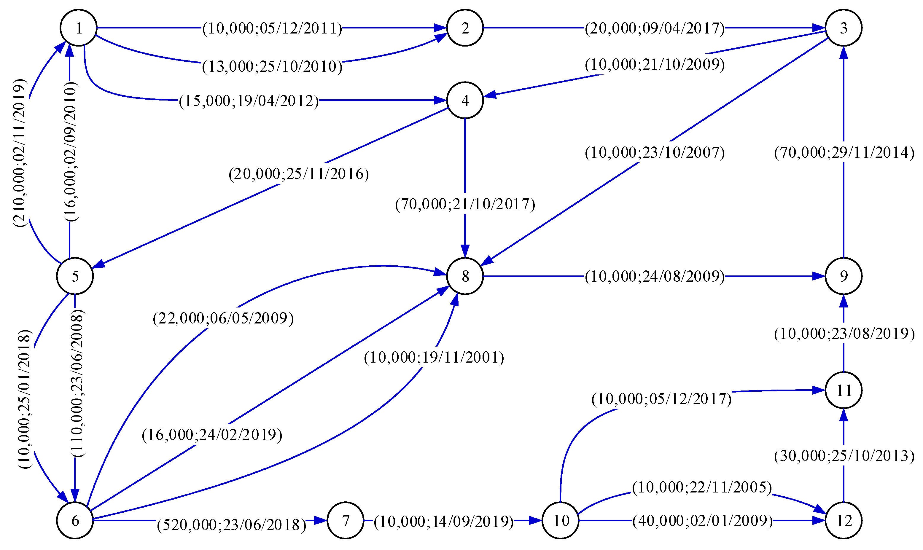
Figure 1 is a simple example of DebtG, which only exhibits a part of attributes of vertices and arcs due to the limited space of the figure. It has 12 vertices and 24 arcs. The arcs contain two attributes , where is the amount of debt and is the debt arising/due date.
Definition 2.
(Degree) Given DebtG , the degree of vertex is:
- Out-degree denotes is the debtor of entities;
- In-degree denotes is the creditor of entities.
3.2. Debt Structures of DebtG
The main application of DebtG is to mine the relationship among a large number of entities to find the possible method to solve debt clearing problems. This paper mainly focuses on the following three debt structures.
Definition 3.
(debt path) A sequence of vertices is a debt path if it satisfies for , and for , . The first vertex is called the path head, and the last vertex is called the path end.
Definition 4.
(debt circuit) A debt path is a debt circuit if . Given a debt circuit, the minimal amount of debt of all arcs is called the settle amount.
Definition 5.
(debt tree) A debt tree is composed of multiple debt paths with a common path head, and any sequence of vertices does not form a debt circuit. The common path head is called tree root.
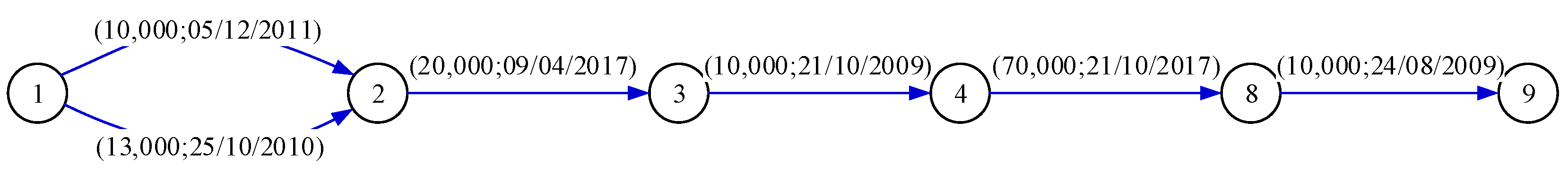
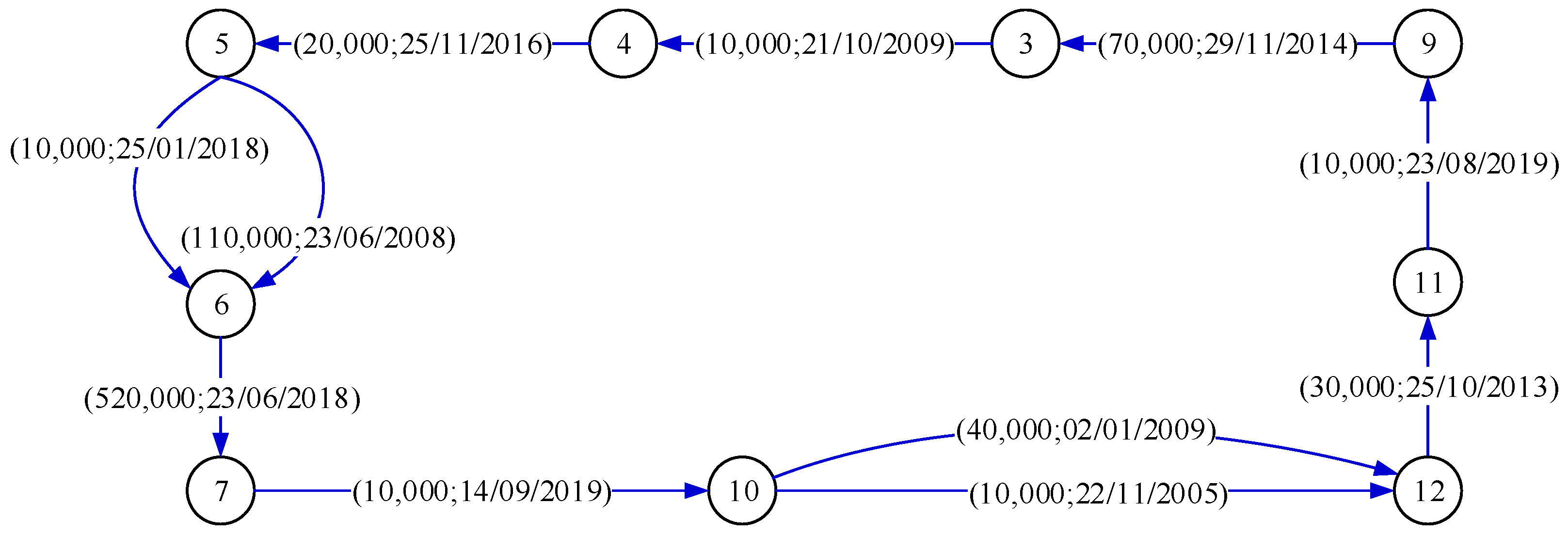
Figure 2, Figure 3 and Figure 4 present examples of a debt path, debt circuit, and debt tree, respectively. Note that the debt path and debt circuit are, respectively, the extensions of path and cycle in graph theory, where the “extension” means all arcs between two neighboring vertices should be included in the debt path and debt circuit. The debt tree is different from the directed tree in graph theory. In graph theory, a directed tree is a directed graph that would be connected and acyclic if the directions on the arcs were ignored. In DebtG, the debt tree is connected but cyclic if the directions on the arcs were ignored. For example, the debt tree in Figure 4 has a cycle {1,2,3,4}, so it is not a directed tree in graph theory.
3.3. Detection and Elimination of Debt Circuit
Debt circuit was studied in [3,4] as the problem of mutual debt compensation, but these references did not present the method of debt circuit detection. Additionally, refs. [3,4] tried to detect all debt circuits, which is very difficult for large-scale DebtG. According to experiments in Section 4.2, some debt circuits share at least one common arc. If this common arc is broken when the corresponding debt is cleared, these debt circuits are all broken. Moreover, the detection of all debt circuits is too expensive computationally, even for a small-scale graph [4]. Therefore, it is not necessary to detect all debt circuits, and a debt circuit should be eliminated immediately after it is detected.
Based on the above idea, Algorithm 1 presents the procedure to detect and eliminate debt circuits.
| Algorithm 1 Detect and Eliminate Debt Circuits | |
| Required: A DebtG | |
| Ensure: A set of debt circuits | |
| 1. | for each do |
| 2. | |
| 3. | |
| 4. | end for |
| 5. | |
| 6. | for each do |
| 7. | if then |
| 8. | |
| 9. | else if then |
| 10. | |
| 11. | end if |
| 12. | if or then |
| 13. | |
| 14. | end if |
| 15. | delete and its associate arcs from |
| 16. | |
| 17. | end for |
| 18. | while do |
| 19. | Sort according to a certain criterion |
| 20. | the first vertex in |
| 21. | detect a debt circuit starting with |
| 22. | if exists then |
| 23. | |
| 24. | subtract from all attributes of all arcs of |
| 25. | else |
| 26. | |
| 27. | end if |
| 28. | end while |
| 29. | return all debt circuits |
Algorithm 1 calculates the degrees of vertices in first (lines 1–4). Lines 5–17 iteratively remove the vertices whose out- or in-degree is 0 because these vertices will not form a debt circuit.
Line 19 sorts the vertices according to a certain criterion. The criterion may be the amount of debt, enterprise scale, debt arising/due date, or composition. This criterion is very important because it decides the order of eliminating debt circuits.
Line 20 fetches a vertex as the starting one to detect the debt circuit. Line 21 detects the debt circuit. Because a debt circuit is a cycle of a graph, and the cycle detection algorithms can be found in many places, such as [16], so the specific details are not given. Lines 22–25 eliminate the debt circuit whose idea is the same as [4]. Line 23 calculates the settle amount of this circuit, and line 24 eliminates the detected debt circuit. If it cannot detect debt circuits from vertex , line 26 deletes .
Taking Figure 3 as an example, its settle amount is 10,000. Therefore, the platform transfers 10,000 to vertex 5, and then vertex 5 pays 10,000 to vertex 6, and so on. Finally, vertex 4 pays 10,000 to vertex 5, and vertex 5 returns 10,000 to the platform. The above method clears the debt of 10,000 between two neighboring vertices, and the debts , and are completely cleared. The debt circuit is broken.
The differences between Algorithm 1 and traditional cycle detection algorithms include: (1) Algorithm 1 removes the vertices whose out- or in-degree is 0 in first while existing algorithms do not; (2) Algorithm 1 clears a debt circuit once it is detected, while existing algorithms try to detect all cycles and choose the best one to clear.
3.4. Detection and Clearing of Debt Tree and Debt Path
Debt path can be regarded as a special case of debt tree, so debt trees and debt paths can be detected and cleared simultaneously. Because debt circuits were eliminated from DebtG, Algorithm 2 presents the procedure of detecting and clearing debt trees and debt paths for an acyclic graph. The basic idea is to start from one vertex and detect all the reachable vertices from . We say that a vertex is reachable from a vertex if there exists a directed path from to .
| Algorithm 2 Detect and Clear Debt Trees and Debt Paths | |
| Required: An acyclic DebtG | |
| Ensure: A set of debt trees and debt paths | |
| 1. | Sort according to a certain criterion |
| 2. | candidate tree roots and path heads |
| 3. | for each do |
| 4. | is a queue |
| 5. | is the list of vertices of a debt tree or debt path |
| 6. | while is not empty do |
| 7. | |
| 8. | for each and do |
| 9. | |
| 10. | |
| 11. | end for |
| 12. | end while |
| 13. | for each do |
| 14. | |
| 15. | end for |
| 16. | |
| 17. | |
| 18. | while is not empty do |
| 19. | |
| 20. | for each or do |
| 21. | if then |
| 22. | |
| 23. | end if |
| 24. | end while |
| 25. | resolve the debt tree or debt path according to values of all vertices |
| 26. | end for |
In Algorithm 2, line 1 sorts the vertices according to a certain criterion, where the sorting criterion may be the same as that of line 19 of Algorithm 1. Line 2 decides candidate tree roots and path heads. The entities who are willing and able to repay all or part of their debts are candidates, and the money they pay clear more debts by flowing through the debt tree or debt path. Lines 3–26 detect and clear the debt trees and debt paths from each candidate tree root and path head.
In this algorithm, is a queue, , and are two basic operations of the queue. fetches and removes the first element from , and adds to . records the list of vertices of a debt tree or debt path.
Lines 4–5 initialize and . Lines 6–12 compute the debt tree ( is the tree root) or debt path ( is the path head). When is not empty, line 7 fetches a vertex from , and lines 8–11 append the neighboring vertices of to and .
For each vertex , is its topological sort order. Lines 13–15 initialize to 0 for each . Line 16 sets ( is the debt tree root or debt path head) to 1, and line 17 enqueues to . Lines 18–24 calculate the topological orders of all vertices of . Line 25 clears the debt tree or debt path according to the topological orders. There are two ways to clear debt trees and debt paths:
- If the tree root or path head pays enough money, this money can flow along the debt tree or debt path according to the topological orders of vertices. Taking Figure 4 as an example, suppose vertex 1, respectively, pays 15,000 to its creditors, vertices 2 and 4. Next, vertex 2 pays 15,000 to vertex 3, and vertex 3 pays 10,000 to vertex 4, so vertex 4 has 25,000. Vertex 4 pays 20,000 to vertex 6 through vertex 5, and vertex 6, respectively, pays 10,000 to vertex 8 and vertex 10 (through vertex 7) finally. During the above procedure, if a vertex in the debt tree can afford additional money, the successive users can receive more money. Because the topological order of vertex 4 is larger than that of vertex 3, vertex 4 should pay vertex 5 after it receives from vertex 3;
- Each vertex of the debt tree or debt path contributes some money to the third-party platform to aggregate enough money, and the platform pays it to the tree root or path head. The subsequent solution is the same as the above procedure. Taking Figure 2 as an example, vertices 1, 2, 3, and 9, respectively, contribute 2000, vertices 4 and 8, respectively, contribute 1000. Finally, these vertices gather 10,000 and pay to the platform, and then the platform pays 10,000 to vertex 1. This method is similar to crowdfunding.
4. Profit and Case Analysis
4.1. Profit Analysis
As mentioned above, the collection and clearing of debts rely on the third-party platform. The platform needs to make some profit to maintain its operation. The profit model of the debt circuit is simple: the platform can charge the entity’s service fee of the debt circuit. Due to Algorithm 1 improving the efficiency of clearing debt circuits, the platform can detect and settle more debt circuits than existing methods.
This paper puts forward the concepts and settling methods of debt tree and debt path for the first time. These two new structures enhance the ability and scope of the platform to settle debt problems so that the platform can benefit from them. For debt tree or debt path, the platform can advance part of the money to tree root or path head to motivate more entities to participate in crowdfunding. Since the debt path is a special case of a debt tree, the profit model of the debt path is analyzed. Let , , and , respectively, be the amount paid by path head, the amount advanced by platform, and the platform’s profit. Let be service fee rate. Therefore, each entity needs to take a part of the receipt as the service fee of the platform according to . Suppose each vertex of a debt path transfers all of what it received. Given a debt path , pays to . Next, pays to platform as the platform’s profit and pays to . Obviously, the amount of user receives from the previous user is
Subsequently, needs to pay
to the platform as the platform’s profit, and needs to pay
to if . Therefore, the profit of the platform is
According to Equation (4), the platform is profitable if and only if . If is known prior, we need estimate . implies
Define function as
We have
so is monotonic increasing on and . Figure 5 presents the figure of when = 100. Using , the upper limit of can be calculated. If satisfies Equation (5) for a given , the platform is profitable.
4.2. Case Analysis
We used the debt data collected in Huangdao Zone, Shandong Province, China, to carry out the case analysis. The data contained 7664 entities and 8704 debts; the total amount of debt is CNY 1.61 billion.
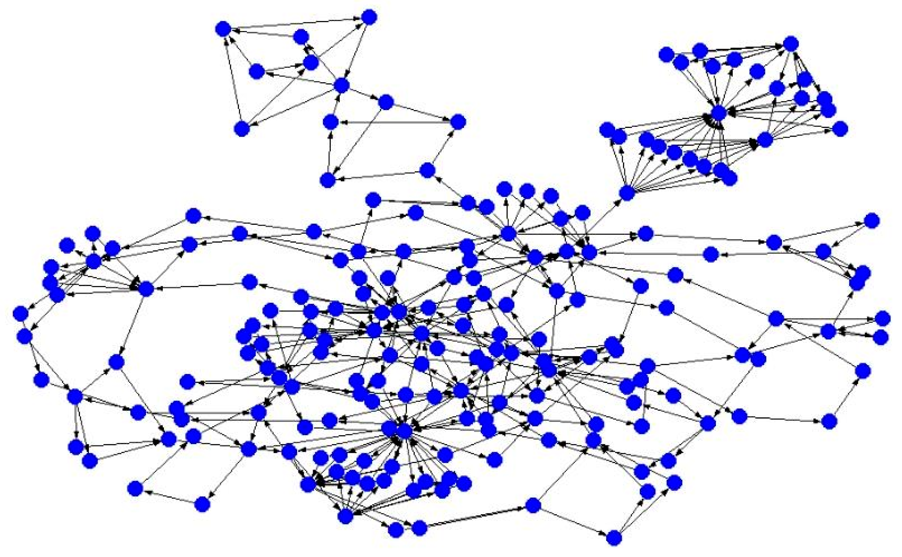
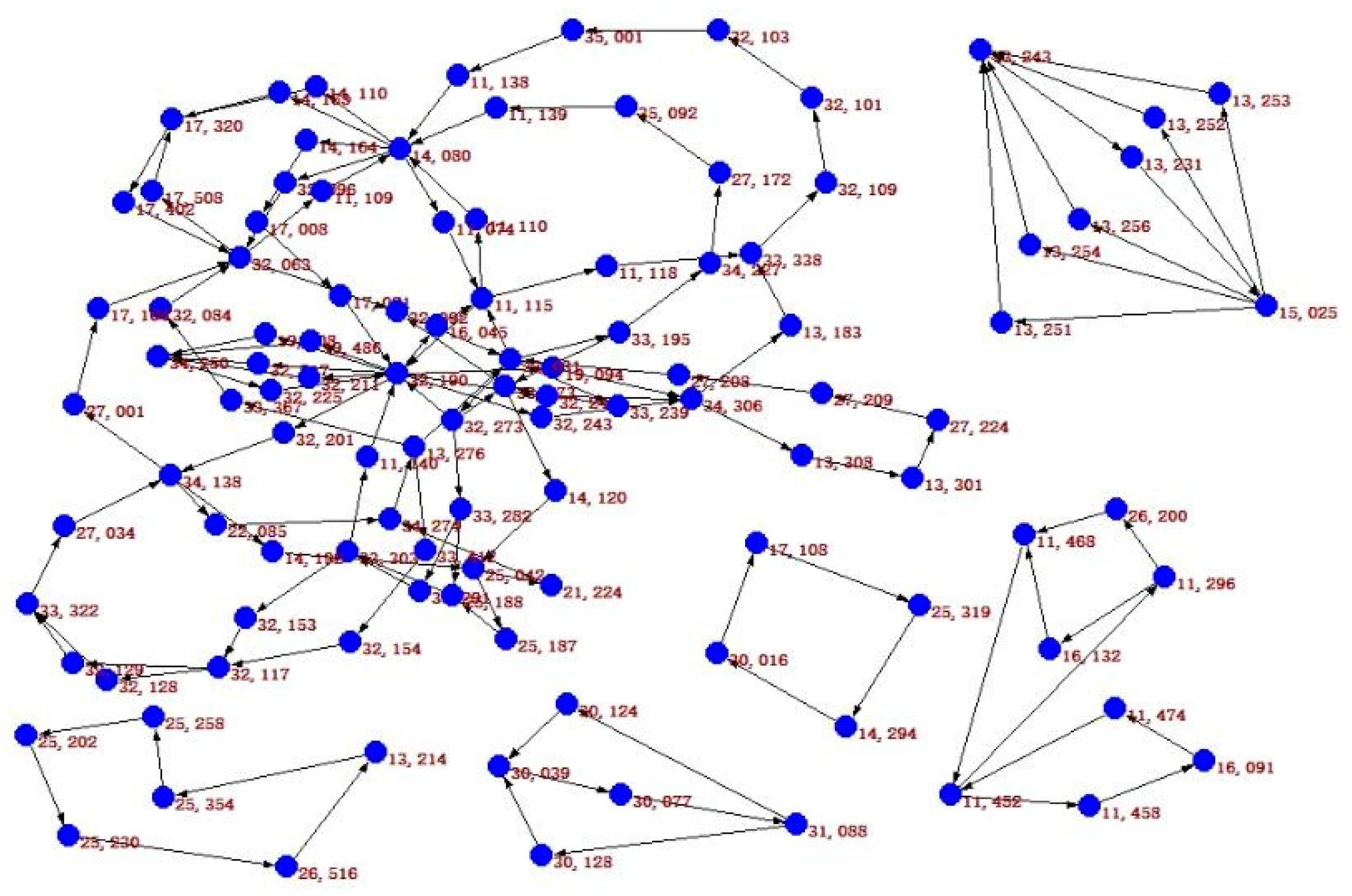
Using Algorithm 1 to detect the debt circuits, DebtG remains 201 vertices and 372 arcs after removing the vertices whose in- or out-degree is 0 iteratively (lines 5–17), as shown in Figure 6. Figure 7 shows the debt circuits detected by Algorithm 1. These debt circuits can clear CNY 13.35 million debts.
Table 1 presents the details of these 40 debt circuits. In Table 1, the “sequence of vertices” is the IDs of entities involved in a debt circuit, and the “settle amount” is the settle amount of the corresponding debt circuit. For example, the second row means (15,025–13,256–13,243–13,231–15,025) is a debt circuit, and its settle amount is CNY 33,000. We can see that some debt circuits share common arcs. For example, the debt circuits of the second to sixth rows share a common arc <13,243;13,231>.
We tried to find all debt circuits in Figure 6 using a computer with Intel Core i5 CPU and 8GB memory, but the program cannot finish in 30 min, and it detects hundreds of debt circuits, many of which share common arcs. Due to the long runtime and many redundant results, Algorithm 1 eliminates a debt circuit immediately after it is detected.
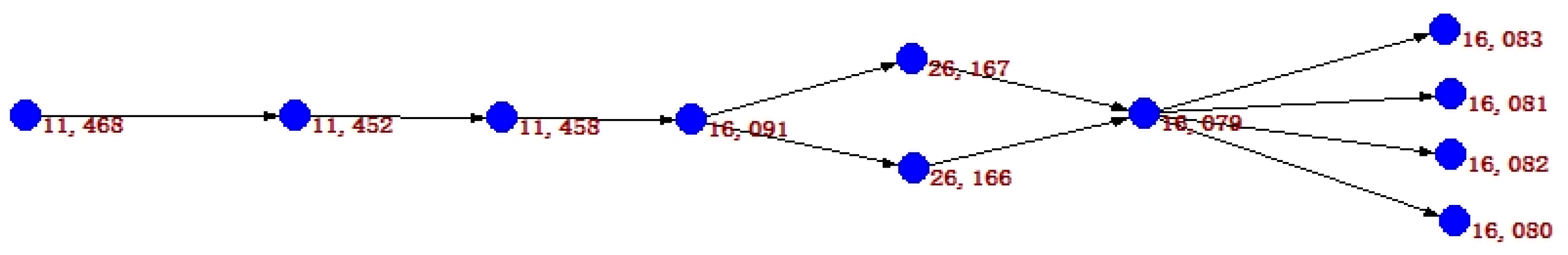
After eliminating debt circuits from DebtG, it becomes acyclic. Given a vertex or a list of vertices as tree root or path head, Algorithm 2 detects the debt trees and debt paths. Starting from user 11,468, a debt tree shown in Figure 8 is detected.
5. Conclusions and Discussions
Many enterprises and countries are concerned about rapid and accurate debt clearing. However, each debtor is unable to understand the overall picture in the absence of comprehensive and accurate debt data.
This paper constructs a graph model DebtG of debt relationship between massive entities (individuals, enterprises, governments, etc.). Furthermore, it defines three possible debt structures: debt path, debt circuit, and debt tree, and it proposes algorithms and basic methods to detect and clear these debt structures.
Based on DebtG, the government can establish a department as the third-party platform mentioned in this paper, and then the platform can solve the debt clearing problem as much as possible using the algorithms proposed in this paper. On the one hand, the profit analysis proves that this platform can be profitable, which will be a potential emerging industry. On the other hand, the settlement of a large number of debts is conducive to the healthy, rapid, and sustainable development of the economy.
The proposed algorithms were applied by YouRong Information Technology Co., Ltd., located in Qingdao, China. Based on tens of thousands of debt information collected from more than 1000 enterprises, YouRong solved more than 2000 debts of them, with a total amount of debt of more than CNY 100 million and a profit of more than CNY 1 million.
However, there are still many problems that need to be addressed in the future:
- The sorting criterion of entities (also the vertices of DebtG). Each entity wants to clear its debts first, but the debt structures are conflicting, as shown in the case analysis, so priority should be decided to guide the detection of debt structures;
- Privacy-preserving strategies during debt data collection. Debt is entities’ privacy, so it is very important to provide extremely privacy-preserving strategies;
- Methods to ensure that money flow only in the debt structure. The money provided by the third-party platform and/or tree root or path head aims to clear a series of debts of a debt structure, so it is very important to ensure that this money only flows between neighboring entities (also the vertices of DebtG) in a given debt structure;
- Algorithms to deal with large-scale graphs. Obviously, the more debt information is collected, the larger the DebtG is constructed, and the more debt are cleared. The large-scale graph needs effective distributed algorithms running on distributed systems.
Funding
This research was funded by Qingdao Social Science Planning Research Project, grant number QDSKL1901122, and Science and Technology Support Plan of Youth Innovation Team of Shandong Higher School, grant number 2019KJN024.
Data Availability Statement
The debt data used in this paper are available at https://figshare.com/articles/dataset/data_txt/14547432/1 (doi:10.6084/m9.figshare.14547432.v1, accessed on 6 May 2021).
Conflicts of Interest
The authors declare no conflict of interest.
References
- Almenberg, J.; Lusardi, A.; Säve-Söderbergh, J.; Vestman, R. Attitudes towards Debt and Debt Behavior. Scand. J. Econ. 2020, 123, 780–809. [Google Scholar] [CrossRef]
- Drehmann, M.; Illes, A.; Juselius, M.; Santos, M. How much income is used for debt payments? A new database for debt ser-vice ratios. BIS Q. Rev. 2015. Available online: https://ssrn.com/abstract=2661611 (accessed on 6 May 2021).
- Gazda, V. Mutual Debts Compensation as Graph Theory Problem. In Topics in Numerical Partial Differential Equations and Scientific Computing; Springer: Berlin, Germany, 2001; pp. 162–167. [Google Scholar]
- Gazda, V.; Horváth, D.; Rešovský, M. An application of graph theory in the process of mutual debt compensation. Acta Poly-Tech. Hung. 2015, 12, 7–24. [Google Scholar]
- The Effect of National Culture on Debt Risk: An Empirical Analysis of “Belt and Road” Countries. In Proceedings of the 2020 International Conference on Big Data Application & Economic Management (ICBDEM 2020), Guiyang, China, 18 September 2020; Francis Academic Press: London, UK, 2020; pp. 470–481.
- Ye, Q.; Chen, M. Research on the Risk of Local Government Debt in China in the New Era. In Proceedings of the 2nd International Conference on Economy, Management and Entrepreneurship (ICOEME 2019), Voronezh, Russia, 14–15 May 2019; Atlantis Press: Dordrecht, The Netherlands, 2019; pp. 197–202. [Google Scholar]
- Wang, C.-W.; Chiu, W.-C. Effect of short-term debt on default risk: Evidence from Pacific Basin countries. Pac.-Basin Financ. J. 2019, 57, 101026. [Google Scholar] [CrossRef]
- Majeed, A.; Rauf, I. Graph Theory: A Comprehensive Survey about Graph Theory Applications in Computer Science and Social Networks. Inventions 2020, 5, 10. [Google Scholar] [CrossRef] [Green Version]
- O’Halloran, S.; Nowaczyk, N.; Gallagher, D. Big Data and Graph Theoretic Models. In Proceedings of the 2017 IEEE/ACM International Conference on Advances in Social Networks Analysis and Mining 2017, Sydney, Australia, 31 July–3 August 2017; Association for Computing Machinery (ACM): New York, NY, USA, 2017; pp. 1056–1064. [Google Scholar]
- Zhan, Q.; Yin, H. A loan application fraud detection method based on knowledge graph and neural network. In Proceedings of the 2nd International Conference on Cryptography, Security and Privacy, Guiyang, China, 16–19 March 2018; Association for Computing Machinery (ACM): New York, NY, USA, 2018; pp. 111–115. [Google Scholar]
- Gogoglou, A.; Nguyen, B.; Salimov, A.; Rider, J.; Bayan Bruss, C. Navigating the dynamics of financial embeddings over time. arXiv 2020, arXiv:2007.00591. [Google Scholar]
- Ren, Y.; Zhu, H.; Zhang, J.; Dai, P.; Bo, L. EnsemFDet an Ensemble: Approach to Fraud Detection based on Bipartite Graph. In Proceedings of the 2021 IEEE 37th International Conference on Data Engineering (ICDE) 2021, Chania, Greece, 19–22 April 2021. [Google Scholar]
- Yang, S.; Zhang, Z.; Zhou, J.; Wang, Y.; Sun, W.; Zhong, X.; Fang, Y.; Yu, Q.; Qi, Y. Financial Risk Analysis for SMEs with Graph-based Supply Chain Mining. In Proceedings of the Twenty-Ninth International Joint Conference on Artificial Intelligence, Yokohama, Japan, 11–17 July 2020; pp. 4661–4667. [Google Scholar]
- Păatcaş, C.; Bartha, A. Evolutionary solving of the debts’ clearing problem. Acta Univ. Sapientiae Inform. 2019, 11, 142–158. [Google Scholar] [CrossRef] [Green Version]
- Liang, L.; Chen, S.; Wu, D.D. A Decision Support Approach to Liquidate a Distressed Debt Network. IEEE Trans. Syst. Man Cybern. Syst. 2017, 50, 1242–1251. [Google Scholar] [CrossRef]
- Deo, N. Graph theory with applications to engineering and computer science. Networks 1975, 5, 299–300. [Google Scholar] [CrossRef]
Figure 1.
Example of DebtG.

Figure 2.
Example of debt path.

Figure 3.
Example of debt circuit.

Figure 4.
Example of debt tree.

Figure 5.
Example of with = 100.

Figure 6.
Graph after removing vertices of in-/out-degree 0.

Figure 7.
Debt circuits of Figure 6.
Figure 7.
Debt circuits of Figure 6.

Figure 8.
A debt tree starting from 11,468.


Table 1.
Details of debt circuits in Figure 6.
Table 1.
Details of debt circuits in Figure 6.
| Sequence of Vertices | Settle Amount |
|---|---|
| 33,338–32,109–32,101–32,103–35,001–11,138–14,080–14,164–17,008–17,021–32,190–19,094–34,306–13,183 | 0.9 |
| 15,025–13,256–13,243–13,231 | 33.0 |
| 15,025–13,251–13,243–13,231 | 23.0 |
| 15,025–13,254–13,243–13,231 | 18.0 |
| 15,025–13,253–13,243–13,231 | 11.0 |
| 15,025–13,252–13,243–13,231 | 12.0 |
| 11,452–11,458–16,091–11,474 | 10.0 |
| 11,468–11,452–11,296–26,200 | 5.0 |
| 16,132–11,468–11,452–11,296 | 7.0 |
| 25,230–26,516–13,214–25,354–25,258–25,202 | 10.0 |
| 32,063–17,508–17,320–17,402 | 6.28 |
| 33,031–33,195–33,473–14,120–25,042–21,224–34,274–13,276–33,367–32,084–32,063–32,092 | 8.0 |
| 33,031–33,195–33,473–14,120–25,042–21,224–34,274–13,276 | 12.0 |
| 14,080–14,164–17,008–17,021–32,190–19,094–34,306–13,308–13,301–27,224–27,209–27,208–33,031–33,195–34,227–27,172–35,092–11,139 | 3.0 |
| 32,190–19,094–34,306–13,308–13,301–27,224–27,209–27,208–33,031–32,273 | 5.0 |
| 32,190–19,094–34,306–13,308–13,301–27,224–27,209–27,208–33,031–32,273–33,282–33,291–33,303–11,140 | 0.4 |
| 32,190–19,094–34,306–13,308–13,301–27,224–27,209–27,208–33,031–32,273–33,282–25,188–33,303–11,140 | 1.9 |
| 33,031–32,273–33,473–32,092 | 0.9 |
| 32,190–19,094–34,306–13,308–13,301–27,224–27,209–27,208–33,031–11,115 | 5.3 |
| 32,190–32,217–34,250–32,225 | 9.0 |
| 32,190–32,243–34,306–13,308–13,301–27,224–27,209–27,208–33,031–11,115 | 3.0 |
| 32,190–32,211–34,250–32,225 | 3.0 |
| 32,190–32,201–34,138–27,001–17,104–32,063–32,092–33,031–11,115 | 9.0 |
| 32,190–32,245–34,306–13,308–13,301–27,224–27,209–27,208–33,031–11,115 | 7.0 |
| 32,190–19,508–34,250–32,225 | 9.0 |
| 32,190–19,486–34,250–32,225 | 5.0 |
| 32,190–16,045–11,115 | 1.0 |
| 33,338–32,109–32,101–32,103–35,001–11,138–14,080–14,110–17,320–17,402–32,063–32,092–33,031–11,115–11,118 | 3.0 |
| 11,115–11,110–14,080–14,110–17,320–17,402–32,063–32,092–33,031 | 3.02 |
| 11,115–11,110–14,080–14,163–17,320–17,402–32,063–32,092–33,031 | 6.28 |
| 11,115–11,110–14,080–32,096–32,063–32,092–33,031 | 9.1 |
| 32,092–33,031–33,239–33,473 | 1.9 |
| 14,080–32,096–32,063–11,109 | 4.0 |
| 11,115–11,110–14,080–11,074 | 13.0 |
| 34,274–13,276–33,412–32,154–32,117–32,128–33,322–27,034–34,138–22,085 | 1.2 |
| 34,274–13,276–33,412–32,154–32,117–32,129–33,322–27,034–34,138–22,085 | 2.7 |
| 25,042–25,187–25,188–33,303–32,153–32,117–32,129–33,322–27,034–34,138–14,192 | 3.0 |
| 30,016–17,108–25,319–14,294 | 1.0 |
| 31,088–30,124–30,039–30,077 | 3.95 |
| 31,088–30,128–30,039–30,077 | 3.07 |
Publisher’s Note: MDPI stays neutral with regard to jurisdictional claims in published maps and institutional affiliations. |
© 2021 by the author. Licensee MDPI, Basel, Switzerland. This article is an open access article distributed under the terms and conditions of the Creative Commons Attribution (CC BY) license (https://creativecommons.org/licenses/by/4.0/).
Share and Cite
MDPI and ACS Style
Cui, H. DebtG: A Graph Model for Debt Relationship. Information 2021, 12, 347. https://0-doi-org.brum.beds.ac.uk/10.3390/info12090347
AMA Style
Cui H. DebtG: A Graph Model for Debt Relationship. Information. 2021; 12(9):347. https://0-doi-org.brum.beds.ac.uk/10.3390/info12090347
Chicago/Turabian StyleCui, Huanqing. 2021. "DebtG: A Graph Model for Debt Relationship" Information 12, no. 9: 347. https://0-doi-org.brum.beds.ac.uk/10.3390/info12090347
Note that from the first issue of 2016, this journal uses article numbers instead of page numbers. See further details here.