Mixed Scheduling Model for Limited-Stop and Normal Bus Service with Fleet Size Constraint

Abstract

Limited-stop service is useful to increase operation efficiency where the demand is unbalanced at different stops and unidirectional. A mixed scheduling model for limited-stop buses and normal buses is proposed considering the fleet size constraint. This model can optimize the total cost in terms of waiting time, in-vehicle time and operation cost by simultaneously adjusting the frequencies of limited-stop buses and normal buses. The feasibility and validity of the proposed model is shown by applying it to one bus route in the city of Zhenjiang, China. The results indicate that the mixed scheduling service can reduce the total cost and travel time compared with the single scheduling service in the case of unbalanced passenger flow distribution and fleet constraints. With a larger fleet, the mixed scheduling service is superior. There is an optimal fleet allocation that minimizes the cost for the system, and a significant saving could be attained by the mixed scheduling service. This study contributed to the depth analysis of the relationship among the influencing factors of mixed scheduling, such as fleet size constraint, departure interval and cost.

1. Introduction

In many urban cities, transit operation strategies are commonly used to improve the efficiency and reliability of transit systems. Three different operational stopping strategies are commonly used in urban bus operations: short turn, deadheading, and limited-stop service [1,2,3,4,5]. This paper addresses the limited-stop service, where different vehicles serving the same bus route may have different stopping plans. The limited-stop or express bus service has been recommended as a measure to decrease travel time and the number of vehicles required for service [6,7,8,9,10]. Express or limited buses stop at only a few stops along a route, while a parallel ‘‘local” or regular route serves all of the limited and intermediate stops. In actual practice, these services in systems such as Transmilenio (Bogota, Colombia), Transantiago (Santiago, Chile), and Metro Rapid (Los Angeles, CA, USA) have proven to be highly attractive. One of the drawbacks of the express service is that the wait time tends to increase after implementation; therefore, they should be implemented in parallel with high-frequency routes (routes with short headways of 8 min or less) and high-ridership routes. It is found that a high-quality limited-stop or express bus service can be as attractive to users as a light rail service [11,12]. The implementation of the limited-stop bus service in parallel with an existing local service is considered a positive change by the users. In Chicago, the user satisfaction increased for both limited-stop and local service after the introduction of the limited-stop service.

The literature includes a considerable amount of research on the transit-network design problem, where given a network and trip demand origin-destination matrix, a set of routes and their respective frequencies must be determined by minimizing the sum of users and transit operating costs. Recent reviews are presented in Ceder [13], Desaulniers and Hickman [14], and Guihaire and Hao [15]. Paul developed three different scenarios based on theory and practice to select the stops to be incorporated in the limited service [16,17].

The limited-stop service can be divided into two categories: (1) a single bus route: buses skip some stops along the route, but the skipped stops of a vehicle is subject to the previous vehicle so that the passengers at each stop do not have a long waiting time; (2) two parallel bus routes: the buses in one route stop at only a few stops along the route, while the parallel route serves all intermediate stops.

For a single bus route, scholars have developed mathematical models to design the limited-stop bus service. Carola proposed an optimization method to design limited-stop services that minimized the costs of a segregated bus lane; the models could determine the services to be offered, their frequencies and type of vehicles [16]. Niu proposed the determination of the skip-stop scheduling for a congested transit line using a bilevel genetic algorithm [18]. Liu studied the bus stop-skipping scheme with random travel time and developed a mathematical model considering the vehicle capacity and stochastic travel time [19,20]. Freyss proposed a continuous approximation for the skip-stop operation in rail transit [21]. Yi optimized the limited-stop bus route selection using a genetic algorithm and smart card data [22]. Zhang presented a limited-stop service for a bus fleet to satisfy the unbalanced demand of passengers on a bus route and improve the transit service of the bus route [23]. Torabi proposed a bi-level mathematical model, where the upper-level model minimizes the total fleet unused capacity of limited-stop services, and the objective function of the lower-level model minimizes the total expected travel time for all passengers [24].

For a bus corridor, scholars have begun to study this issue in recent years. Alam investigated the effects of transit improvement strategies on the bus emissions along a busy corridor in Montreal, Canada [25]. Hart developed a methodology for transit agencies to evaluate the potential for the limited-stop bus service along existing local routes [26]. Therefore, a framework to address the limited-stop service design problem over a corridor was presented, and it formally introduced a family of subproblems in its solution. A bi-level optimization approach was introduced to design these services while considering the bus capacity, transfers, and two behavioral models for passengers: deterministic and stochastic [27]. Zhang presented an optimization model to design limited-stop lines for a branching bus network of several feeder lines and a trunk line, and the optimization model was used to calculate the total cost of a transit system [28]. Wang proposed a global optimal solution method with various linearization and convexification techniques to optimize the bus service design with limited stop services in a travel corridor [29]. Suman proposed two main indicators to compare both passenger assignment: the total passenger deviation, and the total capacity deficit [2]. Liang proposed a prioritization method to separately incorporate different types of unsatisfied demand as critical indicators, prompting the algorithm to dig deeper into valuable genes and evolve more feasible solutions. The proposed algorithm has been tested on a small network and a real intricate network [1].

Similarly, this present literature has shortcomings, that is, less research focuses on the optimization of both passengers’ cost and operation cost. In the sensitivity analysis of different load factors, the fleet size is also relatively infrequently analysed. In reality, the bus companies usually have limited fleet size due to the limitation of operating costs. The problem of how to optimize the mixed scheduling by comprehensively considering the passengers’ travel costs and bus company’s operation costs has not been solved. The relationships among the influencing factors of mixed scheduling such as the departure interval, fleet size and cost have not been analysed in depth by combining the passenger flow and capacity limitation. To fill in these knowledge gaps, this study focused on the design of mixed scheduling for limited-stop buses and normal buses, which involves the frequencies and fleet. A multi-objective model for this problem was established.

The remainder of this paper is organized as follows. Section 2 describes the method. A numerical example is presented in Section 3. Section 4 contains the conclusions.

2. Methods

To design the mixed schedule of limited-stop and normal bus service, a multi-objective model was established, and a genetic algorithm was applied to solve this model. There are four specific sections. The model assumptions and notation were clarified in Section 2.1. We described the function expressions for each objective in Section 2.2, including the access time cost, the waiting time cost, in vehicle travel time cost, and operation costs. In Section 2.3, we constructed the expressions for the multi-objective models of a single scheduling and mixed scheduling respectively. The genetic algorithm was described in Section 2.4. Then, the results obtained by applying the proposed models to Bus route 202 in Rongbing township, Zhenjiang city, China were analysed. The efficiency of mixed scheduling was compared with the single scheduling of only normal buses.

2.1. Notation and Assumptions

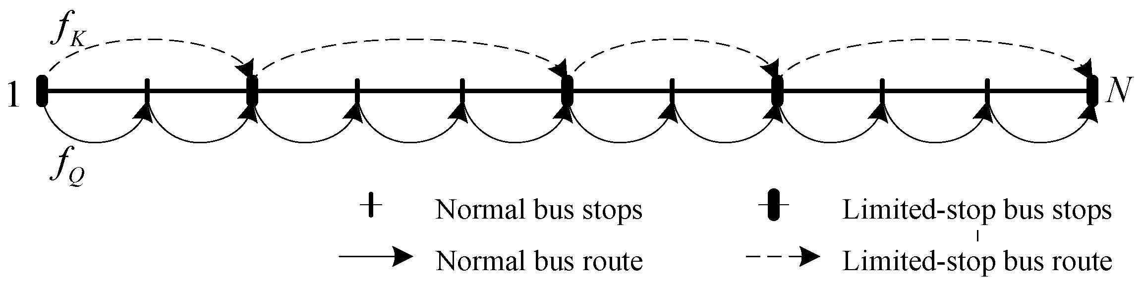
The proposed model is based on an isolated transit route with N stops. The trip demand is assumed to be fixed and known, and it is defined by an exogenous origin-destination (O-D) matrix of trips between stops that must be satisfied. The normal bus visits all stops, and f′_Q is the frequency of normal service of single scheduling per hour. The limited-stop bus visits only a subset of the stops on a route; f_Q and f_K are the frequency of normal service and limited-stop service of mixed scheduling, respectively. The mixed schedule of normal service and limited-stop service is illustrated in Figure 1.

The trip demand is assumed to be constant and known. The arrival of passengers at the bus stop is considered to be uniform. The waiting time that passengers are willing to bear is not long. The trip time for each passenger is assumed to be identical, and all buses drive at the same average speed. No bus is allowed to overtake and skip stops. The following section only shows the calculation of one direction, and the calculation of the other direction is identical.

2.2. Total Costs of a Bus Route

The benefits discussed in this paper are in terms of saving and better fleet utilization for the operators and travel time savings for the passengers. The use of a limited-stop bus service that serves only a subset of stops along certain routes appears to be a promising alternative given the benefits that they offer to both passengers and operators. For passengers, the limited-stop service implies improved service levels in the form of lower travel times due to fewer stops and higher between-stop speeds; for system operators, they enable demands to be met with fewer vehicles due to the shorter bus cycles.

The total costs include the passengers’ costs and bus operation cost. The passengers’ costs consist of the cost of access time, waiting time, and in-vehicle travel time as follows.

2.2.1. Access Time Cost

The access time cost includes two sections, one is the time elapsed from the moment a passenger begins a journey to the moment of arrival at the origin stop, another is the time elapsed between disembarking at the destination stop and arriving at the final destination. Since the origin and destination stop access times are assumed fixed for any trip, and the O-D matrix is fixed, the access time cost is constant and can be excluded from the objective function.

2.2.2. Waiting Time Cost

The waiting time cost reflects the time that passengers spend waiting at bus stops, which depends on the interval between consecutive vehicles. If the frequency of operation is f, then assuming that the passengers arrive uniformly at stops. The average passenger waiting time is often modelled as TE = k/f, where k depends on the distribution of bus arrival times at the stops. In systems with zero variability (that is, deterministic arrival times), the parameter takes the value of 0.5. However, bus arrivals are generally random, and if they are assumed to be Poisson-distributed, k is equal to 1 [13]. The following is expressions for single scheduling and mixed scheduling, respectively.

(1) Single scheduling

The waiting time cost of single scheduling, CWT₀ is expressed as Equation (1).

$$CW{T}_{{}^0}=\frac{60k{c}_w}{f_Q^{\prime }}{\displaystyle \sum _{i=1}^{N-1}{\displaystyle \sum _{j=i+1}^N{q}_{ij}}}$$

(1)

where c_w is the waiting time for a passenger. q_ij is the passenger OD, i = 1, 2, …, N − 1, j = 1, 2, …, N, which means boarding stop and alighting stop, respectively.

(2) Mixed scheduling

The waiting time cost of mixed scheduling can be divided into two components, namely the passengers’ cost at the normal stops and passengers’ cost at the limited stops. The waiting time cost of mixed scheduling, CWT can be modelled as following, in Equation (2).

$$CW{T}_{}=CW{T}_k+CW{T}_q =k{c}_w\left[\frac{60}{f_K}{\displaystyle \sum _{i=1}^{N-1}{\displaystyle \sum _{j=i+1}^N{\theta }_i{\theta }_j{q}_{ij}}}+\frac{60}{f_Q}({\displaystyle \sum _{i=1}^{N-1}{\displaystyle \sum _{j=i+1}^N{q}_{ij}}}-{\displaystyle \sum _{i=1}^{N-1}{\displaystyle \sum _{j=i+1}^N{\theta }_i{\theta }_j{q}_{ij}})}\right]$$

(2)

where CWT_k and CWT_q are the waiting time cost of the limited-stop service and normal service, respectively. θ_i is a binary variable that indicates the service type at stop I, which is equal to 1 if the limited-stop service is offered and 0 if it is not, similarly for θ_j and θ_m.

2.2.3. In-Vehicle Travel Time Cost

The total in-vehicle travel time includes four components, namely, the total travel time with an average speed between stops, additional time taken due to acceleration and deceleration at the intermediate stops, T_a, drivers’ reaction time T_f, and total stopping time for boarding and alighting at various intermediate stops, which is determined by the longer time of boarding and alighting.

(1) Single scheduling

The in-vehicle travel time cost of single scheduling, CIV₀ can be expressed, as in Equation (3).

$$\begin{gathered} CI{V}_{{}_0}^{}=c_p\left\{{\displaystyle \sum _{i=1}^{N-1}{\displaystyle \sum _{j=i+1}^N{q}_{{}_{ij}}^{}}}{\displaystyle \sum _{i=1}^j{t}_{{}_{si}}^{}}+{\displaystyle \sum _{m=2}^{N-1}\left[\left(T_a+T_f+\frac{\max (B_{{}_{0m}}^{}{t}_b,A_{{}_{0m}}^{}{t}_a)}{f_Q^{\prime }}\right){\displaystyle \sum _{i=1}^{m-1}{\displaystyle \sum _{j=m+1}^N{q}_{{}_{ij}}^{}}}\right]}\right\}, \\ {B}_{0m}={\displaystyle \sum _{j=m+1}^N{q}_{mj}},A_{0m}={\displaystyle \sum _{i=1}^{m-1}{q}_{im}} \end{gathered}$$

(3)

where c_p is the travel time for a passenger. t_si is the average travel time between bus stops i and i + 1. B_0m is the number of boarding persons at the entering door at stop m. A_0m is the number of alighting persons at the alighting door at stop m. t_b and t_a are the boarding and alighting time per person, respectively.

(2) Mixed scheduling

The passengers that take the limited-stop bus must wait for the passengers boarding and alighting at the non-destination stops. The passengers that take the normal bus must wait for the passengers boarding and alighting at the non-destination stops. Thus, the total stopping time for boarding and alighting at various intermediate stops is made up of the above two components of stopping time.

The passengers that take the limited-stop bus must wait for the passengers boarding and alighting at the non-destination stops, and then this stopping time cost in vehicle, CIV_pk can be modelled as follows, in Equation (4).

$$\begin{gathered} CI{V}_{pk}=c_p{\displaystyle \sum _{m=2}^{N-1}\left[\left({\theta }_m{T}_a+{\theta }_m{T}_f+\frac{\max (t_b{B}_{Km},t_a{A}_{Km})}{f_K}\right){\displaystyle \sum _{i=1}^{m-1}{\displaystyle \sum _{j=m+1}^N{\theta }_i{\theta }_j{q}_{ij}}}\right]}, \\ {B}_{Km}={\displaystyle \sum _{j=m+1}^N{\theta }_m{\theta }_j{q}_{mj}},A_{Km}={\displaystyle \sum _{i=1}^{m-1}{\theta }_i{\theta }_m{q}_{im}} \end{gathered}$$

(4)

where B_km and A_km are the number of passengers boarding and alighting, respectively, at the limited stop m for limited-stop service of this mixed scheduling case.

The passengers that take the normal bus must wait for the passengers boarding and alighting at the non-destination stops, and then this stopping time cost in vehicle, CIV_pq is expressed as Equation (5).

$$CI{V}_{pq}=c_p{\displaystyle \sum _{m=2}^{N-1}\left[\left(T_a+T_f+\frac{\max \left(t_b\left(B_{0m}-B_{Km}\right),t_a\left(A_{0m}-A_{Km}\right)\right)}{f_Q}\right)\left({\displaystyle \sum _{i=1}^{m-1}{\displaystyle \sum _{j=m+1}^N{q}_{ij}}}-{\displaystyle \sum _{i=1}^{m-1}{\displaystyle \sum _{j=m+1}^N{\theta }_i{\theta }_j{q}_{ij}}}\right)\right]}$$

(5)

Thus, the total in-vehicle time cost of mixed scheduling, CIV is expressed as in Equation (6).

$$CIV=c_p\left\{\begin{array}{l}{\displaystyle \sum _{i=1}^{N-1}{\displaystyle \sum _{j=i+1}^N{q}_{ij}}}{\displaystyle \sum _{i=1}^j{t}_{si}}+{\displaystyle \sum _{m=2}^{N-1}\left[\left({\theta }_m{T}_a+{\theta }_m{T}_f+\frac{\max (t_b{B}_{Km},t_a{A}_{Km})}{f_K}\right){\displaystyle \sum _{i=1}^{m-1}{\displaystyle \sum _{j=m+1}^N{\theta }_i{\theta }_j{q}_{ij}}}\right]}\\ +{\displaystyle \sum _{m=2}^{N-1}\left[\left(T_a+T_f+\frac{\max \left(t_b\left(B_{0m}-B_{Km}\right),t_a\left(A_{0m}-A_{Km}\right)\right)}{f_Q}\right)\left({\displaystyle \sum _{i=1}^{m-1}{\displaystyle \sum _{j=m+1}^N{q}_{ij}}}-{\displaystyle \sum _{i=1}^{m-1}{\displaystyle \sum _{j=m+1}^N{\theta }_i{\theta }_j{q}_{ij}}}\right)\right]}\end{array}\right\}$$

(6)

2.2.4. Operation Cost

The operation cost can be decomposed into fixed costs, variable costs. The fixed costs include all costs that do not depend on the number of buses in circulation, such as the operator’s management and general administrative expenses. The variable costs include distance-based and time-dependent variable costs. The variable costs that depend on the distance travelled can be expressed as the cost per vehicle-kilometre and is generally a function of the physical characteristics of the route served, such as the number of stops, route grade, and operation factors such as the vehicle speeds and accelerations between stops [10]. The variable operation costs that depend on time include employment costs, bus acquisitions, taxes, licenses and insurance and can be measured on a per vehicle-hour basis [10]. This part of the variable costs can be expressed as the product of cost per hour and cycle time.

(1) Single scheduling

The operation cost of single scheduling, COP₀ is expressed as follows in Equation (7).

$$CO{P}_0=c_s{f}_Q^{\prime }L+c_t{f}_Q^{\prime }{T}_Q^{\prime } =c_s{f}_Q^{\prime }L+c_t{f}_Q^{\prime }\left[{\displaystyle \sum _{i=1}^{N-1}{t}_{si}}+{\displaystyle \sum _{m=2}^{N-1}\left(T_a+T_f+\frac{\max (t_b{B}_{0m},t_a{A}_{0m})}{f_Q^{\prime }}\right)}\right]$$

(7)

where c_s and c_t are the operation cost per vehicle-hour and operation cost per vehicle-kilometre, respectively. T’_Q is the cycle time of single scheduling.

(2) Mixed scheduling

The operation cost of mixed scheduling, COP is expressed as follows in Equation (8).

$$\begin{array}{l}COP=c_s(f_Q+f_K)L+c_t{f}_Q{T}_Q+c_t{f}_K{T}_K\\ \hspace{1em} =c_s(f_Q+f_K)L+c_t{f}_Q\left\{{\displaystyle \sum _{i=1}^{N-1}{t}_{si}}+{\displaystyle \sum _{m=2}^{N-1}\left[\left(T_a+T_f+\frac{\max \left(t_b\left(B_{0m}-B_{Km}\right),t_a\left(A_{0m}-A_{Km}\right)\right)}{f_Q}\right)\right]}\right\}\\ \hspace{1em}\hspace{1em}+c_t{f}_K\left\{{\displaystyle \sum _{i=1}^{N-1}{t}_{si}}+{\displaystyle \sum _{m=2}^{N-1}\left[\left({\theta }_m{T}_a+{\theta }_m{T}_f+\frac{\max (t_b{B}_{Km},t_a{A}_{Km})}{f_K}\right)\right]}\right\}\end{array}$$

(8)

where T_Q and T_K are the cycle time of the normal bus and limited-stop bus, respectively.

The above analysis only addresses the inbound trips, and it is identical to the analysis of outbound trips. It is necessary to sum both inbound trips and outbound trips to analyse the scheduling.

2.3. Objective Function

A multi-objective optimization problem is commonly converted to a single-objective model in the literature. The multi-objective function for this model is the sum of the waiting time cost, in-vehicle travel time cost and operation cost.

(1) Single scheduling

The total cost of single scheduling, CS₀ is the sum of Equations (1), (3) and (7) of both inbound and outbound trips, and is expressed as follows in Equation (9).

$$Min C{S}_0(f_Q^{\prime })=w_p\left(CW{T}_0+CI{V}_0\right)+w_{o}CO{P}_0$$

(9)

where w_p and w_o are the non-negative weights, which can be adjusted for different bus routes with different passenger demands.

(2) Mixed scheduling

The total cost of mixed scheduling, CS is the sum of Equations (2), (6) and (8) of both inbound and outbound trips, and is expressed as follows in Equation (10).

$$Min CS(f_Q,f_K)=w_p\left(CW{T}_{}+CI{V}_{}\right)+w_{o}CO{P}_{}$$

(10)

$$s.t.F=F_g$$

(11)

$$f_{\min }\le f\le f_{\max }$$

(12)

$${\alpha }_{\min }\le \alpha \le {\alpha }_{\max }$$

(13)

where, the constraint of Equation (11) ensures that the fleet size F is F_g. The fleet size F is the product of frequency and cycle time. F_g is the fleet size limitation. The constraint of Equations (12) and (13) ensure the value of frequency f and load factor α. Here, $f=\{\begin{array}{l}{f}_Q^{\prime }, \hspace{1em}{\theta }_i=0\\ f_Q+f_K,{\theta }_i=1\end{array}$. The load factors of the normal bus in single scheduling, α₀, normal bus in mixed scheduling, α_q, and limited-stop bus in mixed scheduling, α_k are expressed as Equations (14)–(16), respectively.

$${\alpha }_0=\frac{\underset{m=2,3,\dots ,N-1}{\max }{\displaystyle \sum _{i=1}^m{\displaystyle \sum _{j=m+1}^N{q}_{ij}}}}{f_Q^{\prime }\times PL}\times 100\%$$

(14)

$${\alpha }_q=\frac{\underset{m=2,3,\dots ,N-1}{\max }\left({\displaystyle \sum _{i=1}^m{\displaystyle \sum _{j=m+1}^N{q}_{ij}}}-{\displaystyle \sum _{i=1}^{m-1}{\displaystyle \sum _{j=m+1}^N{\theta }_m{\theta }_i{\theta }_j{q}_{ij}}}\right)}{f_Q\times PL}\times 100\%$$

(15)

$${\alpha }_k=\frac{\underset{m=2,3,\dots ,N-1}{\max }{\displaystyle \sum _{i=1}^m{\displaystyle \sum _{j=m+1}^N{\theta }_m{\theta }_i{\theta }_j{q}_{ij}}}}{f_K\times PL}\times 100\%$$

(16)

where PL is the vehicle capacity.

2.4. Solution Algorithm

This model is used to analyze two parts of the contents. The first part discusses the changes of the frequencies, fleets and costs of optimal decision with constraints of different load factor. Here, constraint conditions ($f_{\min }\le f\le f_{\max }$) and (${\alpha }_{\min }\le \alpha \le {\alpha }_{\max }$) are only considered, but constraint condition ($F\le F_g$) is not considered. The second part is a comparative analysis of the optimization solution with the constraint of different fleet size, where constraint ($F\le F_g$) is taken into account.

For the single scheduling, the optimization of frequency can be calculated by the first derivation. However, for the mixed scheduling, the proposed minimization model is a mixed nonlinear integer programming model. The objective function is not convex or concave, which is an NP-hard problem and difficult to solve using any exact algorithm. The heuristic algorithm has a good effect on coping with this problem. There are many different domains where metaheuristics and nature-inspired algorithms have been applied as solution approaches, such as online learning, intermodal terminal operations, multi-objective optimization, vehicle routing, medicine, data classification, and others [30,31,32,33,34]. A genetic algorithm could be used to yield a minimum-cost transit operation for optimizing bus frequencies and transit routes and [18,22,35,36]. Genetic algorithms can efficiently cope with mixed-integer non-linear problems and the objective function gradient does not require calculation, thus reducing computational effort.

In solving the model, the genetic algorithm is used to implement genetic operation on individuals in the population based on the objective function. The first step of applying genetic algorithm to solve the optimization of bus frequency is to express the gene of bus frequency, as the decision variable is the bus frequency. f_Q and f_K are the frequency of normal service and limited-stop service of mixed scheduling, respectively, and they are encoded as [f_Q, f_K] by using two-dimensional real number. f′_Q is the frequency of normal service of single scheduling per hour. In the iterative process, individuals of the population are optimized generation by generation and gradually approach the optimal solution. The specific steps of this solution method are as follows:

Step 1: Initiate the frequency (f_Q, f_K and f′_Q). Randomly generate N individuals as initial population P₍₀₎. Set the number of iterations, and the maximum number of iterations for the genetic algorithm as T, and set the number of elites and the crossover probability. Individuals in the initial population are randomly generated. In order to generate the optimization of the first part, the constraint conditions are ($f_{\min }\le f\le f_{\max }$) and (${\alpha }_{\min }\le \alpha \le {\alpha }_{\max }$). In order to generate the optimization of the second part, the constraint condition ($F\le F_g$) needs to be added.

Step 2: Calculate the value of the objective function, according to Equation (10). Because the objective function is formed to minimize cost, the objective function is equal to the reciprocal of the fitness function.

Step 3: The selection, crossover, and mutation of chromosomes are applied to produce new chromosomes.

Step 4: The termination condition is given the maximum number of iterations. If t = T, the individual with the maximum fitness obtained in the evolution process is output as the optimal solution and the calculation is terminated. Otherwise, go to Step 3.

2.5. Data and Parameter Setting

We took a bus route in Zhenjiang city of China as an example to verify the validity of the proposed model. Bus route 202 connects Zhenjiang railway station and Rongbing town. It is 46 kilometres long with 32 bus stops in total. The demand of boarding/alighting passengers at each stop during the morning peak was investigated and shown in

Table 1. OD matrix of Bus Route 202 in the direction of Rongbing → Zhenjiang railway station during the morning peak (7:00 a.m.–8:00 a.m.).

O-D	Passenger Demand	O-D	Passenger Demand	O-D	Passenger Demand	O-D	Passenger Demand
1–7	20	1–8	20	1–10	20	1–11	20
1–15	20	1–23	22	1–26	12	1–31	20
1–32	8	2–11	20	2–15	20	2–31	16
2–32	24	3–32	16	4–11	20	4–15	20
4–26	20	4–31	24	5–30	20	5–32	20
6–31	20	7–31	24	7–32	16	8–23	16
8–26	24	8–29	28	8–31	12	8–32	24
9–19	24	9–23	36	9–26	24	9–29	20
9–31	20	10–23	24	10–30	16	10–32	20
11–30	20	11–32	20	12–31	20	12–32	20
13–31	20	14–32	20	15–20	16	15–22	20
15–23	48	15–24	24	15–32	92	15–32	28
16–23	12	16–28	20	16–31	28	16–32	12
17–32	20	18–30	20	18–32	20	19–27	16
19–31	44	19–32	20	20–28	12	20–31	16
20–32	24	21–32	20	23–32	20	24–32	24
25–32	52

and Figure 2. All other OD pairs that are not shown in this table have zero demand.

As seen from Figure 2, the passengers flow boarding/alighting at Stops #2, 4, 8, 9, 10, 11, 15, 16, 19, 20, 23, 26, 30, and 31 were obviously more than those at other stops. As shown in the Table 1, the OD pair number between these eleven intermediate stops was 514 person times, and the number of all OD pairs was 770 person times. Therefore, these eleven intermediate stops were confirmed as the limited stops. The arrival of buses at the various stops was assumed as deterministic. Because the maximum demand of boarding/alighting person was 514 person times per hour, the maximum and minimum frequencies were set as 20 and 2 times per hour respectively. Here, k is 0.5; t_s is 2.2 min; t_b is 2 s; t_a is 1.5 s; T_a is 30 s; T_f is 12 s; c_w is 0.7 $/min; c_p is 0.5 $/min; c_s is 7 $/km∙veh; c_t is 3.5 $/min∙veh; PL is 75. Because the passengers’ cost should be higher, we set the weight w_p as 0.6, and w_o as 0.4.

3. Results and Discussion

3.1. Results

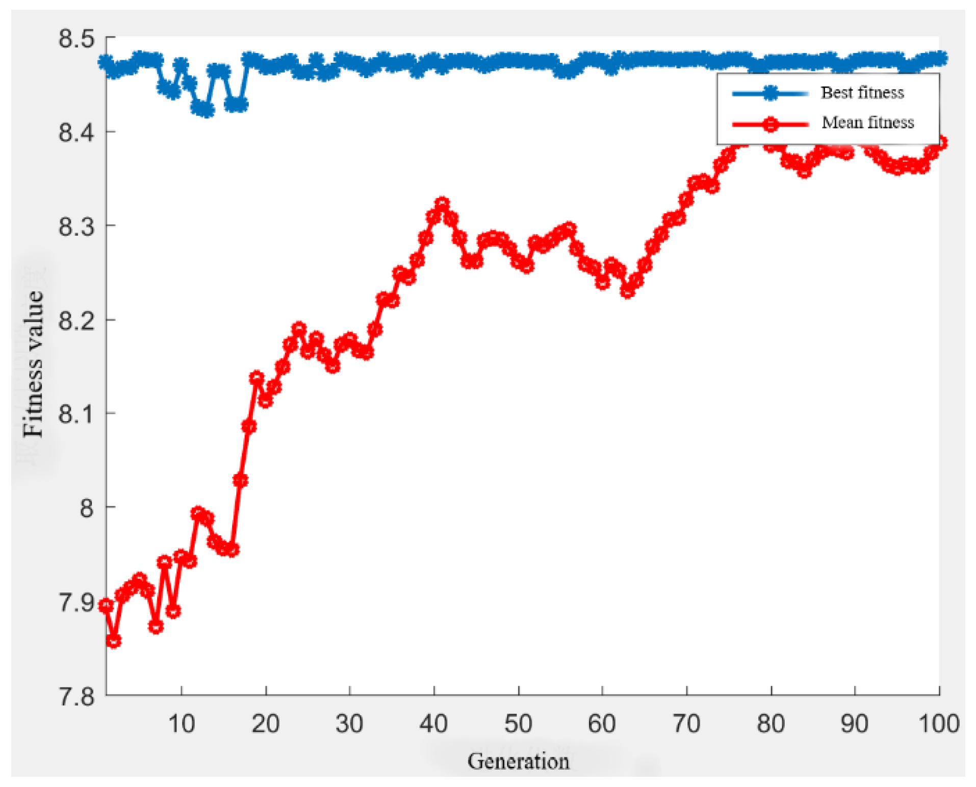
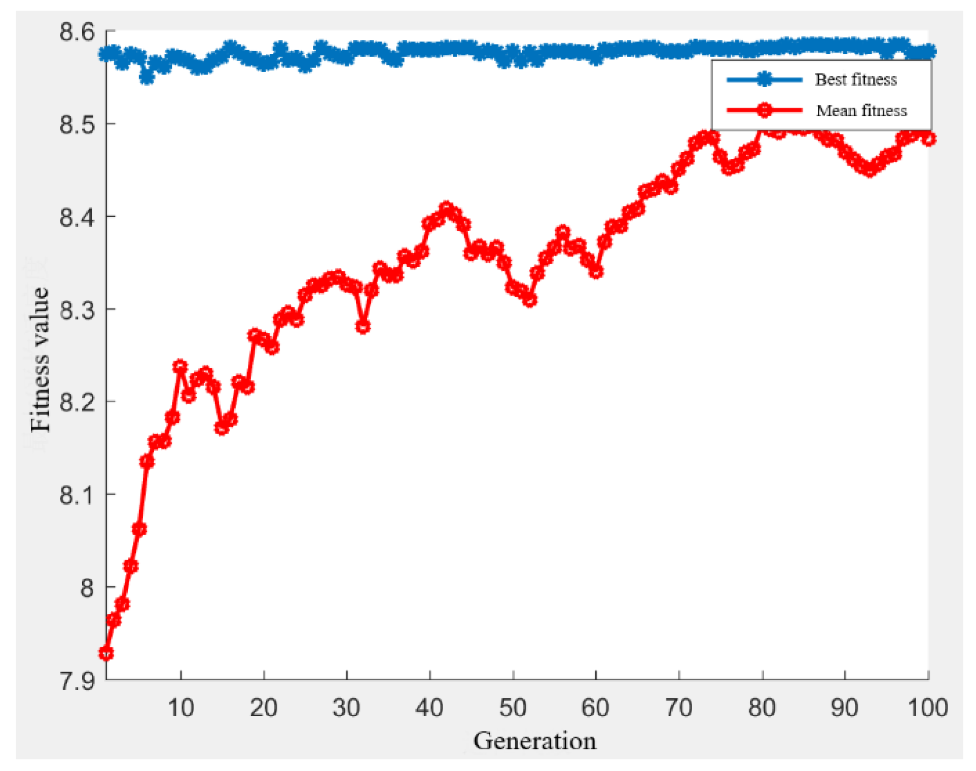
A genetic algorithm was used to solve this multi-object model. This algorithm was calculated by the “Genetic Algorithm and Direct Search Toolbox” by MATLAB 2012(b) and implemented on a personal computer with Intel Core i5-3470 CPU @ 3.20 GHz, 3.20 GHz and 4.00 GB RAM. We randomly generated 100 individuals as the initial population and set the maxim generation numbers as 100 and crossover fraction as 0.09. A convergence trend of the solution algorithm for single scheduling model and mixed scheduling model are observed in Figure 3 and Figure 4, respectively.

3.2. Discussion

3.2.1. Sensitivity Analysis of Different Load Factors

The following discussed the variation of frequency, fleet size, and cost for different load factor constraints.

Table 2. Frequencies, fleet size and costs of different load factor constraints.

αmin~αmax (%)	Schedule Type	α (%)		f (buses/h)		F (buses)		Cycle Time (min)		Wait Time Cost ($)	In-Vehicle Time Cost ($)	Operation Cost ($)	Total Cost ($)	△CS (%)
		I	II	I	II	I	II	I	II
50~90	Single	61.6		13.3		50		197		1742	178,272	17,670	197,686	−3.1
	Mixed	90	50	8.8	2	30	6	199	174	3740	173,502	14,246	191,488
50~100	Single	61.6		13.3		50		197		1742	178,272	17,670	197,686	−4.4
	Mixed	100	50	8.2	2.6	28	8	199	174	3804	171,064	14,200	189,068
50~120	Single	61.6		13.3		50		197		1742	178,272	17670	197,686	−7.1
	Mixed	120	50	6.8	4	24	12	199	174	3992	165,656	14,094	185,176

I: normal bus; II: limited-stop bus. △CS(%): the percentage increase of mixed schedule to single schedule of total cost.

listed the frequencies, fleets and costs of optimal decision generated by the model with constraints of different load factor. Here, the minimum load factor was set as 50%, and the maximum load factors were set as 90%, 100% and 120% respectively. The three load factor constraints were set as 50–90%, 50–100%, and 50–100%. The following is a comparative analysis of the optimal scheduling scheme for normal bus and limited-stop bus under these three load factor constraints. We compared the cost differences of actually load factor, departure frequency, fleet size, cycle time, wait time cost, in-vehicle time cost, operation cost and total cost. In addition, we also compared the cost variation of the optimal solution under combined versus single dispatch.

Under the single scheduling, regardless of whether the upper limit constraint on load factor increases or decreases, the optimal solution was unchanged with a frequency of 13.3 buses per hour, an actual load factor of 61.6%, a fleet size of 50, a cycle time of 197 min, and a constant total cost.

Under the mixed scheduling, there were three different optimal scenarios of the three load factor constraints. As the maximum load factor constraint was increased, the frequency of departures for normal bus service decreased from 8.8 to 6.8, the load factor increased from 90% to 120%, and the fleet size decreased from 30 to 24. The frequency of limited-stop bus service was increased from two to four, the load factor was maintained at 50%, and the fleet size was increased from six to twelve. The total fleet size remained unchanged at 36 vehicles. When the fleet size was more than 36, the load factors were lower than 50%. It could be found that both frequencies and fleets of the normal bus were clearly reduced when the upper limit of the load factor increases from 90% to 120%. When the load factor constraint was activated, these services tend to be replaced with higher frequencies on limited-stop services. The total cost of the mixed scheduling decreased with increasing load factor. The waiting time cost increased because of the lower frequencies of normal buses. Because of the higher frequencies and less in-vehicle time of limited-stop buses, the in-vehicle time cost and operation cost decreased. The in-vehicle time cost shared most of the total cost, and the total cost was reduced.

Comparing the costs of single scheduling and mixed scheduling, several changes can be observed. Under the same load factor constraint, the in-vehicle time cost, operation cost and total cost of mixed scheduling were much lower than the single scheduling. Only wait time cost was higher than the single scheduling.

3.2.2. Sensitivity Analysis of Different Fleet Sizes

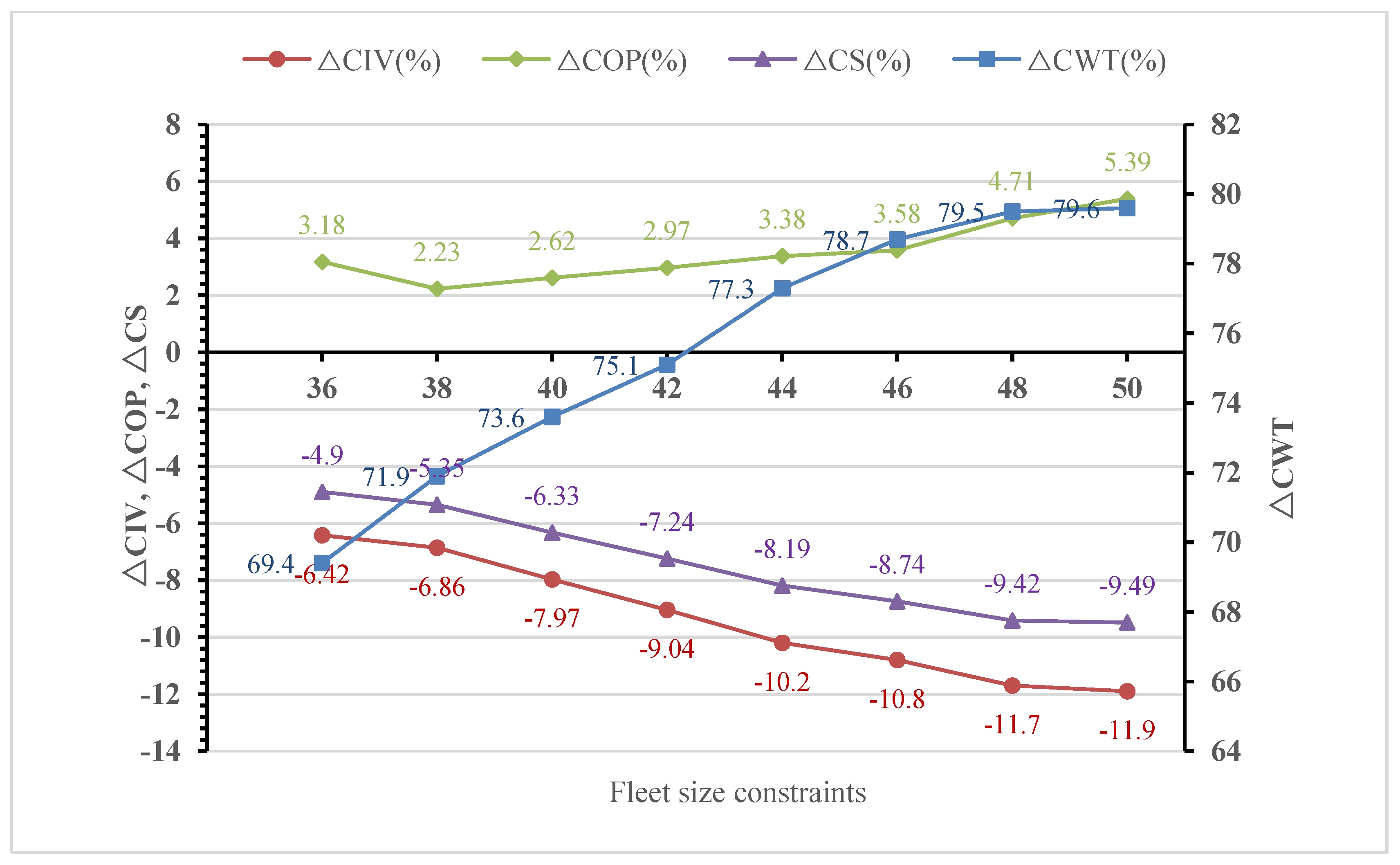
Considering passenger comfort, we set 100% as an upper bound on the full load factor. Under this load factor constraint, the capacity size of the optimal solution was 25 and 18 for single scheduling and mixed scheduling, respectively. We further compared and analyzed the optimal solution with the constraint of different fleet size, and the results are shown in

Table 3. Frequencies, fleet of different fleet size constraints.

Fg (buses)	Type of Schedule	f (buses/h)		A (%)		F (buses)		Cycle Time (min)
		I	II	I	II	I	II	I	II
36	Single	10.3		80		36		198
	Mixed	8.2	2.6	100	50	28	8	199	174
38	Single	10.9		75.2		38		198
	Mixed	8.31	2.97	98	48	30	8	198	173
40	Single	11.1		71		40		198
	Mixed	8.3	3.6	98	45	30	10	198	173
42	Single	12		62		42		197
	Mixed	8.27	4.35	99	43	30	12	198	173
44	Single	12.6		65		44		197
	Mixed	8.16	5.14	100	40	28	16	198	173
46	Single	13.1		62		46		197
	Mixed	8.22	5.74	99	39	28	18	198	173
48	Single	13.7		60		48		197
	Mixed	8.16	6.48	100	37	28	20	198	173
50	Single	14.1		62		50		197
	Mixed	8.2	7.2	100	35	28	22	198	172

and Figure 5.

As seen from Table 3 and Figure 5, with the increase in fleet size, the load factor, cycle time, waiting time cost and in-vehicle time cost decreased, and only the operation costs increased. Finally, the total costs were still reduced.

The objective function values of different scheduling types are compared. Compared with the single scheduling case, the passengers’ waiting time cost and in-vehicle time cost reduce because of the limited-stop service. The operation cost always increases because of the higher frequency, and the increased operation cost is $c_{s}L(f_Q^{}+f_K-f_Q^{\prime })$. However, the total cost decreases under mixed scheduling.

The result of the application of this model to Bus Route 202 is that the inclusion of the limited-stop service achieved a savings of 9.49% compared to the single scheduling service. When the fleet size increases from 36 to 50, the cost saving tends to increase from 4.9% to 9.49%. When the fleet size is smaller, the frequency of limited-stop buses is less than two times per hour. However, it is difficult to make full use of the advantages of limited-stop buses, and the passengers’ trip time costs will increase. Therefore, single scheduling is better than mixed scheduling when the fleet size is smaller.

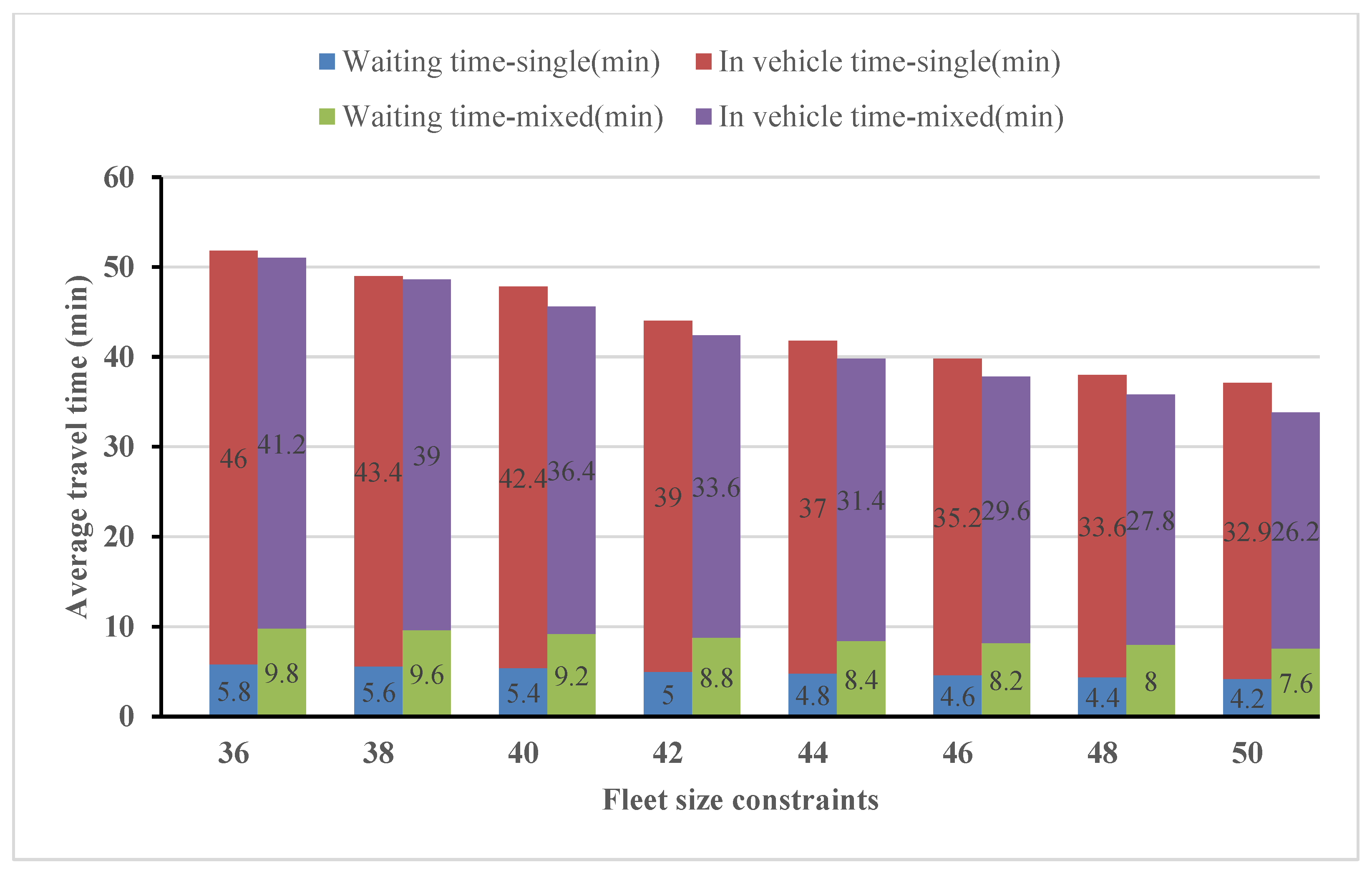
3.2.3. Analysis of the Travel Time Saving

Figure 6 compares the average travel time of different scheduling types.

When the fleet size increases from 36 to 50, the passengers’ waiting time, in-vehicle time and total travel time decrease. Under the same fleet size, the passengers’ waiting time increases, but the in-vehicle time and total travel time are less than those under the single scheduling service. For example, when the fleet size is 44, the waiting time and in-vehicle time are 77.3% higher and 15.1% lower than those under single scheduling, respectively. The total travel time of limited-stop services achieves a saving of 4.5% compared to that of the single scheduling service, which is a normal service that visits every stop on a line at its optimal frequency. The optimal results are also obvious when the fleet size is growing.

4. Conclusions

This paper has presented an optimization method to design a limited-stop transit service that minimizes the total cost. Since the method was intended to be used in a known trip matrix, the minimization problem was equivalent to minimize the cost, that is, both bus system operating cost and the costs in terms of the waiting time, in-vehicle travel time, etc. A numerical example of Bus Route 202 was used to testify the feasibility of the proposed methodology. A genetic algorithm was used to calculate the mixed dispatching frequency scheme of limited-stop and normal-bus service. The results are compared with those of single scheduling. Moreover, a sensitivity analysis is conducted to further investigate the impacts of the demand on the load factor and fleet size. The discussion results are summarized as follows.

(1)

The cycle time of limited-stop service achieved a savings of 5.76% compared to that of single scheduling: a normal-service visiting every stop on a line at its optimal frequency.

(2)

When the load factor constraint is activated, these services tend to be replaced with higher frequencies on limited-stop services, and the total cost of the mixed scheduling service decreases with the increasing load factor.

(3)

Under the same load factor constraint, the total cost is lower when the system is operated under the mixed scheduling service compared to that under the single scheduling service.

(4)

Under the same fleet size constraint, the passenger travel time and operation cost obtained by offering the limited-stop services are significant savings, especially when the fleet size increases.

In general, this study contributed to the depth analysis of the relationship among the influencing factors of mixed scheduling, such as departure interval, fleet size and cost by combining the passenger flow and the capacity limitation. However, some shortcomings remain. The model established here is suitable for bus routes with imbalanced passenger flow sections and long-distance travel needs. When the bus passenger flow presents such characteristics, the advantages of limited-stop bus service are prominent. The demand variability among different O-D pairs is an important factor in the design of limited-stop service, and the analysis should test the effects of different characteristics of the demand profile. The analysis presented here can also be extended from an isolated transit route to a more complete transit system such as a corridor. In the construction of this multi-objective model, the following two aspects have not been fully considered: one is the behaviour of passengers’ individual choice; the other is the benefits brought by the mixed scheduling service to the operation of bus companies. Further research will make up for the above deficiencies.

References

- Liang, M.; Zhang, H.M.; Ma, R.; Wang, W.; Dong, C. Cooperatively coevolutionary optimization design of limited-stop services and operating frequencies for transit networks. Transp. Res. Part C Emerg. Technol. 2021, 125, 103038. [Google Scholar] [CrossRef]
- Suman, H.; Larrain, H.; Muñoz, J.C. The impact of using a naïve approach in the limited-stop bus service design problem. Transp. Res. Part A Policy Pract. 2021, 149, 45–61. [Google Scholar] [CrossRef]
- Tang, C.Y.; Ceder, A.; Zhao, S.C. Minimizing User and Operator Costs of Single Line Bus Service Using Operational Strategies. Transport 2018, 33, 993–1004. [Google Scholar] [CrossRef] [Green Version]
- Zhang, H.; Zhao, S.Z.; Cao, Y.; Liu, H.S.; Liang, S.D. Real-Time Integrated Limited-Stop and Short-Turning Bus Control with Stochastic Travel Time. J. Adv. Transp. 2017, 2017, 2960728. [Google Scholar] [CrossRef] [Green Version]
- Tang, C.Y.; Ceder, A.; Zhao, S.C.; Ge, Y.E. Determining Optimal Strategies for Single-Line Bus Operation by Means of Smartphone Demand Data. Transp. Res. Rec. 2006, 2539, 130–139. [Google Scholar] [CrossRef]
- Clarens, G.C.; Hurdle, V.F. An operating strategy for a commuter bus system. Transp. Sci. 1975, 9, 1–20. [Google Scholar] [CrossRef]
- Abkowitz, M.; Engelstein, I. Methods for maintaining transit service regularity. Transp. Res. Rec. 1984, 1961, 1–8. [Google Scholar]
- Furth, P.G.; Day, B. Transit routing and scheduling strategies for heavy demand corridors. Transp. Res. Rec. 1985, 1011, 23–26. [Google Scholar]
- Vijayaraghavan, T.A.S. Fleet Assignment strategies in urban transportation using express and partial services. Transp. Res. Part A 1995, 29, 157–171. [Google Scholar] [CrossRef]
- Vuchic, V.R. Urban. Transit. Operations, Planning and Economics; John Wiley and Sons: Indianapolis, IN, USA, 2005. [Google Scholar]
- El-Geneidy, A.M.; Surprenant-Legault, J. Limited-stop bus service: An evaluation of an implementation strategy. Public Transp. 2010, 2, 291–306. [Google Scholar] [CrossRef]
- Stacey, S.; Sarah, W. Intermediate time point removal on limited-stop routes at New York city transit. In Proceedings of the 92th Annual Meeting of the Transportation Research Board, Washington, DC, USA, 13–17 January 2013. [Google Scholar]
- Ceder, A. Designing public transport network and routes. In Advanced Modeling for Transit Operations and Service Planning; Emerald Group Publishing Limited: Bradford, UK, 2003; pp. 59–92. [Google Scholar]
- Barnhart, C.; Laporte, G. Handbooks in Operations Research and Management Science: Transportation; Elsevier: Amsterdam, The netherlands, 2006. [Google Scholar]
- Guihaire, V.; Hao, J.K. Transit network design and scheduling: A global review. Transp. Res. Part A Policy Pract. 2008, 42, 1251–1273. [Google Scholar] [CrossRef] [Green Version]
- Leiva, C.; Muñoz, J.C.; Giesen, R.; Larrain, H. Design of limited-stop services for an urban bus corridor with capacity constraints. Transp. Res. Part B Methodol. 2010, 44, 1186–1201. [Google Scholar] [CrossRef]
- Tetreault, P.R.; El-Geneidy, A.M. Estimating bus run times for new limited-stop service using archived AVL and APC data. Transp. Res. Part A Policy Pract. 2010, 44, 390–402. [Google Scholar] [CrossRef]
- Niu, H. Determination of the skip-stop scheduling for a congested transit line by bilevel genetic algorithm. Int. J. Comput. Intell. Syst. 2011, 4, 1158–1167. [Google Scholar]
- Liu, Z.Y.; Yan, Y.D.; Qu, X.; Zhang, Y. Bus stop-skipping scheme with random travel time. Transp. Res. Part C Emerg. Technol. 2013, 35, 46–56. [Google Scholar] [CrossRef]
- Chen, J.X.; Liu, Z.Y.; Zhu, S.L.; Wang, W. Design of limited-stop bus service with capacity constraint and stochastic travel time. Transp. Res. Part E Logist. Transp. Rev. 2015, 83, 1–15. [Google Scholar] [CrossRef]
- Maxime, F.; Giesen, R.; Muñoz, J.C. Continuous approximation for skip-stop operation in rail transit. Transp. Res. Part C Emerg. Technol. 2013, 36, 419–433. [Google Scholar]
- Yi, Y.; Choi, K.; Lee, Y.J. Optimal Limited-stop Bus Routes Selection Using a Genetic Algorithm and Smart Card Data. J. Public Transp. 2016, 19, 178–198. [Google Scholar] [CrossRef] [Green Version]
- Zhang, H.; Zhao, S.Z.; Liu, H.S.; Liang, S.D. Design of limited-stop service based on the degree of unbalance of passenger demand. PLoS ONE 2018, 13, e0193855. [Google Scholar] [CrossRef] [Green Version]
- Torabi, M.; Salari, M. Limited-stop bus service: A strategy to reduce the unused capacity of a transit network. Swarm Evol. Comput. 2019, 44, 972–986. [Google Scholar] [CrossRef]
- Alam, A.; Diab, E.; El-Geneidy, A.M.; Hatzopoulou, M. A simulation of transit bus emissions along an urban corridor: Evaluating changes under various service improvement strategies. Transp. Res. Part D Transp. Environ. 2014, 31, 189–198. [Google Scholar] [CrossRef]
- Hart, N. Methodology for Evaluating Potential for Limited-Stop Bus Service along Existing Local Bus Corridors. Transp. Res. Rec. 2016, 2543, 91–100. [Google Scholar] [CrossRef]
- Soto, G.; Larrain, H.; Munoz, J.C. A new solution framework for the limited-stop bus service design problem. Transp. Res. Part B Methodol. 2017, 105, 67–85. [Google Scholar] [CrossRef]
- Zhang, H.; Liu, H.S.; Zhao, S.Z.; Liang, S.D. Optimising the design of a limited-stop bus service for a branching network. Proc. Inst. Civ. Eng. Munic. Eng. 2017, 170, 230–238. [Google Scholar] [CrossRef] [Green Version]
- Wang, D.Z.W.; Nayan, A.; Szeto, W.Y. Optimal bus service design with limited stop services in a travel corridor. Transp. Res. Part E Logist. Transp. Rev. 2018, 111, 70–86. [Google Scholar] [CrossRef]
- Zhao, H.; Zhang, C. An online-learning-based evolutionary many-objective algorithm. Inf. Sci. 2020, 509, 1–21. [Google Scholar] [CrossRef]
- Dulebenets, M.A. A Delayed Start Parallel Evolutionary Algorithm for just-in-time truck scheduling at a cross-docking facility. Int. J. Prod. Econ. 2019, 212, 236–258. [Google Scholar] [CrossRef]
- Liu, Z.Z.; Wang, Y.; Huang, P.Q. A many-objective evolutionary algorithm with angle-based selection and shift-based density estimation. Inf. Sci. 2020, 509, 400–419. [Google Scholar] [CrossRef] [Green Version]
- Pasha, J.; Dulebenets, M.A.; Kavoosi, M.; Abioye, O.F.; Wang, H.; Guo, W. An Optimization Model and Solution Algorithms for the Vehicle Routing Problem with a “Factory-in-a-Box”. IEEE Access 2020, 8, 134743–134763. [Google Scholar] [CrossRef]
- D’Angelo, G.; Pilla, R.; Tascini, C.; Rampone, S. A proposal for distinguishing between bacterial and viral meningitis using genetic programming and decision trees. Soft Comput. 2019, 23, 11775–11791. [Google Scholar] [CrossRef]
- Agrawal, J.; Mathew, T.V. Transit Route Network Design Using Parallel Genetic Algorithm. J. Comput. Civ. Eng. 2004, 18, 248–256. [Google Scholar] [CrossRef]
- Fan, W.; Machemehl, R.B. Optimal transit route network design problem with variable transit demand: Genetic algorithm approach. J. Transp. Eng. 2006, 132, 40–51. [Google Scholar] [CrossRef]
Figure 1.
Organization of the mixed schedule of normal service and limited-stop service.
Figure 2.
Passengers demand of boarding/alighting at the stop from Zhenjiang to Rongbing during the morning peak (7:00 a.m.~8:00 a.m.).
Figure 3.
Convergence trend of the solution algorithm for single scheduling model.
Figure 4.
Convergence trend of the solution algorithm for mixed scheduling model.
Figure 5.
The waiting time cost, in-vehicle time cost, operation cost and total cost of different fleet size constraints. △CWT(%), △CIV(%) and △COP(%) mean the percentage increase of mixed schedule to single schedule of waiting time cost, in-vehicle time cost, and operation cost, respectively.
Figure 6.
Average travel time of different scheduling types.