Analysis of Two-Worm Interaction Model in Heterogeneous M2M Network

Abstract

With the rapid development of M2M (Machine-to-Machine) networks, the damages caused by malicious worms are getting more and more serious. By considering the influences of the network heterogeneity on worm spreading, we are the first to study the complex interaction dynamics between benign worms and malicious worms in heterogeneous M2M network. We analyze and compare three worm propagation models based on different immunization schemes. By investigating the local stability of the worm-free equilibrium, we obtain the basic reproduction number R₀. Besides, by using suitable Lyapunov functions, we prove that the worm-free equilibrium is globally asymptotically stable if R₀ ≤ 1, otherwise unstable. The dynamics of worm models is completely determined by R₀. In the absence of birth, death and users’ treatment, we obtain the final size formula of worms. This study shows that the nodes with higher node degree are more susceptible to be infected than those with lower node degree. In addition, the effects of various immunization schemes are studied. Numerical simulations verify our theoretical results. The research results are meaningful for us to further understand the spread of worms in heterogeneous M2M network, and enact effectual control tactics.

1. Introduction

With the development of cloud computing and M2M technologies, the threat from worms and their variants is becoming increasingly serious. According to the 2015 Symantec Global Internet Security Threat Report [1], the year 2014 is a year with far-reaching vulnerabilities, faster attacks, files held for ransom, and far more malicious code than in previous years. Many measures are taken against the propagation of malicious worms, such as anti-virus software, patch, firewall, etc. However, those measures cannot understand the transmission mechanisms of worms, and cannot predict the spread trends of worms [2]. Thus, those general defense and detection measures cannot help us to provide more effective measures against malicious worms and their variants.

Mathematical modeling is an important tool in analyzing and controlling the spread of malicious worms. The process of model formulation comprehensively uses assumptions, parameters, and variables. Besides, those models provide us theoretical conclusions, such as basic reproduction rate, feasible region, effective contact rate, and thresholds. Theoretical analysis and numerical simulations are useful tools for testing theoretical results, determining how to change sensitive parameter values, getting key parameters according to known date, and establishing effective control measures. Mathematical models effectively help us understand the mechanisms of worm propagation, predict the spread trends of worm, and develop better approaches for decreasing the transmission of malicious worms.

According to network characteristics, networks can be divided into two kinds: homogeneous and heterogeneous networks. In a homogeneous network, most nodes have similar degrees, and nodes’ degree distribution is very similar; homogeneous networks include regular networks [3], Erdӧs-Renyi random networks [4], and small-world networks [5]. Many epidemic models [6,7,8,9,10,11,12,13,14,15] have been developed to understand the spreading dynamics based on the fully-connected assumption of the homogeneous network. In those models, whole nodes are divided into different compartments corresponding to different epidemiological states. Nevertheless, this fully-connected assumption is inconsistent with the real world network topology; that is, the assumption that each computer has an equal probability of scanning any other individual in the network is unreasonable. Thus, the homogeneous mixing hypothesis is an overly simplified assumption, and is generally unrealistic. It is not appropriate for modeling epidemic models in heterogeneous networks. Contrary to homogeneous networks, most nodes of heterogeneous network have large fluctuations in degree distribution; heterogeneous networks include scale-free networks [16], broad-scale networks [5] and M2M wireless networks. Several models [17,18,19,20,21,22,23,24] have been developed to model such complex patterns of interactions in complex network. Of course, the spreading mechanism and dynamics of worm models in different kind networks are different. The M2M (Machine-to-Machine) network is a network that is based on the intelligent interaction among smart devices, and the blending of several heterogeneous networks, such as WAN (Wide Area Network), LAN (Local Area Network) and PAN (Personal Area Network). This decade, M2M communications over wired and wireless links continue to grow, and as such, various applications of M2M have already started to emerge in various sectors such as vehicular, healthcare, smart home technologies, and so on [25]. In recent years, the damages caused by malicious worms and their variants in M2M wireless networks are becoming increasingly serious, due to the variety of network forms, the openness of information, the mobility of communication applications, the security vulnerability of operating systems, the complexity of network nodes, and so on. Thus, in order to control the large-scale propagation of malicious worms in M2M network, we must consider the heterogeneity of the M2M network into the modeling process.

Although there are approaches to contain the spread of worms, such as antivirus software, intrusion detection system and network firewalls, these approaches can only give an early warning signal about the presence of a worm so that defensive measures can be taken. Currently, worm–anti-worm strategy is one of the most effective ways to restrain the propagation of malicious worms. Benign worms are beneficial worms that can dynamically proactive defend against malicious worm propagation and patch for the susceptible hosts. Even though users lack cybersecurity awareness or make poor security measures, benign worms can also maintain network security. That is why, in this paper, we first consider using benign worms to counter the malicious worms in heterogeneous M2M network.

Many epidemic models [26,27,28,29,30] have studied the spreading dynamics between benign worms and malicious worms in homogeneous networks in recent years, and proved the effectiveness of the worm–anti-worm strategy on decreasing the transmission of malicious worms. However, to our knowledge, there are no epidemic models to consider the worm–anti-worm strategy in a heterogeneous network. Motivated by this, in this paper, we first propose a novel dynamical model to study the dynamics of interactive infection between malicious worms and benign worms in heterogeneous M2M networks. Furthermore, we compare our model to two other worm propagation models that are based on different immunization schemes in heterogeneous M2M networks. Through theory analysis, we find that the dynamics of those models are completely determined by a threshold value, which is the model’s basic reproductive number. Besides, in the absence of birth, death and users’ treatment, we obtain the final size formula of malicious worms based on comprehensive immunization scheme. Numerical simulations support our results. We believe that the results can help restrain the spread of malicious worms.

The rest of the paper is organized as follows. Section 2 describes some related works of worm propagation models. We formulate the models in Section 3. In Section 4, we obtain the basic reproductive number and prove the local and global stability of the worm-free equilibrium. Section 5 determines the final size formula. In Section 6, a series of numerical experiments are given to verify the theoretical results. Finally, conclusions are given in Section 7.

2. Related Works

2.1. Existing Worm Propagation Models

In the past several decades, based on the great similarity between biological viruses and network worms, many dynamical models [6,7,8,9,10,11,12,13,14,15,17,18,19,20,21,22,23,24,25,26,27,28,29,30,31] were presented to qualitatively and quantitatively understand the propagation mechanisms of worms and study the corresponding control strategies, such as, homogeneous model, topological model and heterogeneous model.

The homogeneous worm propagation models are based on the concept of a network fully-connected graph, which ignore the real-world network topology. For instance, the classical simple epidemic model [6], the Kermack-McKendrick (KM) epidemic model [7], and the two-factor worm model [8] are all homogeneous models, which model the propagation of random scanning malicious worms. This class of models assumes that each host has an equal probability in connecting to any host in the network. Especially, in [8], Zou et al. extended the KM model [7] and analyzed the propagation of Red Code by considering the dynamic countermeasures taken by ISPs (i.e., Internet Service Providers) and users, and the influence of network congestion on worm infection rate. Later, many extended models [9,10,11,12,13,14,15] are proposed, but they all belong to homogeneous models.

As more and more malicious worms plunge into the Internet, traditional counterwork technologies cannot currently scale to deal with the worm threats, and as such worm–anti-worm (WAW) has become a new active countermeasure. The idea of an anti-worm is to transform a malicious worm into a benign worm, which spreads itself using the same mechanism as the original worm. A benign worm can proactively patch and harden configuration setting, and wipe off malicious worms that have infected hosts. There are many worm–anti-worm epidemic models [26,27,28,29], for instance, based on the two-factor worm model, Zhou et al. [26] modeled each sub type of active benign worms and hybrid worms under the circumstance of no time delay and time delay. Ma et al. [27] explored the influences of removable devices on the interaction dynamics between malicious worms and benign worms, effective methods are proposed to contain the propagation of malicious worms using anti-worms.

The topological worm propagation models describe the worms as relying on the topology for spreading themselves. To the best of our knowledge, Fan et al. [30] first proposed a novel logic matrix approach to modeling the propagation processes of P2P (i.e., Peer to Peer) worms by difference equations, which are essentially discrete-time deterministic propagation models of P2P worms. It is suitable for modeling P2P worms because this model considers the topology of a P2P network. Wang et al. [31] created a microcosmic landscape on worm propagation and successfully analyzed the procedures of worm propagation. Furthermore, some relevant work has been reported in [32,33,34,35].

Faloutsos et al. [36] found that the autonomous Internet topology asymptotically follows a power-law degree distribution. Stimulated by this theory, several heterogeneous models [17,18,19,20,21,22,23,24] have studied the spreading behavior of worms on complex networks. In a complex network, each node represents a host in its corresponding epidemiological state, and each edge between two nodes stands for an interaction that may allow worm transmission. Those studies indicate that the connectivity fluctuations of the network strongly enhance the incidence of infection in complex network.

2.2. The Limitation of Existing Worm Propagation Models

Although all the previous models have qualitatively understood the propagation mechanisms of worms and study the corresponding control strategies by mathematical modeling, the common shortcoming of the existing models is that they do not research the influences of network heterogeneity on the interaction dynamics between malicious worms and benign worms in a heterogeneous M2M network. That is, those homogeneous models ignore the network heterogeneity, and those heterogeneous models ignore the influences of network heterogeneity on the interaction of two worms.

2.3. Our Proposed Worm Propagation Model

In our model, we firstly propose a novel dynamic model to study the interaction dynamics of the worm–anti-worm strategy in heterogeneous M2M network. We then compare our model to two other worm propagation models, which are based on different immunization schemes. Through theory analysis, we find that the dynamics of those models are completely determined by a threshold value. By choosing suitable Lyapunov functions, the global asymptotical stability of worm-free equilibrium is proved. Besides, in the absence of birth, death and users’ treatment, we obtain the final size formula of malicious worms based on comprehensive immunization scheme. After that, the effects of various immunization schemes are compared. Finally, numerical simulations verify our results.

3. The Model

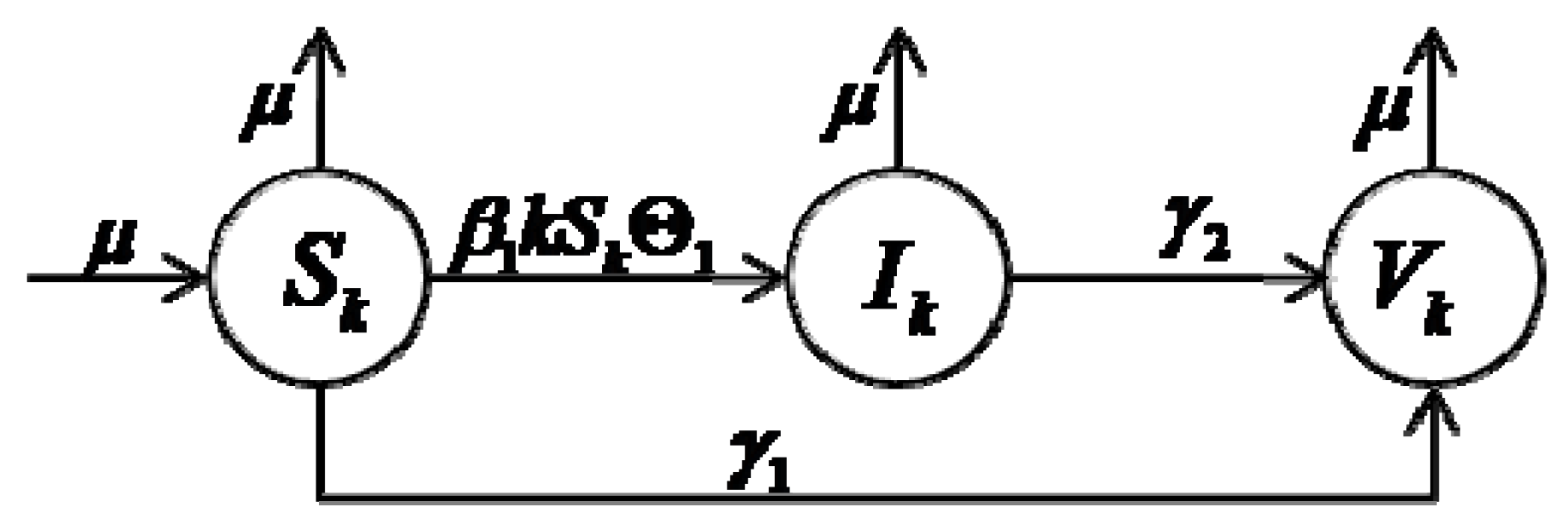
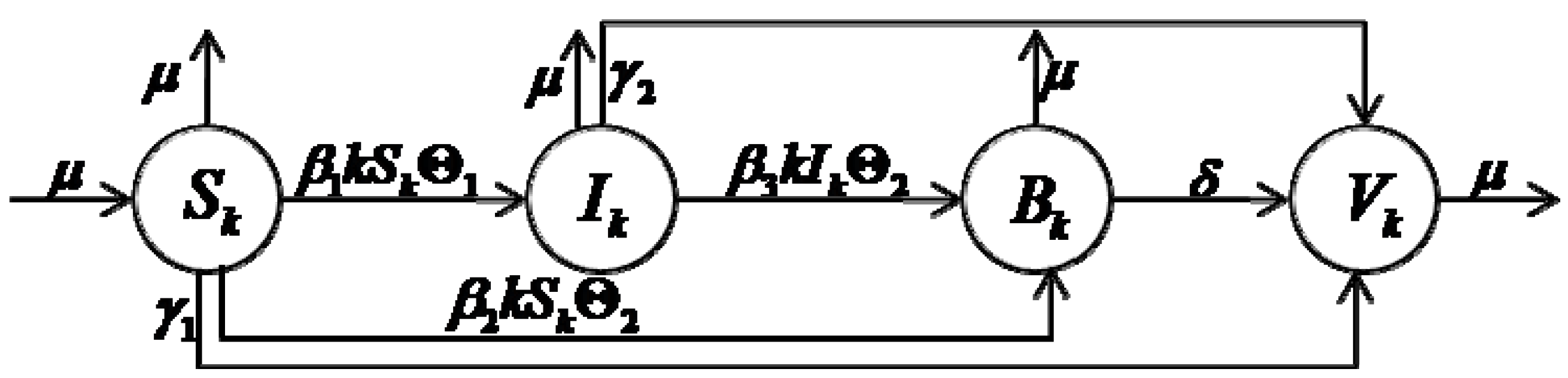
In order to study the influences of the M2M network heterogeneity on worm spreading, in our models, a group $G=(V,E)$ is used to represent the topological structure of the M2M network, where $V$ is the set of all nodes and $E$ is the set of all edges. In this group, a node corresponds to a computer, and an edge represents the potential communication between two nodes. The number of edges emanating from a node is called as the degree of a node. We assume that the total computers can be broken into a number of homogeneous sub-compartments, i.e., all nodes in the same sub-compartment are dynamically equivalent, without any difference. We classify the nodes into compartments based on the number of node degree, i.e., nodes in the same sub-compartment have the same number of node degrees. Our model is based on a system of ordinary differential equations describing the evolution of the number of individuals in each compartment.

Based on the above assumptions, we classify the total nodes into Δ different groups, where $N_k(k=1,2,\mathrm{...},\text{Δ})$ is the total number of nodes that have $k$-degree, and Δ is the maximum node degree of total nodes. $N(N={\displaystyle {\sum }_k{N}_k},k=1,2,\cdots ,\text{Δ})$ is the nodes size of the whole network. In order to reflect the heterogeneous nature of an M2M network, we consider nodes degree distribution $p(k)$, i.e., $p(k)=N_k/N$, which is the probability that a node degree chosen randomly is $k$-degree.

According to our different purposes, the infection rates of nodes can be classified into the following compartments: susceptible nodes $(S)$, malicious infectious nodes $(I)$, benign infectious nodes $(B)$ and recovered nodes $(V)$. The corresponding notations are as following: $S_k(t),I_k(t),B_k(t),V_k(t)$, are, respectively, the relative densities of $S$-nodes, $I$-nodes, $B$-nodes, and $V$-nodes with $k$-degree at time $t$. Some frequently used notations of this paper are listed in Table 1.

Table 1. Notations of this paper.

Δ	The maximum node degree of total nodes
$S_k(t)$	The relative density of -nodes with -degree at time S-nodes with k-degree at time t
$I_k(t)$	The relative density of I-nodes with k-degree at time t
$B_k(t)$	The relative density of B-nodes with k-degree at time t
$V_k(t)$	The relative density of V-nodes with k-degree at time t
$N_k$	The total number of nodes with k-degree
$N$	The nodes size of the whole network
${\beta }_1$	The effective infection rate of the malicious worms
${\beta }_2$	The effective infection rate of the benign worms
${\beta }_3$	The effective repair rate of the benign worms wipe off the malicious worms
${\gamma }_1$	The recovery rate of S-nodes become V-nodes due to the treatment effect
${\gamma }_2$	The recovery rate of I-nodes become V-nodes due to the treatment effect
$\delta$	The self-destruction rate of the benign worms in the B-nodes
$\mu$	The birth or death rate of a node
${\text{Θ}}_1(t)$	The probability that a randomly chosen link points to a I-node
${\text{Θ}}_2(t)$	The probability that a randomly chosen link points to a B-node
$p(k)$	The probability that a node chosen randomly with k-degree

Table 1. Notations of this paper.

Δ	The maximum node degree of total nodes
$S_k(t)$	The relative density of -nodes with -degree at time S-nodes with k-degree at time t
$I_k(t)$	The relative density of I-nodes with k-degree at time t
$B_k(t)$	The relative density of B-nodes with k-degree at time t
$V_k(t)$	The relative density of V-nodes with k-degree at time t
$N_k$	The total number of nodes with k-degree
$N$	The nodes size of the whole network
${\beta }_1$	The effective infection rate of the malicious worms
${\beta }_2$	The effective infection rate of the benign worms
${\beta }_3$	The effective repair rate of the benign worms wipe off the malicious worms
${\gamma }_1$	The recovery rate of S-nodes become V-nodes due to the treatment effect
${\gamma }_2$	The recovery rate of I-nodes become V-nodes due to the treatment effect
$\delta$	The self-destruction rate of the benign worms in the B-nodes
$\mu$	The birth or death rate of a node
${\text{Θ}}_1(t)$	The probability that a randomly chosen link points to a I-node
${\text{Θ}}_2(t)$	The probability that a randomly chosen link points to a B-node
$p(k)$	The probability that a node chosen randomly with k-degree

3.1. The Model of $S_k{I}_k{V}_k$

The $S_k{I}_k{V}_k$ model only contains three compartments: $S$-nodes, $I$-nodes, and $V$-nodes. Figure 1 is the transfer diagram of each compartment with $k$-degree $(k=1,2,\mathrm{...},\text{Δ})$.

Figure 1. The transfer diagram of $S_k{I}_k{V}_k$ model.

Figure 1. The transfer diagram of $S_k{I}_k{V}_k$ model.

In Figure 1, ${\text{Θ}}_1(t)={\displaystyle {\sum }_{k}kp(k)I_k}/{\displaystyle {\sum }_{k}kp(k)}={\displaystyle {\sum }_{k}kp(k)I_k}/<k>=<k_I>/<k>$ represents the probability that a randomly chosen link points to a malicious infectious node, i.e. the relative density of $I$-nodes at time $t$. $\mu$ is the birth or death rate of a node; thus, $S_k(t)+I_k(t)+V_k(t)=1$ is invariable. Due to the infection of the malicious nodes, $S$-nodes becomes $I$-nodes at constant rate ${\beta }_1$. Thus, ${\beta }_{1}k{S}_k{\text{Θ}}_1$ is the number of $S$-nodes turn into $I$-nodes at time $t$. ${\gamma }_1$ and ${\gamma }_2$ are, respectively, the recovery rate of $S$-nodes and $I$-nodes due to the treatment effect of users. Based on Figure 1, we can get the dynamical differential equations for each compartment with $k$-degree as following:

$$\{\begin{array}{l}\frac{d{S}_k(t)}{dt}=\mu -{\beta }_{1}k{S}_k(t){\text{Θ}}_1(t)-({\gamma }_1+\mu )S_k(t)\\ \frac{d{I}_k(t)}{dt}={\beta }_{1}k{S}_k(t){\text{Θ}}_1(t)-({\gamma }_2+\mu )I_k(t)\\ \frac{d{V}_k(t)}{dt}={\gamma }_1{S}_k(t)+{\gamma }_2{I}_k(t)-\mu V_k(t)\end{array}$$

(1)

The initial condition of System (1) is $S_k(0),I_k(0),V_k(0)\ge 0$, and its feasible region is $U_1=\left\{\left(S_k,I_k,V_k\right)\in R_{+}^{3\text{Δ}}:S_k+I_k+V_k\le 1,1\le k\le \text{Δ}\right\}$, which is a positively invariant.

3.2. The Model of $S_k{I}_k{B}_k{V}_k$

In the $S_k{I}_k{B}_k{V}_k$ model, we divide nodes into four compartments: $S$-nodes, $I$-nodes, $B$-nodes and $V$-nodes. The transfer diagram of each compartment with $k$-degree $(k=1,2,\mathrm{...},\text{Δ})$ is schematically depicted in Figure 2.

Figure 2. The transfer diagram of $S_k{I}_k{B}_k{V}_k$ model.

Figure 2. The transfer diagram of $S_k{I}_k{B}_k{V}_k$ model.

In Figure 2, ${\text{Θ}}_2(t)={\displaystyle {\sum }_{k}kp(k)B_k}/{\displaystyle {\sum }_{k}kp(k)}={\displaystyle {\sum }_{k}kp(k)B_k}/<k>=<k_B>/<k>$ represents the probability that a randomly chosen link points to a benign infectious node, i.e., the relative density of $B$-nodes at time $t$. Due to the repair infection of benign nodes, $S$-nodes become $B$-nodes at constant rate ${\beta }_2$ and $I$-nodes become $B$-nodes at constant rate ${\beta }_3$, where ${\beta }_3\le {\beta }_2$. $\delta$ is the self-destruction rate of the benign worms in the $B$-nodes, i.e., the rate $B$-nodes translate into $V$-nodes. Besides, the other model parameters are the same as defined in Figure 1. Based on Figure 2, the dynamical differential equations for each compartment with $k$-degree is donated as:

$$\{\begin{array}{l}\frac{d{S}_k(t)}{dt}=\mu -{\beta }_{1}k{S}_k(t){\text{Θ}}_1(t)-{\beta }_{2}k{S}_k(t){\text{Θ}}_2(t)-({\gamma }_1+\mu )S_k(t)\\ \frac{d{I}_k(t)}{dt}={\beta }_{1}k{S}_k(t){\text{Θ}}_1(t)-{\beta }_{3}k{I}_k(t){\text{Θ}}_2(t)-({\gamma }_2+\mu )I_k(t)\\ \frac{d{B}_k(t)}{dt}={\beta }_{2}k{S}_k(t){\text{Θ}}_2(t)+{\beta }_{3}k{I}_k(t){\text{Θ}}_2(t)-(\delta +\mu )B_k(t)\\ \frac{d{V}_k(t)}{dt}={\gamma }_1{S}_k(t)+{\gamma }_2{I}_k(t)+\delta B_k(t)-\mu V_k(t)\end{array}$$

(2)

The initial condition of System (2) is $S_k(0),I_k(0),V_k(0),B_k(0)\ge 0$, and its feasible region is $U_2=\left\{\left(S_k,I_k,V_k,B_k\right)\in R_{+}^{4\text{Δ}}:S_k+I_k+V_k+B_k\le 1,1\le k\le \text{Δ}\right\}$, which is a positively invariant.

3.3. The $S_k{I}_k{V}_k$ Model Based on Targeted Immunization Strategy

The endemic equilibrium of System (1) is $I_k^{*}=\frac{{\beta }_{1}k{S}_k^{*}{\text{Θ}}_1}{{\gamma }_2+\mu }=\frac{\mu {\beta }_{1}k{\text{Θ}}_1}{({\gamma }_2+\mu )({\beta }_{1}k{\text{Θ}}_1+{\gamma }_1+\mu )}$. It is easy to know $I_1^{*}<I_2^{*}<\cdots <I_{\text{Δ}}^{*}$ and $\underset{k\to \infty }{\lim }{I}_k^{*}=\frac{\mu }{{\gamma }_2+\mu }$. This indicates that a node with a higher node degree is more susceptible to be infected by worms than that with a lower node degree. In addition, we can conclude that the higher the degree of nodes, the higher the infection density of a network, and thus the density would tend to a constant when the node degree goes to infinity. Indeed, this precisely coincides with reality. Thus, we can use targeted immunization strategy to strengthen protection efforts of the nodes that have a higher node degree [37]. First, we introduce lower and upper thresholds $K_1$ and $K_2$, such that if $k>K_2$, all nodes with $k$-degree will be immunized, while if $K_1\le k\le K_2$, a fraction $a(0<a<1)$ of nodes with $k$-degree will be immunized. Thus, we can define the immunization rate ${\eta }_k$ as following:

$${\eta }_k=\{\begin{array}{l}1(k>K_2)\\ a(K_1\le k\le K_2)\\ 0(k<K_1)\end{array}$$

Thus, $\overline{\eta }={\displaystyle {\sum }_k{\eta }_{k}p(k)}$ is the average immunization rate of the targeted immunization strategy. Then, the ordinary differential equations of System (1) will become

$$\{\begin{array}{l}\frac{d{S}_k(t)}{dt}=\mu -{\beta }_{1}k(1-{\eta }_k)S_k(t){\text{Θ}}_1-({\gamma }_1+\mu )S_k(t)\\ \frac{d{I}_k(t)}{dt}={\beta }_{1}k(1-{\eta }_k)S_k(t){\text{Θ}}_1-({\gamma }_2+\mu )I_k(t)\\ \frac{d{V}_k(t)}{dt}={\gamma }_1{S}_k(t)+{\gamma }_2{I}_k(t)-\mu V_k(t)\end{array}$$

(3)

The feasible region of System (3) is same with System (1).

4. The Global Stability of Models

4.1. The Global Stability of $S_k{I}_k{V}_k$ Model

By counting, we can easily obtain the equilibrium of System (1). The worm-free equilibrium is $E_0=(\frac{\mu }{{\gamma }_1+\mu },0,\frac{{\gamma }_1}{{\gamma }_1+\mu },\cdots ,\frac{\mu }{{\gamma }_1+\mu },0,\frac{{\gamma }_1}{{\gamma }_1+\mu })$, i.e., $S_k^0=\frac{\mu }{{\gamma }_1+\mu },I_k^0=0,V_k^0=\frac{{\gamma }_1}{{\gamma }_1+\mu },k=1,2,\cdots \text{Δ}$; and the endemic equilibrium is $E^{*}=(S_1^{*},I_1^{*},V_1^{*},\cdots ,S_{\text{Δ}}^{*},I_{\text{Δ}}^{*},V_{\text{Δ}}^{*})$, where $S_k^{*}=\frac{\mu }{{\beta }_{1}k{\text{Θ}}_1+{\gamma }_1+\mu },I_k^{*}=\frac{{\beta }_{1}k{S}_k^{*}{\text{Θ}}_1}{{\gamma }_2+\mu },$ $V_k^{*}=1-S_k^{*}-I_k^{*},k=1,2,\cdots ,\text{Δ}$, meanwhile, $S_k^{*},I_k^{*},V_k^{*}>0$. According to the computing method in [38], only the infected compartment $I_k$ is involved in the calculation of the basic reproductive number $R_0$. At the worm-free equilibrium $E_0$, the transmission matrix $F$ is the rate of appearance of new infections and the transmission matrix $W$is the transfer rate of nodes among compartments; they are, respectively, denoted by

$$F=\left(\begin{array}{cc}A& 0_{\text{Δ}\times \text{Δ}}\\ 0_{\text{Δ}\times \text{Δ}}& 0_{\text{Δ}\times \text{Δ}}\end{array}\right),W=\left(\begin{array}{cc}Q& 0_{\text{Δ}\times \text{Δ}}\\ 0_{\text{Δ}\times \text{Δ}}& 0_{\text{Δ}\times \text{Δ}}\end{array}\right),$$

where

$$A=\frac{{\beta }_1}{<k>}\left[\begin{array}{l}1\\ 2\\ ⋮\\ \text{Δ}\end{array}\right]\left[1p(1),2p(2),\cdots ,\text{Δ}p(\text{Δ})\right],Q=({\gamma }_2+\mu )E_{\text{Δ}}$$

($E_{\text{Δ}}$ is the $\text{Δ}\times \text{Δ}$ identity matrix). Hence, $W^{-1}=\left(\begin{array}{cc}{Q}^{-1}& 0_{\text{Δ}\times \text{Δ}}\\ 0_{\text{Δ}\times \text{Δ}}& 0_{\text{Δ}\times \text{Δ}}\end{array}\right)$. Therefore, according to Theorems in [38,39], the basic reproduction number R₀ is defined as the spectral radius of the next generation matrix $F{W}^{-1}$; that is,

$$R_{01}=\rho (F{W}^{-1})=\rho (A{Q}^{-1})=\frac{{\beta }_1}{{\gamma }_2+\mu }\cdot \frac{<k^2>}{<k>}$$

Based on $R_{01}$, we have the following theorem:

Theorem 1. When $R_{01}\le 1$, the worm-free equilibrium $E^{*}$ of System (1) is locally and globally asymptotically stable in the model’s feasible region $U_1$, and unstable when $R_{01}>1$.

Proof. To measure the global asymptotical stability of worm-free equilibrium, we choose a Lyapunov function like this: $L_1(t)={\displaystyle {\sum }_k\frac{k}{{\gamma }_2+\mu }p(k)I_k(t)}$. Hence, the time derivative of $L_1(t)$ along the solutions of System (1) is formulated as following:

$$\begin{array}{l}{L_1}^{\text{'}}(t)={\displaystyle {\sum }_k\frac{k}{{\gamma }_2+\mu }p(k)\left[{\beta }_{1}k{S}_k{\text{Θ}}_1-({\gamma }_2+\mu )I_k\right]}\\ ={\displaystyle {\sum }_k\frac{{\beta }_1{S}_k{\text{Θ}}_1}{{\gamma }_2+\mu }{k}^{2}p(k)-{\displaystyle {\sum }_{k}kp(k)I_k}}\\ \le {\displaystyle {\sum }_k\frac{{\beta }_1{\text{Θ}}_1}{{\gamma }_2+\mu }{k}^{2}p(k)-{\displaystyle {\sum }_{k}kp(k)I_k}}\\ =\frac{{\beta }_1{\text{Θ}}_1<k^2>}{{\gamma }_2+\mu }-{\text{Θ}}_1<k>\\ ={\text{Θ}}_1<k>\left(\frac{{\beta }_1}{{\gamma }_2+\mu }\cdot \frac{<k^2>}{<k>}-1\right)\\ ={\text{Θ}}_1<k>\left(R_{01}-1\right)\end{array}$$

We can know that ${L_1}^{\text{'}}(t)=0$ only if $R_{01}=1$. Therefore, according to LaSalle’s invariance principle [40], when $R_{01}\le 1$, the worm-free equilibrium $E_0$ of System (1) is locally and globally asymptotically stable in the model’s feasible region $U_1$. When $R_{01}>1$, it means that $L_1{(t)}^{\text{'}}>0$, and $E_0$ is unstable in $U_1$. Thus, Theorem 1 is proved. □

4.2. The Global Stability of $S_k{I}_k{B}_k{V}_k$ Model

The worm-free equilibrium of System (2) is $E_0=(\frac{\mu }{{\gamma }_1+\mu },0,0,\frac{{\gamma }_1}{{\gamma }_1+\mu },\cdots ,\frac{\mu }{{\gamma }_1+\mu },0,0,\frac{{\gamma }_1}{{\gamma }_1+\mu })$, which means $S_k^0=\frac{\mu }{{\gamma }_1+\mu },I_k^0=0,B_k^0=0,V_k^0=\frac{{\gamma }_1}{{\gamma }_1+\mu },k=1,2,\cdots ,\text{Δ};$ and the endemic equilibrium is $E^{*}=(S_1^{*},I_1^{*},B_1^{*},V_1^{*},\cdots ,S_{\text{Δ}}^{*},I_{\text{Δ}}^{*},B_{\text{Δ}}^{*},V_{\text{Δ}}^{*})$, where

$$\begin{array}{l}{S}_k^{*}=\frac{\mu }{{\beta }_{1}k{\text{Θ}}_1+{\beta }_{2}k{\text{Θ}}_2+{\gamma }_1+\mu },I_k^{*}=\frac{{\beta }_{1}k{S}_k^{*}{\text{Θ}}_1}{{\beta }_{3}k{\text{Θ}}_2+{\gamma }_2+\mu },\\ B_k^{*}=\frac{{\beta }_{2}k{S}_k^{*}{\text{Θ}}_2+{\beta }_{3}k{I}_k^{*}{\text{Θ}}_2}{\delta +\mu },V_k^{*}=1-S_k^{*}-I_k^{*}-B_k^{*},k=1,2,\cdots ,\text{Δ}.\end{array}$$

Meanwhile, $S_k^{*},I_k^{*},B_k^{*},V_k^{*}>0$. Similarly, let $F_1=\left(\begin{array}{cc}{A}_1& 0_{\text{Δ}\times \text{Δ}}\\ 0_{\text{Δ}\times \text{Δ}}& 0_{\text{Δ}\times \text{Δ}}\end{array}\right),W_1=\left(\begin{array}{cc}{Q}_1+C& 0_{\text{Δ}\times \text{Δ}}\\ 0_{\text{Δ}\times \text{Δ}}& 0_{\text{Δ}\times \text{Δ}}\end{array}\right)$, where

$$A_1=\frac{{\beta }_1}{<k>}\left[\begin{array}{l}1\\ 2\\ ⋮\\ \text{Δ}\end{array}\right]\left[1p(1),2p(2),\cdots ,\text{Δ}p(\text{Δ})\right],Q_1=\frac{{\beta }_3}{<k>}\left[\begin{array}{l}1\\ 2\\ ⋮\\ \text{Δ}\end{array}\right]\left[1p(1),2p(2),\cdots ,\text{Δ}p(\text{Δ})\right]$$

$C=({\gamma }_2+\mu )E_{\text{Δ}}$ ($E_{\text{Δ}}$ is the $\text{Δ}\times \text{Δ}$ identity matrix). Hence, ${W_1}^{-1}=\left(\begin{array}{cc}{(Q_1+C)}^{-1}& 0_{\text{Δ}\times \text{Δ}}\\ 0_{\text{Δ}\times \text{Δ}}& 0_{\text{Δ}\times \text{Δ}}\end{array}\right)$. According to Theorems in [38,39], the basic reproduction number R₀ is defined as the spectral radius of the next generation matrix $F_1{W_1}^{-1}$, the reproductive number is

$$R_{02}=\rho (F_1{W_1}^{-1})=\rho (A_1{(Q_1+C)}^{-1})=\frac{{\beta }_1<k^2>}{{\beta }_3<k^2>+({\gamma }_2+\mu )<k>}.$$

Based on $R_{02}$, we have the following theorems:

Theorem 2. When $R_{02}\le 1$, the worm-free equilibrium $E^{*}$ of System (2) is locally and globally asymptotically stable in the model’s feasible region $U_2$, and unstable when $R_{02}>1$.

Proof. To measure the global asymptotical stability of worm-free equilibrium, we choose a Lyapunov function like this: $L_2(t)={\displaystyle {\sum }_{k}kp(k)I_k(t)}$. Hence, the time derivative of $L_2(t)$ along the solutions of System (2) is formulated as:

$$\begin{array}{l}{L_2}^{\text{'}}(t)={\displaystyle {\sum }_{k}kp(k)\left[{\beta }_{1}k{S}_k{\text{Θ}}_1-{\beta }_{3}k{I}_k{\text{Θ}}_2-({\gamma }_2+\mu )I_k\right]}\\ ={\displaystyle {\sum }_k{\beta }_1{S}_k{\text{Θ}}_1{k}^{2}p(k)-{\displaystyle {\sum }_k{\beta }_3{I}_k{\text{Θ}}_2{k}^{2}p(k)}-({\gamma }_2+\mu ){\displaystyle {\sum }_{k}kp(k)I_k}}\\ \le {\displaystyle {\sum }_k{\beta }_1{\text{Θ}}_1{k}^{2}p(k)-{\displaystyle {\sum }_k{\beta }_3{I}_k{\text{Θ}}_2{k}^{2}p(k)}-({\gamma }_2+\mu ){\displaystyle {\sum }_{k}kp(k)I_k}}\\ ={\beta }_1{\text{Θ}}_1<k^2>-{\displaystyle {\sum }_k{\beta }_3{I}_k{\text{Θ}}_2{k}^{2}p(k)}-({\gamma }_2+\mu ){\text{Θ}}_1<k>\\ =\left({\displaystyle {\sum }_k{\beta }_3{I}_k{\text{Θ}}_2{k}^{2}p(k)}+({\gamma }_2+\mu ){\text{Θ}}_1<k>\right)\left(\frac{{\beta }_1{\text{Θ}}_1<k^2>}{{\displaystyle {\sum }_k{\beta }_3{I}_k{\text{Θ}}_2{k}^{2}p(k)+({\gamma }_2+\mu ){\text{Θ}}_1<k>}}-1\right)\\ =\left({\displaystyle {\sum }_k{\beta }_3{I}_k{\text{Θ}}_2{k}^{2}p(k)}+({\gamma }_2+\mu ){\text{Θ}}_1<k>\right)\left(\frac{{\beta }_1<k^2>}{{\displaystyle {\sum }_k{\beta }_3(I_k{\text{Θ}}_2{{\text{Θ}}_1}^{-1})k^{2}p(k)+({\gamma }_2+\mu )<k>}}-1\right)\\ =\left({\displaystyle {\sum }_k{\beta }_3{I}_k{\text{Θ}}_2{k}^{2}p(k)}+({\gamma }_2+\mu ){\text{Θ}}_1<k>\right)\left(\frac{{\beta }_1<k^2>}{{\displaystyle {\sum }_k{\beta }_3(I_k\frac{{\displaystyle {\sum }_{k}kp(k)B_k}}{{\displaystyle {\sum }_{k}kp(k)I_k}})k^{2}p(k)+({\gamma }_2+\mu )<k>}}-1\right)\end{array}$$

At $E_0$, $I_k^0=0$ and $B_k^0=0$, thus

$$\begin{array}{l}{L_2}^{\text{'}}(t)\le \left({\displaystyle {\sum }_k{\beta }_3{I}_k{\text{Θ}}_2{k}^{2}p(k)}+({\gamma }_2+\mu ){\text{Θ}}_1<k>\right)\left(\frac{{\beta }_1<k^2>}{{\beta }_3<k^2>+({\gamma }_2+\mu )<k>}-1\right)\\ =\left({\displaystyle {\sum }_k{\beta }_3{I}_k{\text{Θ}}_2{k}^{2}p(k)}+({\gamma }_2+\mu ){\text{Θ}}_1<k>\right)\left(R_{02}-1\right).\end{array}$$

We can know that ${L_2}^{\text{'}}(t)=0$ only if $R_{02}=1$. Therefore, according to LaSalle’s invariance principle [40], when $R_{02}\le 1$, the worm-free equilibrium $E_0$ of System (2) is locally and globally asymptotically stable in the model’s feasible region $U_2$. Otherwise, $E_0$ is unstable in $U_2$. Thus, Theorem 2 is proved. □

4.3. The Basic Reproductive Number of System (3)

We have known that the initial condition, and the worm-free equilibrium of System (3) are the same as System (1). Besides, the endemic equilibrium of System (3) is $E^{*}=(S_1^{*},I_1^{*},V_1^{*},\cdots ,S_{\text{Δ}}^{*},I_{\text{Δ}}^{*},V_{\text{Δ}}^{*})$, where $S_k^{*}=\frac{\mu }{{\beta }_{1}k(1-{\eta }_k){\text{Θ}}_1+{\gamma }_1+\mu },I_k^{*}=\frac{{\beta }_{1}k(1-{\eta }_k)S_k^{*}{\text{Θ}}_1}{{\gamma }_2+\mu },V_k^{*}=1-S_k^{*}-I_k^{*},k=1,2,\cdots ,\text{Δ}$, and $S_k^{*},I_k^{*},V_k^{*}>0$. By counting, we can also obtain that the basic reproduction number of System (3) is

$$R_{03}=\frac{{\beta }_1}{({\gamma }_2+\mu )}\cdot \frac{<k^2(1-{\eta }_k)>}{<k>}=\frac{{\beta }_1}{({\gamma }_2+\mu )}\cdot \frac{<k^2>-<{\eta }_k{k}^2>}{<k>}.$$

Because $<{\eta }_k{k}^2>=\overline{\eta }<k^2>+\phi$, where $\phi$ is the covariance of ${\eta }_k$ and $k^2$, and $\phi =Cov({\eta }_k,k^2)=<({\eta }_k-\overline{\eta })(k^2-<k^2>)>$. Thus, when choosing an appropriately small value of $K_2$, we can ensure $\phi >0$, here,

$$R_{03}=\frac{{\beta }_1}{({\gamma }_2+\mu )}\cdot \frac{<k^2>(1-\overline{\eta })-\phi }{<k>}<\frac{{\beta }_1}{({\gamma }_2+\mu )}\cdot \frac{<k^2>(1-\overline{\eta })}{<k>}=R_{01}(1-\overline{\eta }).$$

5. The Final Size Formula if $R_0>1$

The expected final size of worms is defined as the total number of nodes affected by the worm at the end of the epidemic, which is an important indicator of worm outbreak. In this section, by using the same computing method in [38], we will firstly investigate the final size formula of System (2). Secondly, we will get the final size formula of worms based on the comprehensive immunization scheme.

5.1. The Final Size Formula of System (2)

First, we show that the worms of System (2) will eventually die out, i.e., $I_k(+\infty )=0,B_k(\infty )=0,1\le k\le \text{Δ}.$ Since the positively invariance of System (2) is $0\le S_k,I_k,B_k,V_k\le 1,S_k+I_k+B_k+V_k=1,1\le k\le \text{Δ}$, we know that all solutions of System (2) are non-negative and bounded.

In the absence of birth, death and the treatment effect of users, $\mu ={\gamma }_1={\gamma }_2=0$. Then

$$\frac{d}{dt}(S_k(t)+I_k(t))=-{\beta }_{2}k{S}_k(t){\text{Θ}}_2-{\beta }_{3}k{I}_k(t){\text{Θ}}_2$$

(4)

We see that $S_k(t)+I_k(t)$ is strictly decreasing whenever $I_k(t)>0$. Because $S_k(t)+I_k(t)$ is bounded below by zero, it has a limit as $t\to \infty$. Because $S_k(t)$ is decreasing and also bounded by zero, it also has a limit as $t\to \infty$. Therefore, $I_k(t)$ will tend to zero; that is, $I_k(\infty )=0$. Due to

$$\frac{d}{dt}(S_k(t)+I_k(t)+B_k(t))=-\delta B_k(t)$$

(5)

Evidenced by the same token, we know that $B_k(t)$ tends to zero; that is, $B_k(\infty )=0$. We adopt the convention that, for any non-negative continuous function $f(t)$, $f_{\infty }=\underset{t\to \infty }{\lim }f(t)$, and $\overline{f}={\displaystyle {\int }_0^{\infty }f(t)dt}$, since

$$\frac{d{S}_k(t)}{dt}=-{\beta }_{1}k{S}_k(t){\text{Θ}}_1-{\beta }_{2}k{S}_k(t){\text{Θ}}_2$$

(6)

If we integrate Equation (6) from 0 to ∞, we can obtain

$$S_k(t)-S_k(0)=-{\displaystyle {\int }_0^t\left({\beta }_{1}k{S}_k(\tau ){\text{Θ}}_1(\tau )+{\beta }_{2}k{S}_k(\tau ){\text{Θ}}_2(\tau )\right)d\tau }$$

(7)

Due to

$${\displaystyle {\int }_0^t{\text{Θ}}_1(\tau )d\tau }=\frac{{\displaystyle {\sum }_{k}kp(k){\displaystyle {\int }_0^t{I}_k(\tau )d\tau }}}{<k>}$$

$${\displaystyle {\int }_0^t{\text{Θ}}_2(\tau )d\tau }=\frac{{\displaystyle {\sum }_{k}kp(k){\displaystyle {\int }_0^t{B}_k(\tau )d\tau }}}{<k>}$$

(8)

When $t\to \infty$, we get ${\overline{\text{Θ}}}_1=\frac{{\displaystyle {\sum }_{k}kp(k){\overline{I}}_k}}{<k>}$ and ${\overline{\text{Θ}}}_2=\frac{{\displaystyle {\sum }_{k}kp(k){\overline{B}}_k}}{<k>}$.

From Equation (7), we get

$${\overline{S}}_k=\frac{S_k(0)-S_k(\infty )}{{\beta }_{1}k{\overline{I}}_k+{\beta }_{2}k{\overline{B}}_k}, \mathrm{as} t\to \infty$$

(9)

Through similar calculation, we obtain

$${\overline{I}}_k=\frac{I_k(0)}{{\beta }_{3}k{\overline{B}}_k-{\beta }_{1}k{\overline{S}}_k} \mathrm{and} {\overline{B}}_k=\frac{B_k(0)}{\delta -{\beta }_{2}k{\overline{S}}_k-{\beta }_{3}k{\overline{I}}_k}$$

(10)

From Equations (9) and (10), we can calculate that

$${\overline{B}}_k=\frac{S_k(0)-S_k(\infty )+I_k(0)+B_k(0)}{\delta } \mathrm{and} {\overline{I}}_k=\frac{M+\sqrt{M^2+{\beta }_1{{\beta }_2}^2{k}^3{I}_k(0)}}{2{\beta }_1{\beta }_2{k}^2}$$

(11)

where

$$M=\frac{{\beta }_{1}k{\delta }^2[S_k(0)-S_k(\infty )+I_k(0)]-{{\beta }_2}^2{k}^2{[S_k(0)-S_k(\infty )+I_k(0)+B_k(0)]}^2}{\delta [S_k(0)-S_k(\infty )+I_k(0)+B_k(0)]}$$

(12)

Integrating System (2) from 0 to $t$, we get

$$\begin{array}{l}\ln \frac{S_k(0)}{S_k(t)}={\displaystyle {\int }_0^t\left({\beta }_{1}k{\text{Θ}}_1(\tau )+{\beta }_{2}k{\text{Θ}}_2(\tau )\right)d\tau }\\ =\frac{{\beta }_{1}k}{<k>}{\displaystyle \sum _{k}kp(k){\displaystyle {\int }_0^t{I}_k(\tau )d\tau }}+\frac{{\beta }_{2}k}{<k>}{\displaystyle \sum _{k}kp(k){\displaystyle {\int }_0^t{B}_k(\tau )d\tau }}\end{array}$$

Letting $t\to \infty$, we have

$$\begin{array}{l}\ln \frac{S_k(0)}{S_k(\infty )}={\displaystyle {\int }_0^{\infty }\left({\beta }_{1}k{\text{Θ}}_1(\tau )+{\beta }_{2}k{\text{Θ}}_2(\tau )\right)d\tau }\\ =\frac{{\beta }_{1}k}{<k>}{\displaystyle {\sum }_{k}kp(k)\frac{M+\sqrt{M^2+{\beta }_1{{\beta }_2}^2{k}^3{I}_k(0)}}{2{\beta }_1{\beta }_2{k}^2}}+\frac{{\beta }_{2}k}{<k>}{\displaystyle {\sum }_{k}kp(k)\frac{S_k(0)-S_k(\infty )+I_k(0)+B_k(0)}{\delta }}\end{array}$$

(13)

Consider three cases:

Case 1: If $S_k(0)=S_{k0},I_k(0)=0,B_k(0)=0$, then we have

$$\ln \frac{S_{k0}}{S_{k\infty }}=\frac{k}{<k>\delta {\beta }_2}{\displaystyle {\sum }_{k}kp(k)[{\beta }_1{\delta }^2-{{\beta }_2}^{2}k(S_{k0}-S_{k\infty })]}+\frac{{\beta }_{2}k}{<k>\delta }{\displaystyle {\sum }_{k}kp(k)(S_{k0}-S_{k\infty })}$$

Case 2: If $S_k(0)=S_{k0},I_k(0)=I_{k0},B_k(0)=0$, then we have

$$\ln \frac{S_{k0}}{S_{k\infty }}=k{\displaystyle {\sum }_k\frac{p(k)\left\{\left[{\beta }_1{\delta }^2-{{\beta }_2}^{2}kG\right]+\sqrt{{[{\beta }_1{\delta }^2-{{\beta }_2}^{2}kG]}^2+{\delta }^2{\beta }_1{{\beta }_2}^{2}k{I}_{k0}}\right\}}{2<k>\delta {\beta }_2}}+\frac{{\beta }_{2}k}{<k>\delta }{\displaystyle {\sum }_{k}kp(k)G}$$

$$G=S_{k0}-S_{k\infty }+I_{k0}$$

Case 3: If $S_k(0)=S_{k0},I_k(0)=I_{k0},B_k(0)=B_{k0}$, then we have

$$\ln \frac{S_{k0}}{S_{k\infty }}=k{\displaystyle {\sum }_k\frac{p(k)\left\{\left[{\beta }_1{\delta }^{2}G-{{\beta }_2}^{2}k{J}^2\right]+\sqrt{{[{\beta }_1{\delta }^{2}G-{{\beta }_2}^{2}k{J}^2]}^2+{\delta }^2{J}^2{\beta }_1{{\beta }_2}^{2}k{I}_{k0}}\right\}}{2\delta {\beta }_{2}J<k>}}+\frac{{\beta }_{2}k}{<k>\delta }{\displaystyle {\sum }_{k}kp(k)J}$$

$$J=S_{k0}-S_{k\infty }+I_{k0}+B_{k0}$$

We know the final size formula is $V(\infty )={\displaystyle {\sum }_{k}p(k)V_{k\infty }}=1-{\displaystyle {\sum }_{k}p(k)S_{k\infty }}$, which is related to the network structure. When other parameters do not change, the degree distribution of the network greatly affects the final size of worms; meanwhile, the higher initial value or more effective infection ability of malicious worms, the larger-scale of malicious worms will be.

5.2. The Final Size Formula Based on Comprehensive Immunization Scheme

Since the compiler program of benign worm needs time, we should use the targeted immunization scheme to protect the security of a network before benign worms are put into a network. When benign worm has been compiled, we will only use benign worm scheme to repair a network. That is, from 0 to $T$, we will only use targeted immunization scheme, and only use benign worm scheme from $T$ to $t(t>T)$. Then, we have

$$\begin{array}{l}\ln \frac{S_k(0)}{S_k(t)}={\displaystyle {\int }_0^T{\beta }_{1}k(1-{\eta }_k){\text{Θ}}_1(\tau )d\tau }+{\displaystyle {\int }_T^t\left({\beta }_{1}k{\text{Θ}}_1(\tau )+{\beta }_{2}k{\text{Θ}}_2(\tau )\right)d\tau }\\ =\frac{-{\eta }_k{\beta }_{1}k}{<k>}{\displaystyle \sum _{k}kp(k){\displaystyle {\int }_0^T{I}_k(\tau )d\tau }}+\frac{{\beta }_{1}k}{<k>}{\displaystyle \sum _{k}kp(k){\displaystyle {\int }_0^t{I}_k(\tau )d\tau }}+\frac{{\beta }_{2}k}{<k>}{\displaystyle \sum _{k}kp(k){\displaystyle {\int }_T^t{B}_k(\tau )d\tau }}\end{array}$$

Letting $t\to \infty$, and $S_k(0)=S_{k0},I_k(0)=I_{k0},B_k(0)=B_{k0}$, we have

$$\begin{array}{l}\ln \frac{S_k(0)}{S_k(\infty )}=\frac{{\beta }_{1}k}{<k>}{\displaystyle \sum _{k}kp(k){\displaystyle {\int }_0^{\infty }{I}_k(\tau )d\tau }}+\frac{{\beta }_{2}k}{<k>}{\displaystyle \sum _{k}kp(k){\displaystyle {\int }_T^{\infty }{B}_k(\tau )d\tau }}-\frac{{\eta }_k{\beta }_{1}k}{<k>}{\displaystyle \sum _{k}kp(k){\displaystyle {\int }_0^T{I}_k(\tau )d\tau }}\\ =k{\displaystyle {\sum }_k\frac{p(k)\left\{\left[{\beta }_1{\delta }^{2}G-{{\beta }_2}^{2}k{J}^2\right]+\sqrt{{[{\beta }_1{\delta }^{2}G-{{\beta }_2}^{2}k{J}^2]}^2+{\delta }^2{J}^2{\beta }_1{{\beta }_2}^{2}k{I}_{k0}}\right\}}{2\delta {\beta }_{2}J<k>}}\\ +\frac{{\beta }_{2}k}{<k>}{\displaystyle {\sum }_{k}kp(k)\left[\frac{J}{\delta }+B_{k0}-B_k(T)\right]}+\frac{{\eta }_k{\beta }_{1}k}{<k>}{\displaystyle \sum _{k}kp(k)\left[I_{k0}-I_k(T)\right]}\end{array}$$

The final size formula is $V(\infty )={\displaystyle {\sum }_{k}p(k)V_{k\infty }}=1-{\displaystyle {\sum }_{k}p(k)S_{k\infty }}$, which is also related to the network structure.

6. Simulations

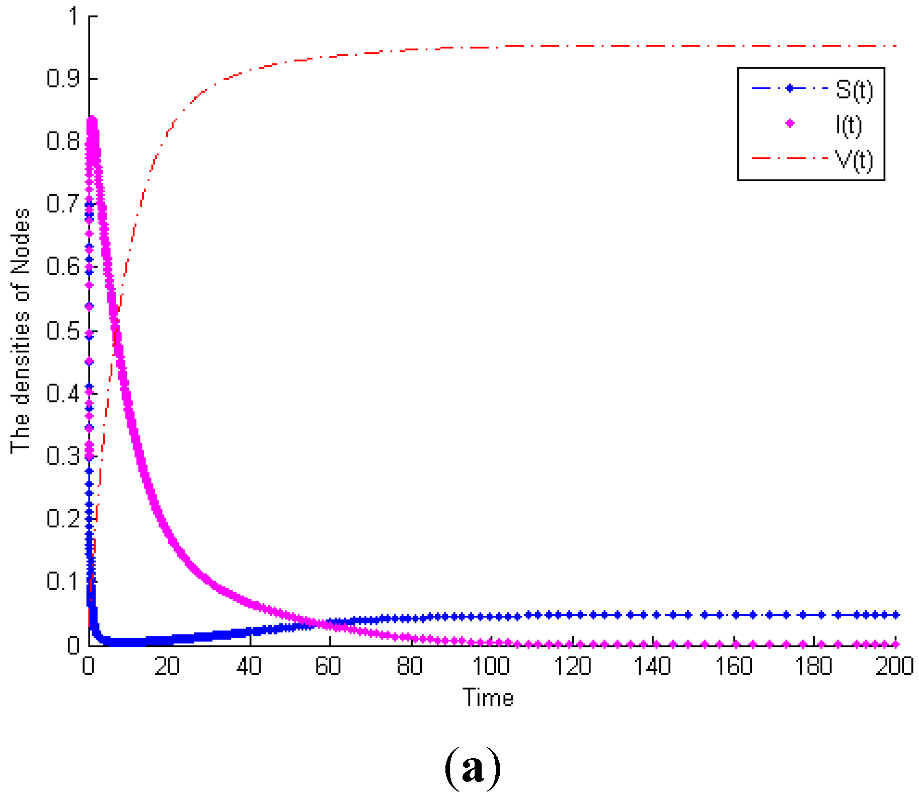
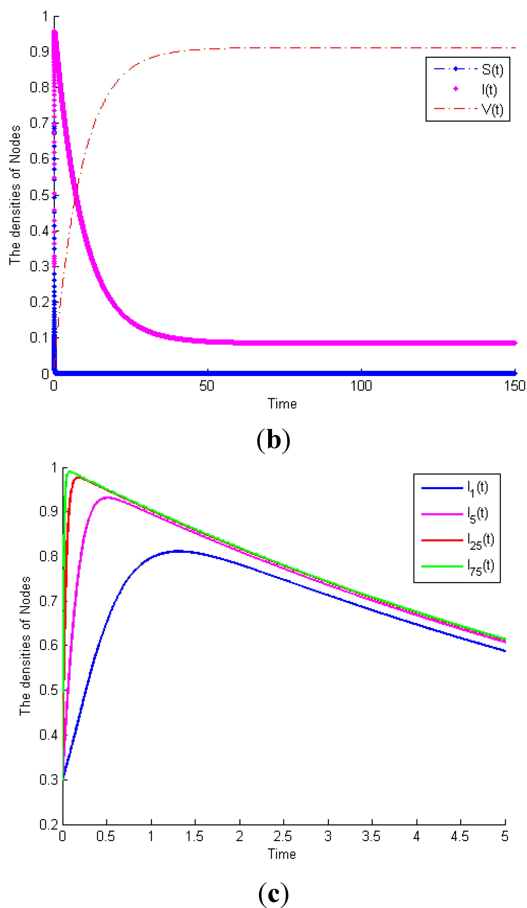
In the real world, the degree distribution of network usually obeys a power-law distribution. We choose $p(k)=2m^2{k}^{-v}(m=3andv=3)$, $\text{Δ}=100$, $N={10}^5$ and $\mu =0.01$, then we get $<k>=29.4297$ and $<k^2>=93.3728$. We use MATLAB simulation tool to verify our theoretical analysis.

Example 1. Consider System (1) with ${\beta }_1=0.01,{\gamma }_1=0.2,{\gamma }_2=0.1,S_k=0.7,I_k=0.3,V_k=0,1\le k\le \text{Δ}$, then $R_{01}=0.2884<1$. Figure 3a exhibits the time plot of System (1). It shows that the malicious worms will gradually disappear. When ${\beta }_1=0.1$ and the other parameters remain the same, $R_{01}=2.8843>1$. Figure 3b shows that the malicious worms are prevalent in the network and all states reach their equilibrium points. This example proves Theorem 1. Furthermore, considering System (1) with the same parameters as Figure 3b, Figure 3c exhibits the time plot of different node degrees of malicious infectious nodes. It shows that a higher node degree host is more susceptible to be infected than a lower node degree host.

Figure 3. (a) Globally asymptotically stable of worm-free equilibrium of System (1) when $R_{01}=0.2884<1$. (b) Malicious worms of System (1) are prevalent when $R_{01}=2.8843>1$. (c) The time plot of different node degrees of malicious infectious nodes.

Figure 3. (a) Globally asymptotically stable of worm-free equilibrium of System (1) when $R_{01}=0.2884<1$. (b) Malicious worms of System (1) are prevalent when $R_{01}=2.8843>1$. (c) The time plot of different node degrees of malicious infectious nodes.

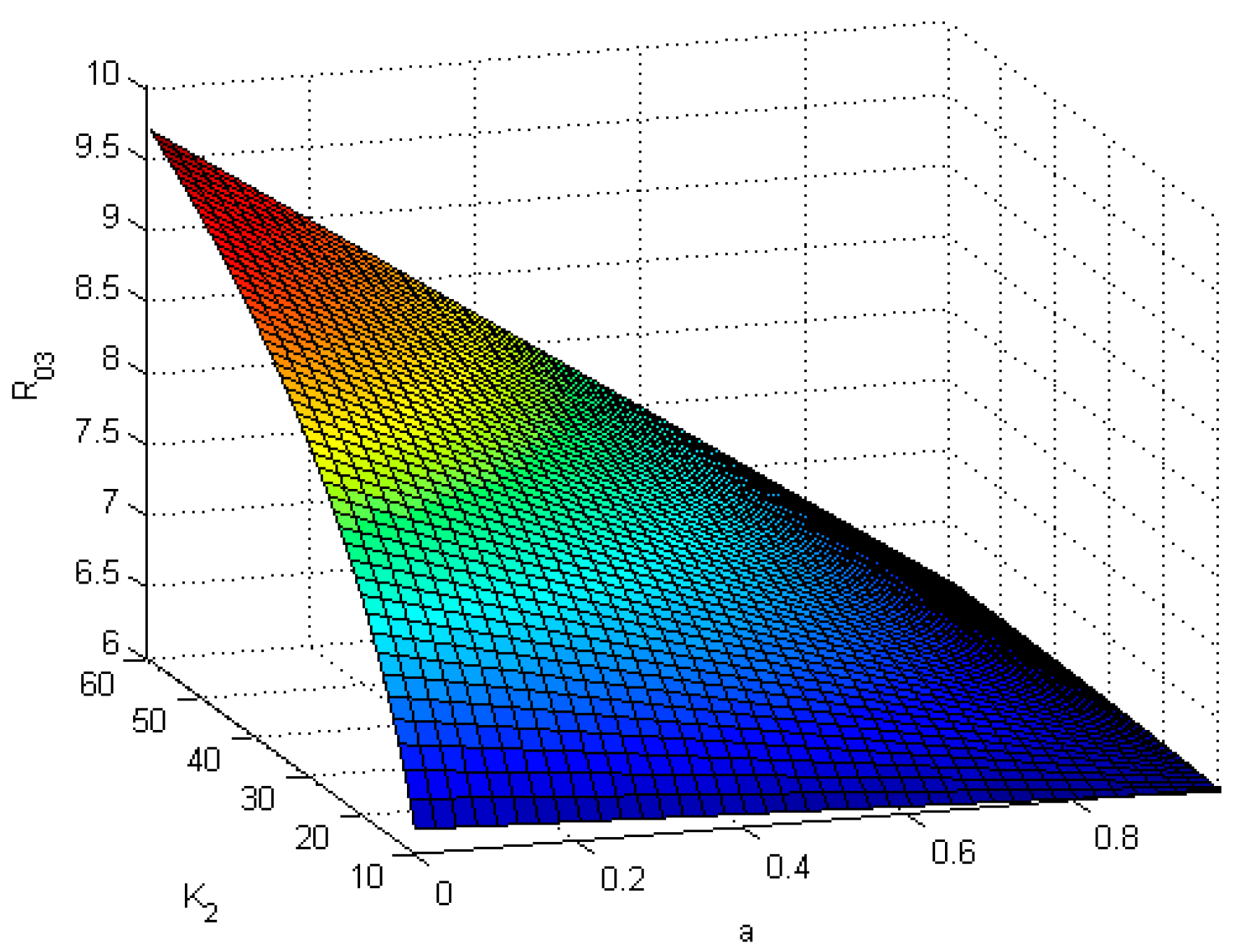
Example 2: Consider System (3) with ${\beta }_1=0.1,{\gamma }_2=0.02,\mu =0.01,K_1=10$, Figure 4 shows that $R_{03}$ is a function of $a$ and $K_2$. It illustrates that $R_{03}$ is a decreasing function of $a$ but an increasing function of $K_2$, which means, if $a$ is large or $K_2$ is small, more nodes will be immune.

Figure 4. $R_{03}$ is a function of $a$ and $K_2$.

Figure 4. $R_{03}$ is a function of $a$ and $K_2$.

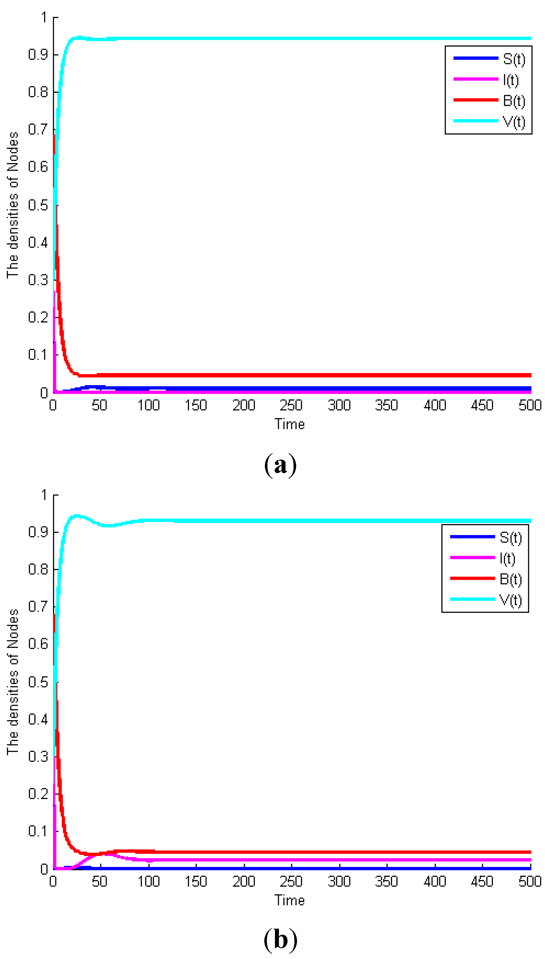
Example 3: Consider System (2) with $\delta =0.2,{\beta }_1=0.01,{\beta }_2=0.04,{\beta }_3=0.02,{\gamma }_1=0.02,{\gamma }_2=0.01,$ $S_k=0.6,I_k=0.3,B_k=0.1,V_k=0,1\le k\le \text{Δ}$, we can obtain $R_{02}=0.5004<1$. Figure 5a exhibits the time plot of this system. It shows that the malicious worms will gradually disappear. When ${\beta }_1=0.1$ and other parameters remain the same, $R_{02}=5.0035>1$. Figure 5b shows that the malicious worms are prevalent in the network and all states reach their equilibrium points. This example proves Theorem 2.

Figure 5. (a) Globally asymptotically stable of worm-free equilibrium of System (2) when $R_{02}=0.5004<1$. (b) Malicious worms of System (2) are prevalent when $R_{02}=5.0035>1$.

Figure 5. (a) Globally asymptotically stable of worm-free equilibrium of System (2) when $R_{02}=0.5004<1$. (b) Malicious worms of System (2) are prevalent when $R_{02}=5.0035>1$.

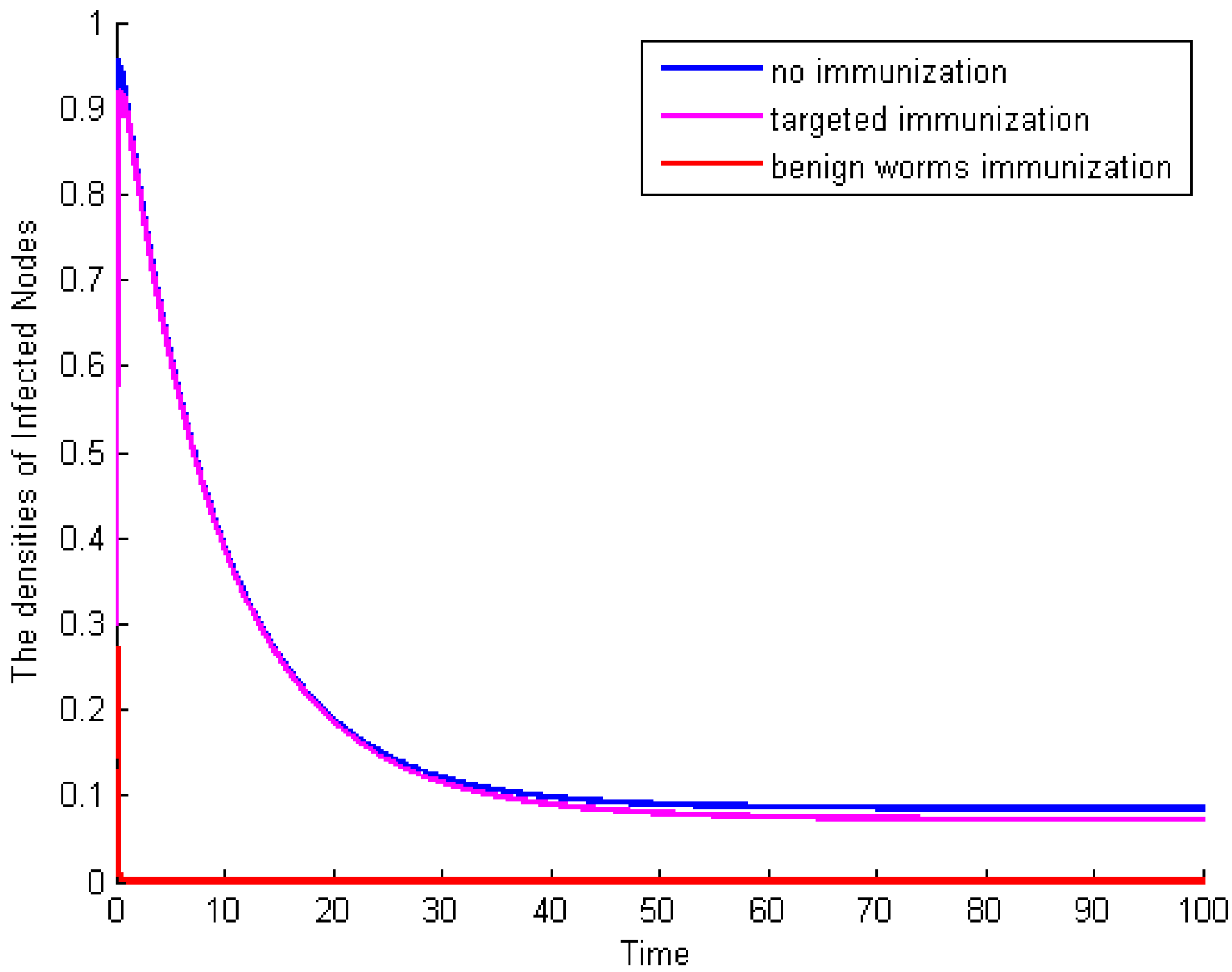
Example 4: Letting $\delta =0.2,{\beta }_1=0.1,{\beta }_2=0.092,{\beta }_3=0.082,{\gamma }_1=0.02,{\gamma }_2=0.01,I_k=0.3,B_k=0.05,$ $V_k=0,1\le k\le \text{Δ}$, Figure 6 shows the time plot of the average densities of malicious infected nodes for different immunization tactics: no immunization, targeted immunization (with $K_1=10,K_2=20,$ $a=0.85,\overline{\eta }=0.087$), and benign worms immunization (with the average infection rate of benign worm is $({\beta }_2+{\beta }_3)/2=0.087$). On purpose, we set the average immunization rates for targeted immunization and benign worms immunization, which are, respectively, 0.087, and then we can make comparison analyses. Figure 6 indicates that, compared to targeted immunization, benign worms immunization has the absolute predominance to control the spread of malicious worms, even though the average infection rate of benign worms is small.

Figure 6. The average densities of malicious infected nodes for different immunization tactics.

Figure 6. The average densities of malicious infected nodes for different immunization tactics.

7. Conclusions

To our knowledge, we are the first to study the complex interactions between benign worms and malicious worms in heterogeneous M2M network. We, respectively, obtain the equilibriums and basic reproduction number of three different models. Meanwhile, we prove that the global dynamics are determined by the threshold value $R_0$. In the absence of birth, death and the treatment effect of users, we obtain the final size formula in different immunization schemes. Our results show that the nodes with higher node degrees are more susceptible to infection than those with lower node degrees. Furthermore, the effects of various immunization schemes are studied. Numerical simulations verify our results. This paper provides a strong theoretical basis to take effective measures to control the large-scale propagation of malicious worms in heterogeneous M2M network. In the future, we are going to incorporate time delay of susceptible and/or infectious computers (malicious infected or benign infected) into the proposed worm propagation models, which will greatly enhance the practicability of our models.

References

- 2015 Symantec Global Internet Security Threat Report. Available online: http://www.symantec.com/security_response (accessed on 9 October 2015).
- Yang, L. Towards the Epidemiological Modeling of Computer Viruses. Discrete Dyn. Nat. Soc. 2012, 245, 348–349. [Google Scholar] [CrossRef]
- Latifi, S.; Srimani, P.K. A new fixed degree regular network for parallel processing. In Proceedings of the Eighth IEEE Symposium on Parallel and Distributed Processing, New Orleans, LA, USA, 23–26 October 1996; pp. 152–159.
- Erdos, P.; Rényi, A. BRandom graphs. Math. Inst. Hung. Acad. Sci. 1960, 5, 17–61. [Google Scholar]
- Amaral, L.A.N.; Scala, A.; Barthelemy, M.; Stanley, H.E. Classes of small-world networks. Proc. Natl. Acad. Sci. (USA) 2000, 97, 11149–11152. [Google Scholar] [CrossRef] [PubMed]
- Anderson, R.M.; May, R.M. Infectious diseases of humans: Dynamics and control. Infect. Dis. Hum. Dyn. Control 1991, 108, 174–175. [Google Scholar]
- Capasso, V.; Serio, G. A generalization of the Kermack-McKendrick deterministic epidemic model. Math. Biosci. 1978, 42, 43–61. [Google Scholar] [CrossRef]
- Zou, C.; Gong, W.; Towsley, D. Code red worm propagation modeling and analysis. In Proceedings of the 9th ACM Conference on Computer and Communications Security, Washington, DC, USA, 17–21 November 2002; pp. 138–147.
- Zou, C.; Gong, W.; Towsley, D. Worm propagation modeling and analysis under dynamic quarantine defense. Workshop Rapid Malcode 2003, 23, 51–60. [Google Scholar]
- Chen, Z.; Gao, L.; Kwiat, K. Modeling the spread of active worms. In Proceedings of the Twenty-Second Annual Joint Conference of the IEEE Computer and Communications (INFOCOM 2003), San Francisco, CA, USA, 30 March–3 April 2003; pp. 1890–1900.
- Mishra, B.K.; Saini, D.K. SEIRS epidemic model with delay for transmission of malicious objects in computer network. Appl. Math. Comput. 2007, 188, 1476–1482. [Google Scholar] [CrossRef]
- Toutonji, O.A.; Yoo, S.M.; Park, M. Stability analysis of VEISV propagation modeling for network worm attack. Appl. Math. Model. 2012, 36, 2751–2761. [Google Scholar] [CrossRef]
- Zhu, Q.; Yang, X.; Yang, L.; Zhang, C. Optimal control of computer virus under a delayed model. Appl. Math. Comput. 2012, 218, 11613–11619. [Google Scholar] [CrossRef]
- Zhu, Q.; Yang, X.; Yang, L.; Zhang, X. A mixing propagation model of computer viruses and countermeasures. Nonlinear Dyn. 2013, 73, 1433–1441. [Google Scholar] [CrossRef]
- Yang, L.; Yang, X.; Zhu, Q.; Wen, L. A computer virus model with graded cure rates. Nonlinear Anal. Real World Appl. 2013, 14, 414–422. [Google Scholar] [CrossRef]
- Hein, D.I.O.; Schwind, D.W.I.M.; König, W. Scale-free networks. Wirtschaftsinformatik 2006, 48, 267–275. [Google Scholar] [CrossRef]
- Liu, J.; Zhang, T. Epidemic spreading of an SEIRS model in scale-free networks. Commun. Nonlinear Sci. Numer. Simul. 2011, 16, 3375–3384. [Google Scholar] [CrossRef]
- Wang, L.; Dai, G. Global Stability of Virus Spreading in Complex Heterogeneous Networks. Siam J. Appl. Math. 2008, 68, 1495–1502. [Google Scholar] [CrossRef]
- Yang, M.; Chen, G.; Fu, X. A modified SIS model with an infective medium on complex networks and its global stability. Physica A 2011, 390, 2408–2413. [Google Scholar] [CrossRef]
- Zhang, H.; Fu, X. Spreading of epidemics on scale-free networks with nonlinear infectivity. Nonlinear Anal. 2009, 70, 3273–3278. [Google Scholar] [CrossRef]
- Olinky, R.; Stone, L. Unexpected epidemic thresholds in heterogeneous networks: The role of disease transmission. Phys. Rev. E 2004, 70, 193–204. [Google Scholar] [CrossRef]
- Li, C.-H.; Tsai, C.-C.; Yang, S.-Y. Analysis of epidemic spreading of an SIRS model in complex heterogeneous networks. Commun. Nonlinear Sci. Numer. Simul. 2014, 19, 1042–1054. [Google Scholar] [CrossRef]
- Small, M. Staged progression model for epidemic spread on homogeneous and heterogeneous networks. J. Syst. Sci. Complex. 2011, 24, 619–630. [Google Scholar]
- Gan, C.; Yang, X.; Liu, W.; Zhu, Q.; Jin, J.; He, L. Propagation of computer virus both across the Internet and external computers: A complex-network approach. Commun. Nonlinear Sci. Numer. Simul. 2014, 19, 2785–2792. [Google Scholar] [CrossRef]
- Fadlullah, Z.M.; Fouda, M.M.; Kato, N.; Takeuchi, A.; Iwasaki, N.; Nozaki, Y. Toward intelligent machine-to-machine communications in smart grid. IEEE Commun. Mag. 2011, 49, 60–65. [Google Scholar] [CrossRef]
- Zhou, H.; Wen, Y.; Zhao, H. Modeling and analysis of active benign worms and hybrid benign worms containing the spread of worms. In Proceedings of the Sixth IEEE International Conference on Networking (ICN '07), Saint Luce, Martinique, 22–28 April 2007; p. 65.
- Ma, J.; Chen, Z.; Wu, W.; Zheng, R.; Liu, J. Influences of Removable Devices on the Anti-Threat Model: Dynamic Analysis and Control Strategies. Information 2015, 6, 536–549. [Google Scholar] [CrossRef]
- Wang, F.; Yang, Y.; Zhang, Y.; Ma, J. Stability analysis of the interaction between malicious and benign worms. In Future Computer and Information Technology; Zheng, D., Zhang, L., Eds.; WIT Press: Southampton, UK, 2013; pp. 217–225. [Google Scholar]
- Zheng, X.; Li, T.; Fang, Y. Strategy of fast and light-load cloud-based proactive benign worm countermeasure technology to contain worm propagation. J. Supercomput. 2012, 62, 1451–1479. [Google Scholar] [CrossRef]
- Fan, X.; Xiang, Y. Modeling the Propagation Process of Topology-Aware Worms: An Innovative Logic Matrix Formulation. In Proceedings of the Sixth IFIP International Conference on Network and Parallel Computing (NPC '09), Gold Coast, Australia, 19–21 October 2009; pp. 182–189.
- Wang, Y.; Wen, S.; Cesare, S.; Zhou, W.; Xiang, Y. The Microcosmic Model of Worm Propagation. Comput. J. 2011, 54, 1700–1720. [Google Scholar] [CrossRef]
- Fan, X.; Xiang, Y. Modeling the propagation of Peer-to-Peer worms. Future Gener. Comput. Syst. 2010, 26, 1433–1443. [Google Scholar] [CrossRef]
- Fan, X.; Xiang, Y. Modeling the propagation of Peer-to-Peer worms under quarantine. In Proceedings of the 2010 IEEE Network Operations and Management Symposium (NOMS), Osaka, Japan, 19–23 April 2010; pp. 942–945.
- Fan, X.; Xiang, Y. Propagation Modeling of Peer-to-Peer Worms. In Proceedings of the IEEE 24th International Conference on Advanced Information Networking and Applications (AINA), Perth, Australia, 20–23 April 2010; pp. 1128–1135.
- Wang, Y.; Wen, S.; Xiang, Y. Modeling worms propagation on probability. In Proceedings of the IEEE 5th International Conference on Network and System Security (NSS), Milan, Italy, 6–8 September 2011; pp. 49–56.
- Faloutsos, M.; Faloutsos, P.; Faloutsos, C. On power-law relationships of the Internet topology. Acm Sigcomm Comput. Commun. Rev. 1999, 29, 251–262. [Google Scholar] [CrossRef]
- Jin, Z.; Zhang, J.; Song, L.; Sun, G.; Kan, J.; Zhu, H. Modelling and analysis of influenza A (H1N1) on networks. BMC Public Health 2011, 11. [Google Scholar] [CrossRef]
- Diekmann, O.; Heesterbeek, J.A.; Ja, M. On the definition and the computation of the basic reproduction ratio R0 in models for infectious diseases in heterogeneous populations. J. Math. Biol. 1990, 28, 365–382. [Google Scholar] [CrossRef] [PubMed]
- Heffernan, J.M.; Smith, R.J.; Wahl, L.M. Perspectives on the basic reproductive ratio. J. R. Soc. Interface 2005, 2, 281–293. [Google Scholar] [CrossRef] [PubMed]
- Lasalle, J.P. The Stability of Dynamical Systems. Reg. Conf. 1976, 40, 1096–1105. [Google Scholar]
© 2015 by the authors; licensee MDPI, Basel, Switzerland. This article is an open access article distributed under the terms and conditions of the Creative Commons Attribution license (http://creativecommons.org/licenses/by/4.0/).