Expert Refined Topic Models to Edit Topic Clusters in Image Analysis Applied to Welding Engineering

Abstract

This paper proposes a new method to generate edited topics or clusters to analyze images for prioritizing quality issues. The approach is associated with a new way for subject matter experts to edit the cluster definitions by “zapping” or “boosting” pixels. We refer to the information entered by users or experts as “high-level” data and we are apparently the first to allow in our model for the possibility of errors coming from the experts. The collapsed Gibbs sampler is proposed that permits efficient processing for datasets involving tens of thousands of records. Numerical examples illustrate the benefits of the high-level data related to improving accuracy measured by Kullback–Leibler (KL) distance. The numerical examples include a Tungsten inert gas example from the literature. In addition, a novel laser aluminum alloy image application illustrates the assignment of welds to groups that correspond to part conformance standards.

1. Introduction

Clustering is an informatics technique that allows practitioners to focus attention on a few important factors in a process. In clustering, the analyst takes unsupervised or untagged data and divides it into what are intended to be intuitive groupings. Then, knowledge is gained about the whole dataset or “corpus” and any new items can be automatically assigned to groups. As a result, clustering can provide a data-driven prioritization for quality issues relevant to allocating limited attention and resources. Informatics professionals are asked now more than ever to be versant in using the information technology revolution [1,2,3]. This revolution exposed practitioners to large databases of images (and texts) that provided insights into quality issues. Practitioner might easily create clustering or logistic regression models using the rating field. Yet, the practitioner generally has no systematic technique for analyzing the freestyle text or image. This is true even while the text or image clearly contains much relevant information for causal analysis [4,5].

This article proposes methods with sufficient generality to provide the ability to apply the analysis either for images or texts. Each image (or record) could correspond to more than a single quality issue. For example, one part of a weld image might include nonconformity at the same time reveals another type of nonconformity. In addition, it might be too expensive to go through all the images (or documents), to identify the quality issues manually. The purpose of this article is to propose a new way to identify quality issues combined with different images (or texts) by generating clustering charts to prioritize quality issues. For example, if the engineers knew that type 1 defects were much more common than the other types, they could focus on the techniques relevant to type 1 for quality improvement and address the most important issues of that type. This new method will require relatively little effort from practitioners compared with manually tagging all or a large fraction of the data.

Even while the information technology revolution is exposing practitioners to new types of challenges it is also making some relevant estimation methods like Bayesian analysis easier [6,7,8,9]. One aspect that many Bayesian applications have in common is that they do not apply informative prior distributions. This is presumably because, in all these cases, the relevant practitioners did not have sufficient knowledge before analysis that they could confidently apply to make the derived models more accurate. The phrase “supervised” data analysis refers to the case in which all the data used for analysis has been analyzed by subject matter experts (SMEs) and categorized into classes by cause or type. Past analyses of text or image data in quality contexts have focused on supervised data analyses [10,11]. Yet, more generally perhaps, datasets are sufficiently large that having personnel read or observe all or even a significant fraction of the articles or images and categorize them into types is prohibitively expensive. Apley and Lee [12] developed a framework for integrating on-line and off-line data which is also presented in this article. This framework did not include new types and convenient types of data. Here, we are seeking to have the data presented in different forms.

The approach proposed in this paper is apparently the first to model replication and other errors in both high-level expert and “low-level” data for unstructured multi-field text or image modeling for image analysis. Allen, Xiong and Afful-Dadzie [4] did this for text data. The practical benefit that we seek is to permit the user to edit the cluster or topic definitions easily. In general, Bayesian mixture models provide clusters with interpretable meaning and are generalizations of latent semantic indexing approaches [13]. The Latent Dirichlet Allocation (LDA) method [13] has received a lot of attention because the cluster definitions derived often seem interpretable. Yet, these definitions may seem inaccurate and disagree with expert judgement. Most recently, many researchers have further refined Bayesian mixture models to make the results even more interpretable and predictive [14,15,16,17,18]. This research has generally caused the complexity of the models to grow together with the number of estimated parameters. The approach taken here is to use a relatively simple formulation and attempt to mitigate the misspecification issues by permitting user interaction through the high-level data.

To generate clustering models to analyze image data, we must identify clusters definitions which is the most challenging step, tally the total proportions of all the images associated with each cluster, sort the tallies and bar chart the results. Another objective we have for this article is to compare the proposed clustering methods with alternatives methods that have been used before. This follows because those methods require that the cluster definitions are pre-defined, all pixels in each image relate to a single cluster, and a “training set” of images have been pre-tagged or supervised [19,20,21]. For two simulated numerical examples, we compare the proposed clustering methods with three relevant alternatives: Latent Dirichlet Allocation [13,22,23], “fuzzy c means” clustering methods [24,25] and pre-processing using principle components analysis followed by fuzzy c means clustering [26]. Apparently, comparisons of a similar scope do not appear in the image analysis literature which generally focuses on the goal of retrieving relevant documents. Our research here applies the existing results for text analysis [4]. To generate helpful prioritizations, we need the estimated topic definitions and proportions to be accurate. Therefore, we also propose new measures of model accuracy relevant to our goals for image analysis.

Next section, we describe the laser welding image problem that motivates the Expert Refined Topic (ERT) modeling methods for image analysis. The motivation relates to the issue that none of the topics or clusters identified directly corresponds to the issues defined in the American National Standard Institute (ANSI) conformance standards.

Motivating Problem: Laser Welding

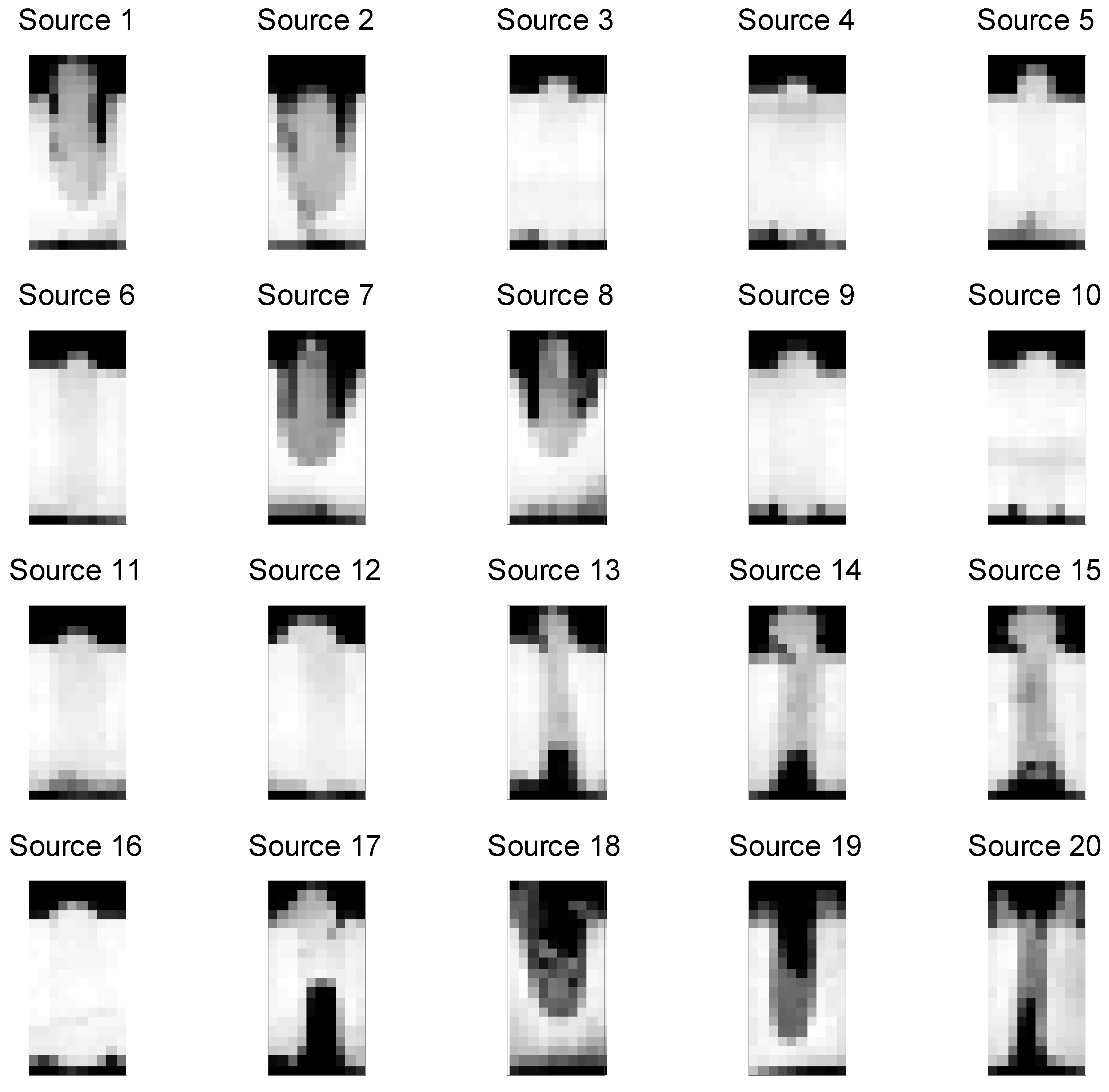
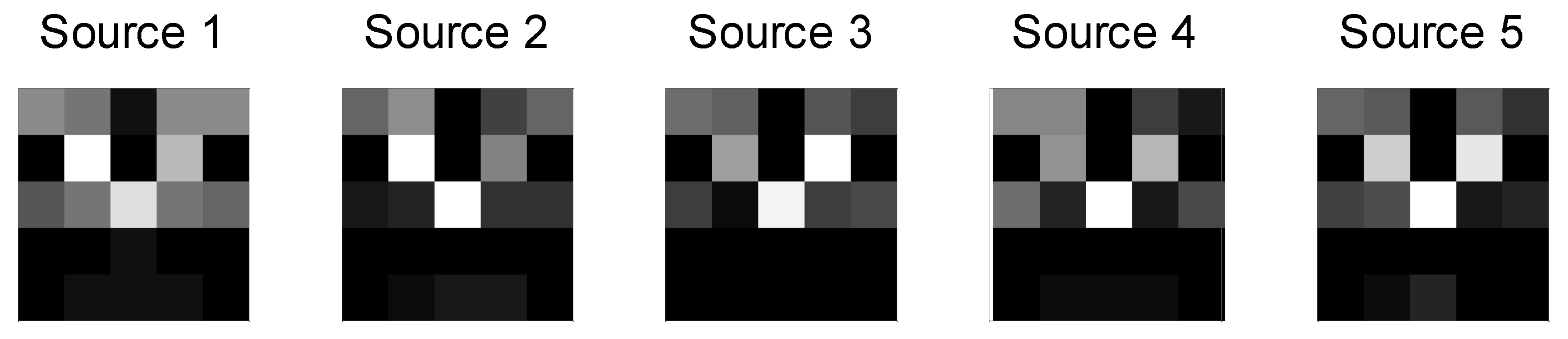
Many manufacturing processes involve images used to evaluate the conformance of parts to standards [6,27,28]. Figure 1 shows digital images from 20 laser aluminum alloy parts, which were sectioned and photographed. The first image (Source 1) can be represented as a vector of pixel numbers with added counts for the darker pictures. This is given in

Table 1. (a) Data for the first low-level image; (b) 25 high-level data points with zaps with one million (M) effective trials and boosts.

(a)
Source 1
1	1	1	1	1	1	1	1	3	3
3	3	3	6	6	6	6	6	6	6
7	7	7	7	7	7	7	7	7	7
7	7	7	7	7	8	8	8	8	8
8	8	10	11	13	13	13	13	13	13
13	13	13	13	13	13	13	14	15	16
16	16	16	16	16	16	16	17	17	17
17	17	17	17	17	17	17	17	18	18
18	18	18	18	18	20	21	21	21	21
21	21	21	21	23	23	23	23	23	23
(b)
Topic		Word (c)			Trials (N)			x
1		13			1M			0
1		3			1M			0
1		8			1M			0
1		18			1M			0
1		23			1M			0
2		1			1M			0
2		6			1M			0
2		16			1M			0
2		21			1M			0
2		7			1M			0
2		17			1M			0
3		10			2			2
3		15			2			2
3		20			2			2
3		1			1M			0
3		6			1M			0
3		7			1M			0
3		16			1M			0
3		17			1M			0
3		21			1M			0
3		13			1M			0
3		3			1M			0
3		8			1M			0
3		18			1M			0
3		23			1M			0

(a). This “bag of words” representation is common to topic models but has drawbacks including the document lengths being related to the number of distinct levels of grayscale [13]. Table 1(b) includes the inputs from our methods which are described in Section 4. In this example, the number of images is small enough such that supervision of all images manually is not expensive. In addition, generating the image data of cut sections of the welds is expensive because the process is destructive, i.e., the sectioned parts cannot be sold. Generally, manufacturing situations that involve nondestructive evaluation can easily generate thousands of images or more. In these situations, human supervision of even a substantial fraction of these images is prohibitively expensive. Our problem statement is to create topic definitions and an automatic system that can cluster items (weld images) into groups that conform to pre-known categories while spanning the set of actual items. We seek to do this with a reasonable request of information from the welding engineers involved.

In addition, in Figure 1, the images may seem blurry. This follows because they are 20 × 10 = 200 pixels because it was judged that such simple images are sufficient for establishing conformance and are easier to store and process than higher resolution images. We will discuss the related issues of resolution and gray scale bit selection after the methods have been introduced. In the next section, we review the methods associated with Latent Dirichlet Allocation (LDA) [13].

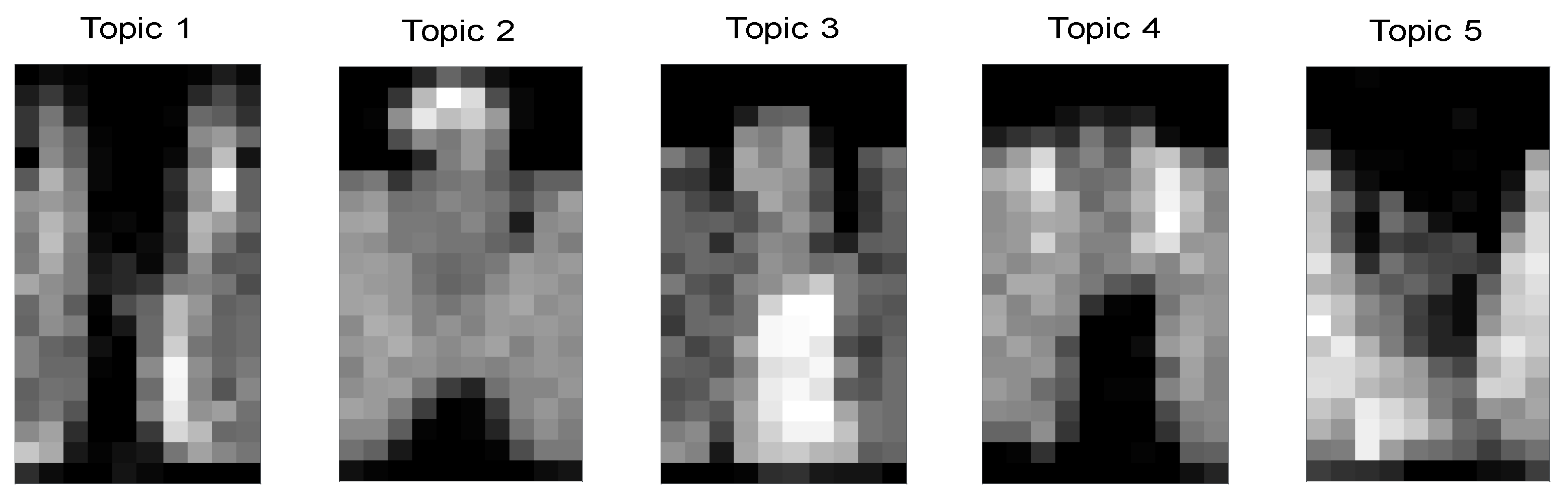
LDA is perhaps the most widely cited method relevant to unsupervised image processing. The cluster or “topic” definitions identified by LDA can themselves be represented as images. They are defined formally by the posterior means for the pixel or “word” probabilities associated with each topic. Figure 2 shows the posterior mean topic definitions from applying 3000 iterations of collapsed Gibbs sampling using our own C++ implementation. The topic definitions are probabilities that each pixel would be selected in a random draw or word. The fact that they can be interpreted themselves as images is a positive properties of topic models such as LDA.

At present, there are many methods to determine the number of topics in the fitted model [29,30,31,32,33]. Appendix B describes the selection of five topics for this problem. Figure 3 illustrates the most relevant international American National Standard Institute/American Welding Society (ANSI/AWS) conformance issues for the relevant type of aluminum alloy pipe welds [30]. These were hand drawn but they are quite standard and illustrate the issues an arc welding quality inspector might look for in examining images from a sectioned part.

If it were possible to have the topic definitions correspond closely with these known conformance issues, then the resulting model could not only assign the probability that welds are conforming but also provide the probabilities of specific issues applying. In addition, the working vocabulary of welding engineers including “undercut”, “penetration” and “stickout” could be engaged to enhance interpretability [34]. The primary purpose of this article is to propose methods that provide recourse for users to shape the topics directly without tagging individual images.

Section 2 describes the related works. In Section 3, we describe the notation and review the Latent Dirichlet Allocation methods whose generalization forms the basis of ERT models, which are then proposed for image analysis. The ERT model application involves a step in which “handles” are applied using thought experiments to generate high-level data in Section 4.

Then we describe the “collapsed” Gibbs sampling formulation, which permits the exploration of databases involving thousands of images or documents. The proposed formulation is exact in certain cases that we describe and approximate in others, with details provided in Appendix A. In Section 5, two numerical examples illustrate the benefits for cases in which the ground truth is known. In Section 6, we illustrate the potential value of the method in the context of a real-world, laser welding image application and conclude with a brief discussion of the balance between high-level and ordinary data in modeling in Section 7.

2. Related Works

Latent Dirichlet Allocation (LDA) was proposed by [13]. It is the most cited method for clustering unsupervised images or text documents perhaps because of its relative simplicity and because the resulting cluster or topic definitions are often interpretable [29]. The LDA method is simply to fit a complicated seeming distribution to data using a distribution fitting method. This clustering method has a wide variety of applications including grouping the activities of daily life [31].

In the original LDA article, Blei et al. focused on an approximate maximum likelihood estimation method. They also introduced a method to determine the number of clusters or topics based on the so-called “perplexity” metric. This metric gives an approximate indication of how well the distribution predicts a held-out test sample. Other methods for determining the number of topics have been subsequently introduced. A general discussion suggest that perplexity is still relevant [32] for cases without any tagged data. One automatic alternative to perplexity-based plotting is argued to be faster in analyst time but approximately equivalently accurate [33]. Further alternative entropy-based measures to perplexity are proposed for cases in which perplexity does not achieve a minimum or the elbow curves are not clear [34]. Note that in our primary example, we do not have tagged data and our perplexity does achieve a minimum value. Therefore, we apply perplexity plot-based model determination.

3. Notation

In our notation, the ordinary or low-level data are the pixels indices in each image or document. Specifically, $w_{d,n}$ represents a so-called word in an image or document for d = 1, …, D and for n = 1, …, N_d. Therefore, “D” is the number of images or documents and “N_d” is the number of words in the dth document. We use the term “documents” to describe the low-level data instead of images because the images are converted to un-ordered listings of pixel indices before there are analyzed. This means that we convert 2D images into 1D vectors of pixel indices. We use 8-bit gray scale which runs from 0 to 255. The higher the gray scale the more repeated pixel indices which are the words in the documents. Table 1(a) provides an example of how the images are related to words in the documents. This example applies to the relatively simple face image example in Section 5, which only has 25 pixels in each image. The laser welding source images in Figure 1 all have over 15,000 words, i.e., N_d > 15,000 for d = 1, …, 20.

A random variable is the multinomial or cluster or topic assignment, $z_{d,n}$, for $w_{d,n}$. The T-dimensional random vector ${\theta }_d$ represents the probabilities a randomly selected pixel in document d is assigned to each of the T topics or clusters. The parameter “WC” represents the number or pixels or words in the dictionary. For example, in our laser welding study there are D = 20 images each with 200 pixels. Therefore, WC = 200. The WC-dimensional random vector ${\varphi }_t$ represents the probability that randomly selected words are assigned to each pixel in the topic indexed by t = 1, …, T. The posterior mean of ${\varphi }_t$ for each pixel is generally used to define the topics as has been shown in Figure 2. The prior parameters $\alpha$ and $\beta$ are usually scalars in that all documents and all pixels are initially treated equally. Generally, low values or “diffuse priors” are applied such that only a small amount of shrinkage is applied, and adjustments are made on a case-by-case basis [35].

The key purpose of this article is to study the effects of our proposed high-level data on image analysis applications. The high-level data derives from imagined counts $x_{t,c}$ from binomial thought experiments with possible values as high as $N_{t,c}$. The elicitation question is, “Out of $N_{t,c}$ random draws relating to topic t, how many times would pixel c occur?” If $x_{t,c}=0$ and ${\mathsf{\Delta }}_{t,c}=N_{t,c}-x_{t,c}\gg 0$, the user or expert is zapping the pixel in that image. This is equivalent to erasing that pixel in the topic. If ${\mathsf{\Delta }}_{t,c}=0$ and $N_{t,c}>0$, then the user or expert is boosting or affirming that pixel in that topic.

Latent Dirichlet Allocation

With these parameter definitions, LDA is defined by the following joint posterior distribution function proportional condition:

$$\begin{array}{cc}\hfill P\left(w,z,\theta ,\varphi |\alpha ,\beta \right)& =P\left(\theta |\alpha \right)P\left(z|\theta \right)P\left(\varphi |\beta \right)P\left(w|z,\varphi \right)\hfill \\ & \propto {\displaystyle {\displaystyle \prod }_{d=1}^D}Dir\left({\theta }_d|\alpha \right)\times {\displaystyle {\displaystyle \prod }_{d=1}^D}{\displaystyle {\displaystyle \prod }_{n=1}^{N_d}}Mult\left(z_{d,n}|{\theta }_d\right)\times {\displaystyle {\displaystyle \prod }_{t=1}^T}Dir\left({\varphi }_t|\beta \right)\hfill \\ & \times {\displaystyle {\displaystyle \prod }_{d=1}^D}{\displaystyle {\displaystyle \prod }_{n=1}^{N_d}}Mult\left(w_{d,n}|{\varphi }_{z_{d,n}}\right)\hfill \end{array}$$

(1)

where

$$Dir\left(\theta |\alpha \right)=\frac{1}{B\left(\alpha \right)} {\displaystyle \prod }_{t=1}^{\left|\alpha \right|}{\theta }^{{\alpha }_t-1}$$

(2)

and

$$Mult\left(x|\theta ,n\right)=\frac{n!}{{\prod }_{k=1}^K{x}_k!}{\displaystyle \prod }_{k=1}^K{\theta }_k^{x_k} \to Mult\left(x|\theta ,1\right)={\displaystyle \prod }_{k=1}^K{\theta }_k^{x_k}$$

(3)

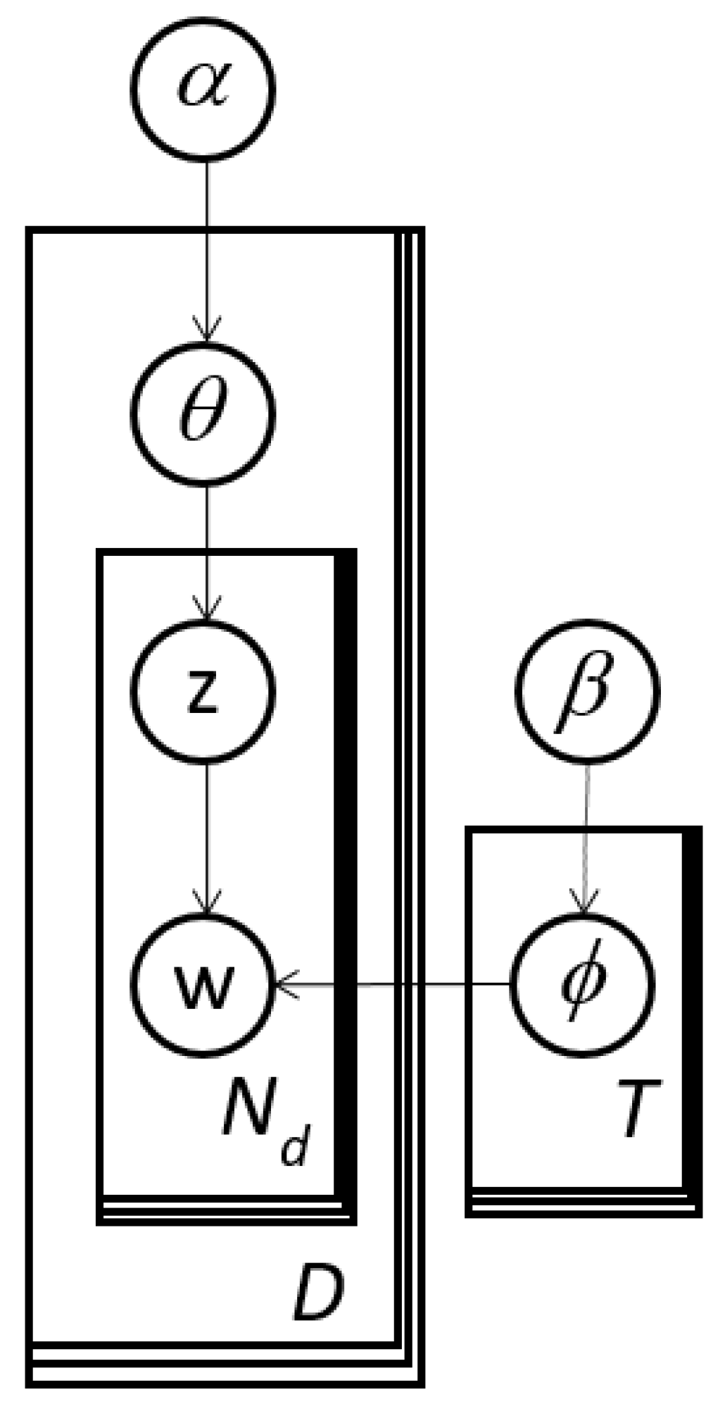
The graphical model in Figure 4 summarizes the conditional relationships between the variables in the LDA model. The rectangles indicate the number of elements in each random vector or matrix. For example, the random matrices z and w have N_d elements for each of the D images as mentioned previously.

Griffiths and Steyvers [35] invented the so-called collapsed Gibbs updating function which permits Gibbs sampling for estimation of the proportionality constant in Equation (1) via only sampling the $z_{d,n}$ random variables. The other random variables ($\theta$ and $\varphi$) are effectively “integrated out” and their posterior means are estimated after thousands of iterations as functions of the sampled $z_{d,n}$ values. This approach is many times faster than ordinary Gibbs sampling and can avoid the need for abandoning the Bayesian model formulation.

To apply collapsed Gibbs sampling for LDA, we define the indexing matrix C_t,d,c, which is the number of times word c is assigned to topic t in document d, where t is topic index, d is the document index and c is the word index, as the following:

$$C_{t,d,c}={\displaystyle \sum }_{j=1}^{N_d}I\left(z_{d,j}=t \& w_{d,j}=c\right)$$

(4)

where I() is an indicator function: 1 if the condition is true and 0 if false. Then, the topic-document count matrix is:

$$C_{t,*,c}={\displaystyle \sum }_{d=1}^D{C}_{t,d,c}$$

(5)

and the topic-word count matrix is:

$$C_{t,d,*}={\displaystyle \sum }_{c=1}^{WC}{C}_{t,d,c}$$

(6)

We further define q_t,c $={\beta }_c+C_{t,*,c}$ and $q_{t,c}^{-\left(t,c\right)}={\beta }_c+C_{t, *,c}^{-\left(t,c\right)}$. The collapsed Gibbs multinomial probabilities for sampling the topic $z_{a,b}$ for word b in document a are:

$$\begin{array}{c}P\left(z_{a,b}|z_{-\left(a,b\right)}, w, \alpha ,\beta \right)\propto P\left(z_{a,b}|z_{-\left(a,b\right)}, w, \alpha ,\beta \right)\hfill \\ \propto \left(C_{z_{a,b}, a,*}^{-\left(a,b\right)}+{\alpha }_{z_{a,b}}\right)\times \frac{q_{z_{a,b},w_{a,b}}^{-\left(a,b\right)}}{{{\displaystyle \sum }}_{j=1}^{WC}{q}_{z_{a,b},j}^{-\left(a,b\right)}}\mathrm{for}{z}_{a,b}=1,\dots ,\mathrm{T}.\hfill \end{array}$$

(7)

The posterior mean for the topic definition probabilities,${\varphi }_{t,c}$, are:

$$E\left({\varphi }_{t,c}|t,N,x,w,\beta \right)=\frac{q_{t,c}}{{\sum }_{j=1}^{WC}{q}_{t,j}}\mathrm{for}t=1,\dots ,T\mathrm{and}c=1,\dots ,\mathrm{WC}.$$

(8)

The collapsed Gibbs estimation process begins with a uniform random sampling of the $z_{a,b}$ for every document, a, and word, b, and then continues with repeated applications of multinomial sampling based on Equation (7), again for all a and b pairs. After a sufficient number of complete replications, the $z_{a,b}$ assignments approximately stabilize and the posterior mean probabilities are estimated using Equation (8). Replication sufficiency can be established by monitoring the approximate stability of the estimated parameters, e.g., in Equation (8). The iterations before the establishment of stability may be called the “burn-in” period. After convergence, the probabilities can then be converted into images by linear scaling based on the high and low values for all pixels so that all resulting values range between 0 and 255 and then rounding down to obtain the grayscale images, e.g., see Figure 2.

Topic modeling methods including those based on Gibbs sampling have been criticized for being unstable [36], i.e., they produce different groupings on subsequent runs even for the same data. Some measure stability and directly try to minimize cross-run differences based on established stability measures [37]. Others propose innovative stability or similarity measurements [38]. Still others propose both innovate stability measures and methods to maximize stability [39]. An objective of the methods described in the next section is to make the final results more repeatable and accurate by focusing directly on accuracy, i.e., increased stability is a by-product. The numerical study in Section 5 seeks to demonstrate that the proposed methods are both more stable and more accurate than previous methods.

4. Methods

Widely acknowledged principles for modeling and automation include that the models should be both “observable” so that the users can see how they operate and “directable” so that users can make adjustments on a case-by-case basis [40]. We argue that topic models are popular partly because they are simpler and, therefore, more observable than alternative models, which might include expert systems having thousands of ad hoc, case-specific rules. Yet, the only “directability” in topics models comes through the prior parameters α and β. Specifically, adjustments to α and β only control the degree of posterior uniformity in the document-topic probabilities and the degree of uniformity of the topic-word probabilities, respectively. Therefore, α and β are merely Bayesian shrinkage parameters.

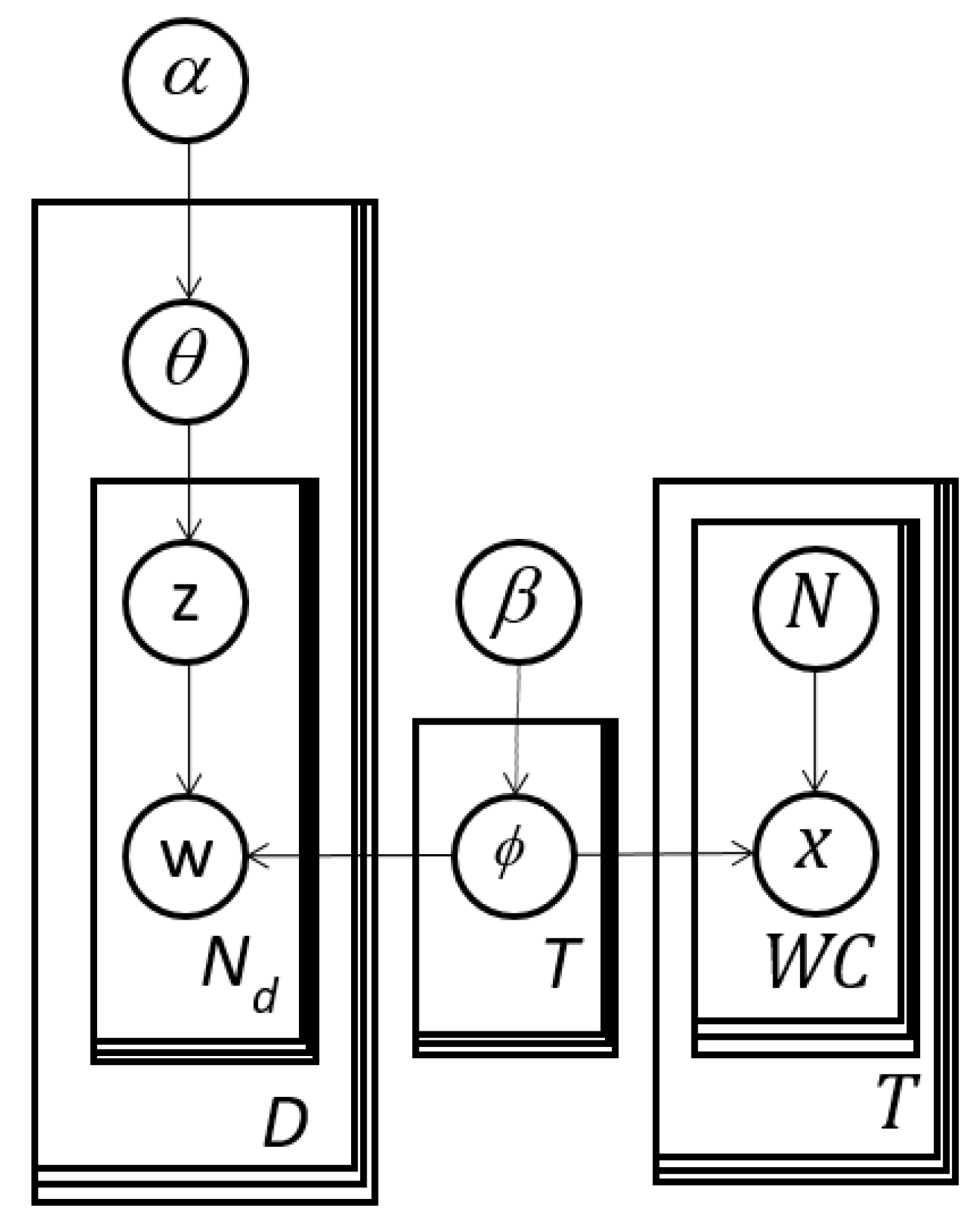
We propose for image analysis the subject matter expert refined topic (ERT) model in Figure 5 to make the LDA topic model more directable. The left-hand-side is identical to LDA in Figure 4, which has multinomial response data, w. The right-hand-side is new and begins with the arrow from ϕ to x. This portion introduces binomially distributed response data, $x_{t,c}$ for t = 1, …, T and c = 1, …, WC. The $x_{t,c}$ represent the number of times for a given topic, t, word c is selected in $N_{t,c}$ trials. Therefore, $N_{t,c}$ is a sample size for thought experts.

Like LDA, ERT models are merely distributions to be fit to data. The usual data points are assumed to be random (multinomial) responses (ws) which are part of the LDA “wing” (left-hand-side of Figure 5). The inputs from the experts (or just users) are random counts (xs) from imaged “thought” experiments on the right-hand-side (right wing) of Figure 5.

In our examples, we use $N_{t,c}$ = 1M for cases when the expert or user is confident that they want to remove a word (“zap”). Smaller sizes, e.g., $N_{t,c}$ = 1000, might subjectively indicate less confidence or weight in the expert data. In our preliminary robustness studies, sample sizes below 1M often had surprisingly little effect for zapping. Note also that the choice of $N_{t,c}$ in the model is arbitrary and many combinations of topics t and words c can have $N_{t,c}=0$.

We refer to the right-hand-side portions in Figure 4 (the rectangles including N and x) as handles because they permit users to interact with the model in a novel way in analogy to using a carrying appendage on a pot. These experiments are “designed” because the analyst can plan and direct the data collection. These binomial thought experiments have relatively high leverage on specific latent variables, i.e., ϕ. We propose that users can apply this model in two or more stages. After initially applying ordinary LDA, the user can study the results and then gather data from experiments involving potentially subject matter experts (SMEs) leading to Expert Refined Topic (ERT) models or Subject Matter Expert Refined Topic (SMERT) models. Note that a similar handle could be added to any other topic model with a similarly defined topic definition matrix, ϕ.

The so-called “latency experiments” [4] could be literal as having the expert create prototype images for each topic and then extracting the binomial counts from these images. Alternatively, the experiments could be simple thought experiments, i.e., out of several trials, how many draws would you expect to result in a certain pixel image being derived? One difference than makes ERT models different for images as compared with text [4] is that zapping is essentially an “eraser” for the topic definitions. This could even be accomplished using eraser icons on touch screens.

As an example, consider that an expert might be evaluating topic 1 in Figure 2. The expert might conclude that topic t = 1 should be transformed to resemble topic 2 (undercut) in Figure 3. The expert might focus on pixel c = 22, which is in the middle top. The expert concludes that in N_1,22 = 1 million samples from the topic (trials), the topic index should be found x_1,22 = 0 times, i.e., the pixel should be black because it is in the middle of the cavity. We have found in our numerical work that the boosting and zapping tables need to address a large fraction of the words in each topic to be effective, i.e., little missing data. Otherwise, the estimation process can shift the topic numbers to avoid the effects of supervision.

The Collapsed Gibbs Sampler

The joint posterior distribution that defines the ERT model has proportionality given by:

$$\begin{array}{cc}P\left(z,w,x,\theta ,\varphi |N,\alpha ,\beta \right)\hfill & \\ & \hfill \propto {\displaystyle {\displaystyle \prod }_{d=1}^D}Dir\left({\theta }_d|\alpha \right)\times {\displaystyle {\displaystyle \prod }_{d=1}^D}{\displaystyle {\displaystyle \prod }_{n=1}^{N_d}}Mult\left(z_{d,n}|{\theta }_d\right)\times {\displaystyle {\displaystyle \prod }_{t=1}^T}Dir\left({\varphi }_t|\beta \right)\\ & \times {\displaystyle {\displaystyle \prod }_{d=1}^D}{\displaystyle {\displaystyle \prod }_{n=1}^{N_d}}Mult\left(w_{d,n}|{\varphi }_{z_{d,n}}\right)\times {\displaystyle {\displaystyle \prod }_{t=1}^T}{\displaystyle {\displaystyle \prod }_{c=1}^{WC}}Bin\left(x_{t,c}|N_{t,c},{\varphi }_{t,c}\right)\hfill \end{array}$$

(9)

where $z,w,x,\theta ,\varphi$ and N are vectors defining assignments for all words in all documents. The binomial distribution function is:

$$Bin\left(x_{t,c}|N_{t,c},{\varphi }_{t,c}\right)=\left(\begin{array}{c}{N}_{t,c}\\ x_{t,c}\end{array}\right){\varphi }_{t,c}^{x_{t,c}}{\left(1-{\varphi }_{t,c}\right)}^{N_{t,c}-x_{t,c}}$$

(10)

Here, we generalize our definitions such that q_t,c $={\beta }_c+C_{t,*,c}+x_{t,c}$ and we also define ${\mathsf{\Delta }}_{t,c}=N_{t,c}-x_{t,c}$. Further, we define the set S to include combinations of t and c such that ${\mathsf{\Delta }}_{t,c}$ > 0 in the high-level data (i.e., the zaps). Appendix A builds on previous research [4,41,42]. Appendix A describes the derivation of the following collapsed Gibbs updating function for the combinations with $z_{a,b}$ and $w_{a,b}\in S$:

$$\begin{array}{cc}P\left(z_{a,b}|z_{-\left(a,b\right)}, w, \alpha ,\beta \right)\hfill & \propto P\left(w_{a,b}|z_{-\left(a,b\right)},w_{-\left(a,b\right)},\beta \right)\hfill \\ & \propto \left(C_{z_{a,b}, a,*}^{-\left(a,b\right)}+{\alpha }_{z_{a,b}}\right)\times \frac{q_{z_{a,b},w_{a,b}}^{-\left(a,b\right)}}{{\mathsf{\Delta }}_{z_{a,b},w_{a,b}}+{\sum }_{j=1}^{WC}\left(q_{z_{a,b},j}^{-\left(a,b\right)}\right)}\hfill \end{array}$$

(11)

For, $z_{a,b}$ and $w_{a,b}\notin S$ the updating function is:

$$\begin{array}{cc}P\left(z_{a,b}|z_{-\left(a,b\right)}, w, \alpha ,\beta \right)\hfill & \propto P\left(w_{a,b}|z_{-\left(a,b\right)},w_{-\left(a,b\right)},\beta \right)\hfill \\ & \propto \left(C_{z_{a,b}, a,*}^{-\left(a,b\right)}+{\alpha }_{z_{a,b}}\right)\times \frac{q_{z_{a,b},w_{a,b}}^{-\left(a,b\right)}}{{\sum }_{i=1}^{WC}\left(q_{z_{a,b},i}^{-\left(a,b\right)}\right)-{\sum }_{j\in S}\left(q_{z_{a,b},j}^{-\left(a,b\right)}\right)}\hfill \\ & \times \left(1-{{\displaystyle \sum }}_{k\in S}\left(\frac{q_{z_{a,b},k}^{-\left(a,b\right)}}{{\mathsf{\Delta }}_{z_{a,b},k}+{\sum }_{i=1}^{WC}\left(q_{z_{a,b},i}^{-\left(a,b\right)}\right)}\right)\right)\hfill \end{array}$$

(12)

The posterior mean for the combinations with t and $c\in S$ is:

$$E\left({\varphi }_{t,c}|t,N,x,w,\beta \right)=\frac{q_{t,c}}{{\mathsf{\Delta }}_{t,c}+{\sum }_{j=1}^{WC}{q}_{t,j}}$$

(13)

For t and $c\notin S$ we have:

$$E\left({\varphi }_{t,c}|t,N,x,w,\beta \right)=\frac{q_{t,c}}{{\sum }_{j=1}^{WC}{q}_{t,j}-{\sum }_{j\in S}{q}_{t,j}}\left(1-{\sum }_{k\in S}\left(\frac{q_{t,k}}{{\mathsf{\Delta }}_{t,k}+{\sum }_{j=1}^{WC}\left(q_{t,j}\right)}\right)\right)$$

(14)

Note that if $N_{t,c}$ = 0 for all t = 1, …, T and c = 1, …, WC, then Equation (12) reduces to Equation (7) and Equation (14) reduces to Equation (8). As is clear from Figure 4 and Figure 5, the ERT model is a generalization of the LDA model. In addition, as clarified in Appendix A, Equations (11)–(14) are approximate for cases in which the set S contains more than a single pixel in each topic. Yet, the numerical investigations that follow and the computational experiment in Appendix C indicate that the quality of the approximation is often acceptable.

Note that the pseudocode for ERT sampling is identical to LDA sampling pseudocode with Equation (12) replacing Equation (7). Therefore, the scaling of computational costs with the number of pixel gray scale values follows because the document lengths grow proportionally (see Table 1(a)). Boosting minimally affects the computation since it does not relate to the set S. Zaps, however, require the calculation of two additional sums, which directly inflate the core costs linearly in the number of zapped words.

In our computational studies, we have found that each iteration is slower because of the associated sums in Equation (7). Yet, the burn-in period required is less, e.g., 300 iterations instead of 500. Intuitively, burn-in is faster because the high-level data anchors the topic definitions.

5. Results: Examples

In this section, three examples are described for which the first two have the true model or “ground truth” known. The first is a “simple face” example and the second is the well-studied vertical and horizontal bars example [35]. The third and fourth are the widely studied Fashion Modified National Institute of Standards and Technology (MNIST) and Tungsten inert gas welding examples. Note that we did no hyperparameter tuning our examples and simply used ${\alpha }_z=\alpha =0.5$ and ${\beta }_c=\beta =0.1$ for simplicity. An additional hand-written numbers example is provided in Appendix D.

5.1. Simple Face Example

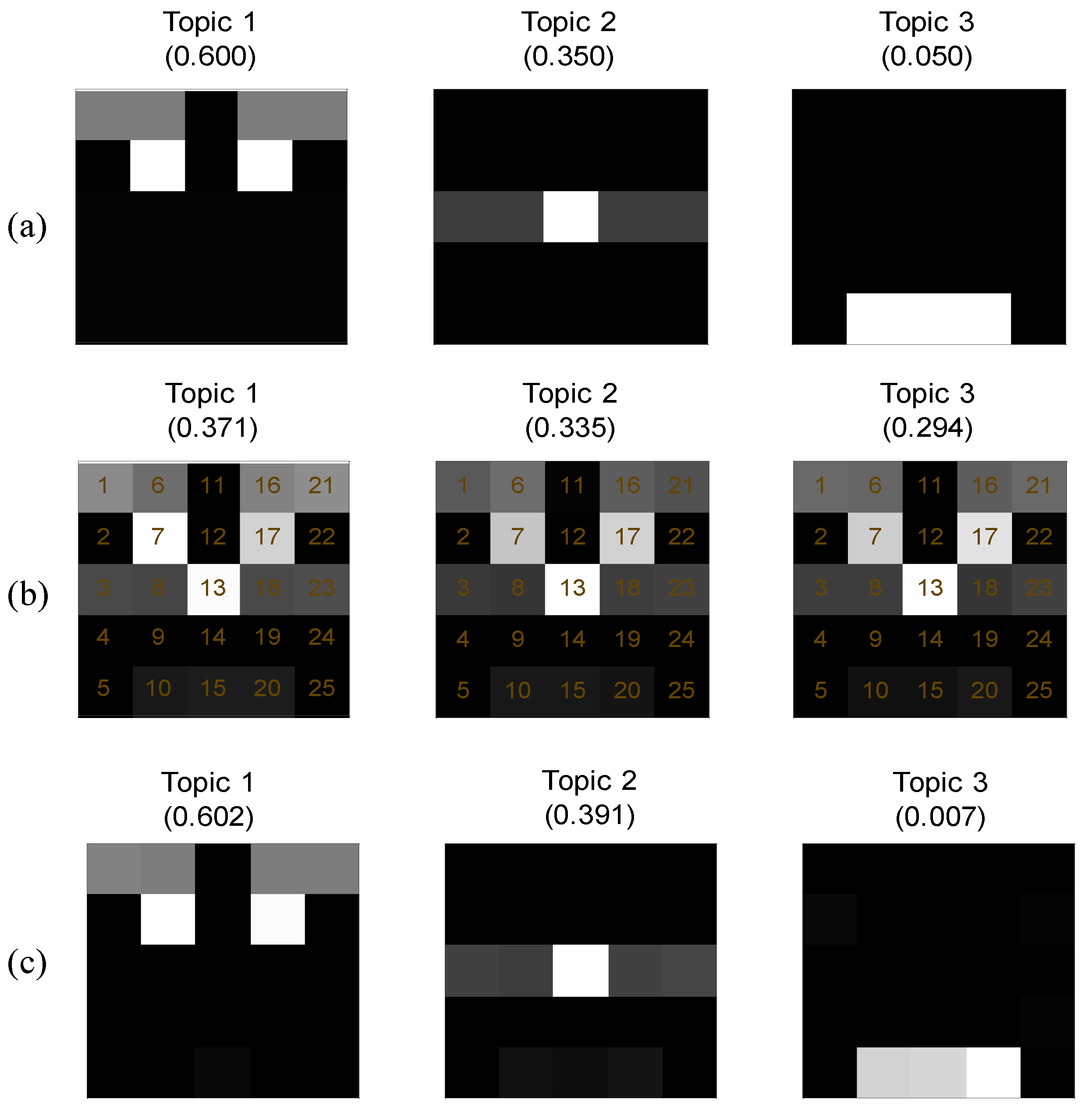
The first five out of 100 total source images each with 100 words for the simple face example are shown in Figure 6. Each word in each document was generated through a random selection among the 3 topics based on the overall topic probabilities: 0.60 for topic 1, 0.35 for topic 2 and 0.05 for topic 3, represented in Figure 7a. This makes the images as 5 × 5 pixels resembling parts of the human face (eyes, nose and mouth).

In the generation process, the pixel index was selected randomly based on the topic probabilities. The document corresponding to the first image is given in Table 1(a). The ordering of the pixel indices within the document is unimportant because of the well-known bag of words assumption common to topic models. Therefore, without loss of generality, we sorted the indices. We then applied 3000 iterations of LDA updating function in Equation (7) with each iteration assigning topics for all the 100 × 100 = 10,000 words. Then, we used the posterior mean formula in Equation (8) to create the initial topic definitions in Figure 7b. Figure 7c is a more accurate representation of the Figure 7a than Figure 7b. This demonstrates the usefulness of the ERT approach intuitively.

In a second stage of the analysis, we prepare the so-called high-level data in Table 1(b) and apply the ERT analysis method to produce the topic definitions in Figure 7c. The high-level data was developed in response to the lack of interpretability of the topics in Figure 7b. As mentioned previously, the high-level data could derive from literal experiments on experts. Here, the subject matter expert (SME) identifies three topics for words in the documents: eyes, nose and mouth. Once the first topic is identified as eyes, the SME uses binomial thought experiments to effectively “erase” all the pixels in topic 1 not relating to eyes. Similarly, for topic 2, all pixels are erased not pertaining to nose. The mouth topic is rare so the SME uses expertise to “draw” the mouth using thought experiments each with two trials and two successes.

Clearly, the ERT model posterior means ϕ values in Figure 7c resemble much more closely the ground truth in Figure 7a than the LDA posterior mean in Figure 7b. One way to quantify topic model accuracy is to use the symmetrized Kullback–Leibler (KL) divergences or “KL distances” from all combinations of estimated topic posterior means to the true topic probabilities [37]. These distances are, formally, $\sum _{x}P\left(x\right)\log \left[\frac{P\left(x\right)}{Q\left(x\right)}\right]+Q\left(x\right)\log \left[\frac{Q\left(x\right)}{P\left(x\right)}\right]$, where $P\left(x\right)$ and $Q\left(x\right)$ are the two distributions (i.e., the case topic models). Being close to the ground truth summarizes both the stability and accuracy of the fit model.

Table 2. Kullback–Leibler (KL) distances from: (a) sampling (S) to LDA topics; (b) sampling to ERT topics.

(a)
True	LDA1	LDA2	LDA3	M.	Distance
True1	5.8401	6.3563	6.0461	1	5.8401
True2	10.4052	9.9058	10.0556	2	9.9058
True3	16.0514	16.0815	16.5708	3	16.5708
(b)
True	ERT1	ERT2	ERT3	M	Distance
True1	0.1480	25.6169	25.6613	1	0.1480
True2	25.9283	1.4619	26.3251	2	1.4619
True3	19.9218	15.5279	0.3864	3	0.3864

(a) shows the KL distances for the LDA posterior mean ϕ and Table 2(b) shows the distances for the ERT model posterior mean ϕ. The closeness is measured by identifying the combination of true and estimated topic pairing that minimize the sum of distances and then comparing the resulting distances. The gain from adding the 25 high-level data points in Table 1(b) is apparent. For example, the maximum distance for the LDA model is 16.5 units while the maximum distance for the ERT model is 1.5 units.

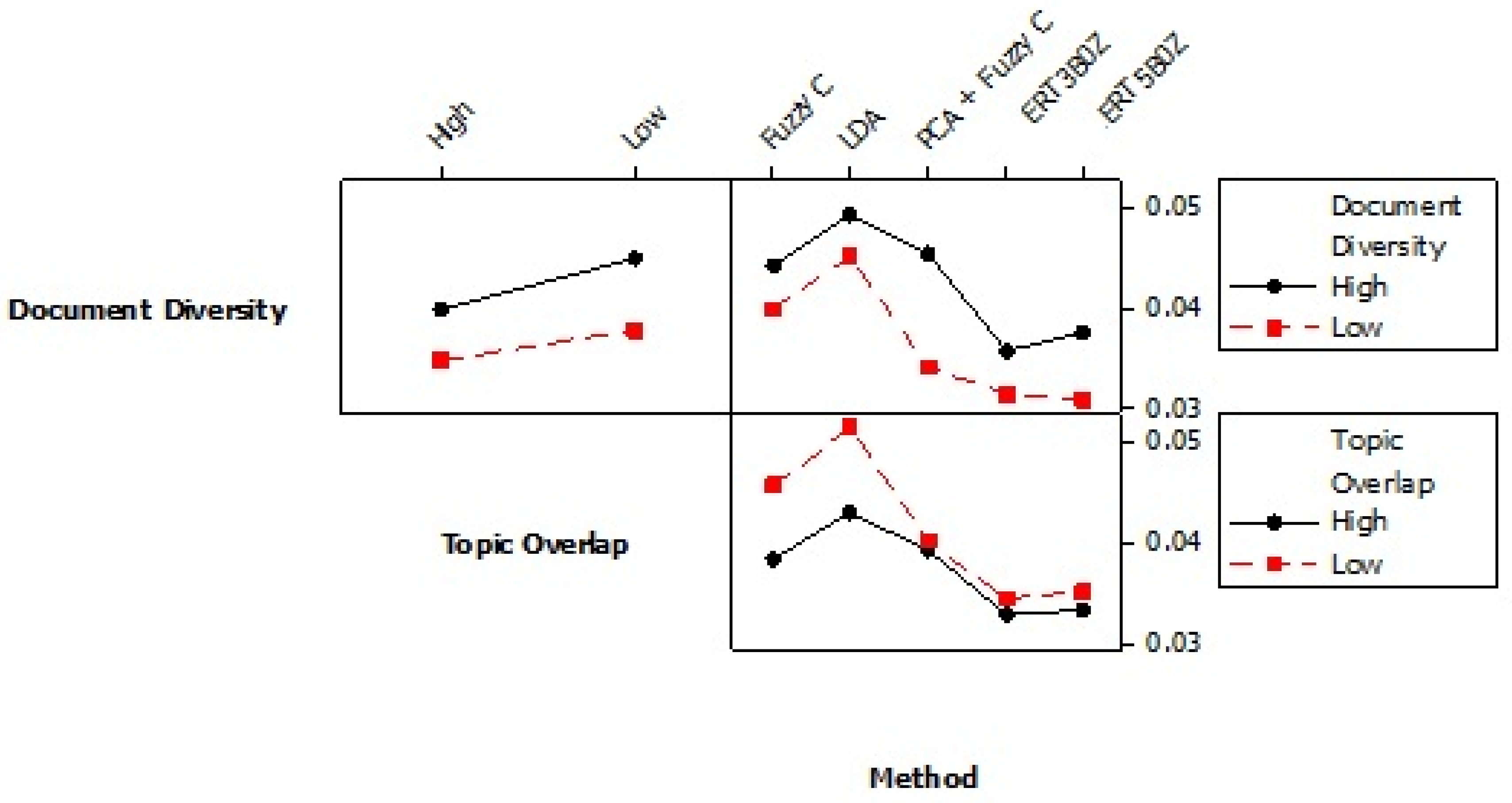
In our previous research relating to text analysis [4], we describe the fuzzy c means clustering methods and pre-processing using principle components analysis (PCA) followed by fuzzy c means clustering. We also defined the minimum average root mean squared (MARMS) error. This is the difference between the estimated topic definitions probabilities and the ground truth values from the simulation root mean squared. Here, we include part of the results of the computational experiment omitted from 4 for space reasons. Figure 8 shows the accuracies of the various alternatives including two ERT variations. The first ERT variation has three high level data points per topic. The second has five per topic.

Note that there is replication error from the simulation such that only a portion of the factor effects was found to be significant. For example, the different between the ERT variations is not significant but the improvement over the alternatives is significant. The comparison shows that ERT offers reduced errors regardless of document how diverse or different the simulated documents are (document diversity) and how much overlap the topics have in using the same words or pixels (topic overlap).

5.2. Bar Example

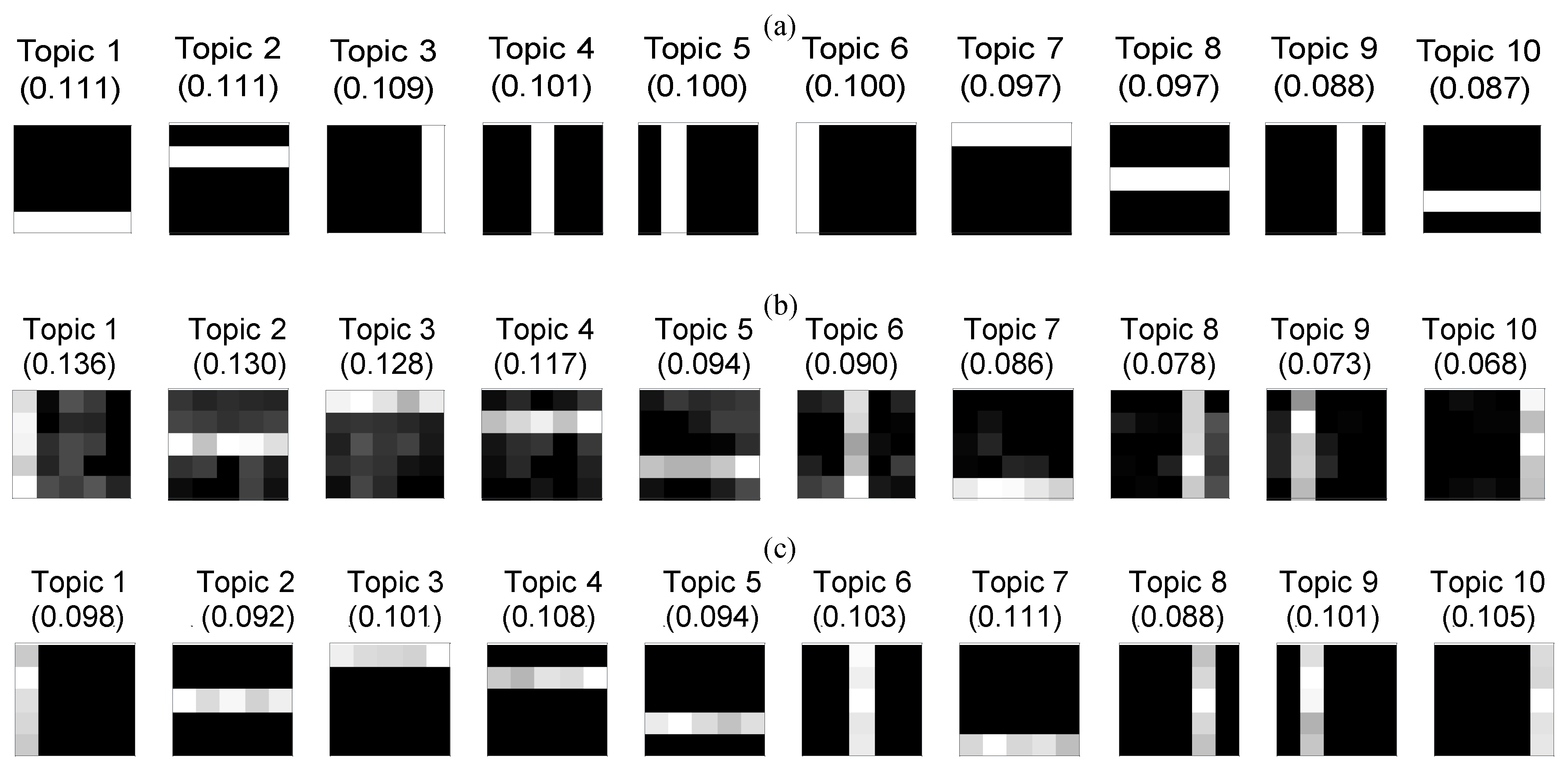
Figure 9a shows the ground truth model for a 10-topic example involving vertical and horizontal bars from [35]. In the original example, the authors sampled 1000 documents each of length 100 words and the derived LDA model based on Equations (7) and (8) very closely resembled the true model. Our purpose is to evaluate a more challenging case with only D = 200 document with N_d = 100-pixel indices (words). Each of the 20,000 low-level words is derived from first sampling the topic with the topic probabilities given in Figure 9a and then sampling the words based on the probabilities indicated in the images. The derived LDA posterior mean values from 3000 collapsed Gibbs sampling iterations are pictured in Figure 9b. Without loss of generality, we order the estimated topics by their posterior mean topic proportions, shown in parentheses in Figure 9b.

In general, the estimated posterior means in Figure 9b are identifiable as either vertical or horizontal bars. Therefore, the function of the second stage editing using the high-level data in

Table 3. The 200 high-level data points for the bar numerical example. This shows many zaps in the topic definitions.

#	t	c	N	x	#	t	c	N	x	#	t	c	N	x	#	t	c	N	x
1	1	6	1M	0	51	3	14	1M	0	101	6	1	1M	0	151	8	11	1M	0
2	1	7	1M	0	52	3	15	1M	0	102	6	2	1M	0	152	8	12	1M	0
3	1	8	1M	0	53	3	17	1M	0	103	6	3	1M	0	153	8	13	1M	0
4	1	9	1M	0	54	3	18	1M	0	104	6	4	1M	0	154	8	14	1M	0
5	1	10	1M	0	55	3	19	1M	0	105	6	5	1M	0	155	8	15	1M	0
6	1	11	1M	0	56	3	20	1M	0	106	6	6	1M	0	156	8	21	1M	0
7	1	12	1M	0	57	3	22	1M	0	107	6	7	1M	0	157	8	22	1M	0
8	1	13	1M	0	58	3	23	1M	0	108	6	8	1M	0	158	8	23	1M	0
9	1	14	1M	0	59	3	24	1M	0	109	6	9	1M	0	159	8	24	1M	0
10	1	15	1M	0	60	3	25	1M	0	110	6	10	1M	0	160	8	25	1M	0
11	1	16	1M	0	61	4	1	1M	0	111	6	16	1M	0	161	9	1	1M	0
12	1	17	1M	0	62	4	3	1M	0	112	6	17	1M	0	162	9	2	1M	0
13	1	18	1M	0	63	4	4	1M	0	113	6	18	1M	0	163	9	3	1M	0
14	1	19	1M	0	64	4	5	1M	0	114	6	19	1M	0	164	9	4	1M	0
15	1	20	1M	0	65	4	6	1M	0	115	6	20	1M	0	165	9	5	1M	0
16	1	21	1M	0	66	4	8	1M	0	116	6	21	1M	0	166	9	11	1M	0
17	1	22	1M	0	67	4	9	1M	0	117	6	22	1M	0	167	9	12	1M	0
18	1	23	1M	0	68	4	10	1M	0	118	6	23	1M	0	168	9	13	1M	0
19	1	24	1M	0	69	4	11	1M	0	119	6	24	1M	0	169	9	14	1M	0
20	1	25	1M	0	70	4	13	1M	0	120	6	25	1M	0	170	9	15	1M	0
21	2	1	1M	0	71	4	14	1M	0	121	7	1	1M	0	171	9	16	1M	0
22	2	2	1M	0	72	4	15	1M	0	122	7	2	1M	0	172	9	17	1M	0
23	2	4	1M	0	73	4	16	1M	0	123	7	3	1M	0	173	9	18	1M	0
24	2	5	1M	0	74	4	18	1M	0	124	7	4	1M	0	174	9	19	1M	0
25	2	6	1M	0	75	4	19	1M	0	125	7	6	1M	0	175	9	20	1M	0
26	2	7	1M	0	76	4	20	1M	0	126	7	7	1M	0	176	9	21	1M	0
27	2	9	1M	0	77	4	21	1M	0	127	7	8	1M	0	177	9	22	1M	0
28	2	10	1M	0	78	4	23	1M	0	128	7	9	1M	0	178	9	23	1M	0
29	2	11	1M	0	79	4	24	1M	0	129	7	11	1M	0	179	9	24	1M	0
30	2	12	1M	0	80	4	25	1M	0	130	7	12	1M	0	180	9	25	1M	0
31	2	14	1M	0	81	5	1	1M	0	131	7	13	1M	0	181	10	1	1M	0
32	2	15	1M	0	82	5	2	1M	0	132	7	14	1M	0	182	10	2	1M	0
33	2	16	1M	0	83	5	3	1M	0	133	7	16	1M	0	183	10	3	1M	0
34	2	17	1M	0	84	5	5	1M	0	134	7	17	1M	0	184	10	4	1M	0
35	2	19	1M	0	85	5	6	1M	0	135	7	18	1M	0	185	10	5	1M	0
36	2	20	1M	0	86	5	7	1M	0	136	7	19	1M	0	186	10	6	1M	0
37	2	21	1M	0	87	5	8	1M	0	137	7	21	1M	0	187	10	7	1M	0
38	2	22	1M	0	88	5	10	1M	0	138	7	22	1M	0	188	10	8	1M	0
39	2	24	1M	0	89	5	11	1M	0	139	7	23	1M	0	189	10	9	1M	0
40	2	25	1M	0	90	5	12	1M	0	140	7	24	1M	0	190	10	10	1M	0
41	3	2	1M	0	91	5	13	1M	0	141	8	1	1M	0	191	10	11	1M	0
42	3	3	1M	0	92	5	15	1M	0	142	8	2	1M	0	192	10	12	1M	0
43	3	4	1M	0	93	5	16	1M	0	143	8	3	1M	0	193	10	13	1M	0
44	3	5	1M	0	94	5	17	1M	0	144	8	4	1M	0	194	10	14	1M	0
45	3	7	1M	0	95	5	18	1M	0	145	8	5	1M	0	195	10	15	1M	0
46	3	8	1M	0	96	5	20	1M	0	146	8	6	1M	0	196	10	16	1M	0
47	3	9	1M	0	97	5	21	1M	0	147	8	7	1M	0	197	10	17	1M	0
48	3	10	1M	0	98	5	22	1M	0	148	8	8	1M	0	198	10	18	1M	0
49	3	12	1M	0	99	5	23	1M	0	149	8	9	1M	0	199	10	19	1M	0
50	3	13	1M	0	100	5	25	1M	0	150	8	10	1M	0	200	10	20	1M	0

is to clean up or erase the blemishes to the topic definitions. By saying that in one out of 1M binomial thought experiments, zero would have a specific word on a topic, that word is erased or zapped from the definition. Similarly, other words could be boosted but Table 3 only contains zaps. Figure 9c shows the posterior means derived from 3000 iterations of collapsed Gibbs ERT model sampling using the approximate updating and mean estimation formulas in Equations (11)–(14).

With 10 topics, there is greater ambiguity about how the estimated topics map onto the ground truth topics.

Table 4. KL distances from: (a) sampling (S) to LDA topics; (b) sampling to ERT (SM) topics.

(a)
True	LDA1	LDA2	LDA3	LDA4	LDA5	LDA6	LDA7	LDA8	LDA9	LDA10	M.	SKLD
True1	11.735	17.543	17.072	18.732	16.917	11.487	1.625	15.089	17.305	14.733	7	1.625
True2	15.367	13.628	14.362	4.175	15.719	16.352	20.028	13.045	13.831	15.554	4	4.175
True3	19.184	13.224	14.740	11.620	10.874	16.358	16.846	13.438	20.525	0.826	10	0.826
True4	13.354	15.048	12.553	14.818	15.444	4.040	15.638	18.329	17.717	18.037	6	4.040
True5	15.957	14.095	11.527	13.543	15.472	17.619	13.433	18.227	2.181	18.782	9	2.181
True6	5.810	12.624	12.989	15.081	15.195	16.413	15.618	18.551	16.902	20.962	1	5.810
True7	14.073	14.527	5.976	16.036	13.825	12.995	20.513	16.851	17.520	14.544	3	5.976
True8	12.944	5.982	14.020	15.453	18.161	17.094	18.289	14.326	14.613	15.857	2	5.982
True9	15.137	12.078	14.484	16.773	12.799	18.294	15.991	3.767	19.836	18.757	8	3.767
True10	15.323	15.389	14.863	17.439	5.164	14.795	17.071	13.000	13.891	16.676	5	5.164
(b)
True	SM1	SMS2	SM3	SM4	SM5	SM6	SM7	SM8	SM9	SM10	M.	SKLD
True1	20.984	25.917	25.917	25.920	25.918	20.823	0.006	21.026	21.052	20.731	7	0.006
True2	20.198	25.917	25.917	0.009	25.918	20.775	25.919	20.776	20.219	20.947	4	0.009
True3	25.918	20.668	20.324	20.161	20.768	25.916	21.174	25.919	25.922	0.003	10	0.003
True4	25.918	20.571	20.924	20.577	20.845	0.001	20.817	25.919	25.922	25.917	6	0.001
True5	25.918	20.931	20.875	21.237	20.296	25.916	20.230	25.919	0.013	25.917	9	0.013
True6	0.005	20.422	20.595	20.989	20.604	25.916	20.817	25.919	25.922	25.917	1	0.005
True7	20.968	25.917	0.004	25.920	25.918	20.610	25.919	21.026	20.707	20.862	3	0.004
True8	20.710	0.004	25.917	25.920	25.918	20.548	25.919	20.124	20.354	20.354	2	0.004
True9	25.918	21.081	20.956	20.726	21.165	25.916	20.643	0.007	25.922	25.917	8	0.007
True10	20.818	25.917	25.917	25.920	0.006	20.909	25.919	20.730	21.368	20.777	5	0.006

(a) shows the KL distances from the true topics to the estimated topics derived using LDA. Table 4(b) shows the KL distances from the true topics to the estimated topics using ERT posterior mean probabilities. The largest distance is reduced from 6.0 units to 0.013 units through the addition of the 25 high-level data points and the application of the ERT model.

5.3. Fashion Example

Next, we consider the “Fashion-MNIST” dataset with 10,000 28 × 28-pixel grayscale images [43]. The dataset is tagged with 10 categories: t-shirt/top, trouser, pullover, dress, coat, sandal, shirt, sneaker, bag and ankle boot. In a preprocessing step, we reduce the number of grayscale levels by a factor of 200 to keep our document lengths sufficiently small for our VBA implementation storage sizes. The granularity seems visually acceptable for differentiating between categories (Figure 10a–c). Next, we created the documents by repeating the pixel numbers proportionally to the reduced gray scale values. For example, a value of 2 for pixel 37 results in “37, 37” being included in the document.

With all 10,000 images and 10 topics, LDA can approximately recover the categories as shown in Figure 10a. This figure is based on 500 iterations. Note that the skinny dress is apparently missing and there are two tea shirts. When analyzed using LDA and only the first 1000 images and again 500 iterations, the results are blurrier, and the dress is still missing as shown in Figure 10b. If the top 20 pixels for the LDA run are used to supervise the ERT model based on 1000 datapoints, the result from 300 iterations is shown in Figure 10c. This required approximately 11 h using an i7 1.8 GHz processor with 16 GB of RAM. The result is arguably more accurate than LDA based on all 10,000 images because the dress appears as topic 6 and there is only a single tea shirt.

5.4. Tungsten Inert Gas Welding Example

Next, we consider the “Tungsten Inert Gas (TIG) Welding” dataset with 10,000 20 × 20 truncated pixel grayscale images [44]. The dataset is tagged with 6 categories: good weld, burn through, contamination, lack of fusion, misalignment and lack of penetration. In a preprocessing step, we reduce the number of grayscale levels by a factor of 50 to keep our document lengths sufficiently small for our VBA implementation storage sizes. The granularity seems visually acceptable for differentiating between categories (Figure 10d–f). Next, we created the documents by repeating the pixel numbers proportionally to the reduced gray scale values.

With all 10,000 images and 10 topics, LDA can approximately recover the categories as shown in Figure 10d. This figure is based on 500 iterations. Note that all the topics are difficult for us to interpret with the naked eye (as is true for the images with a few exceptions). When analyzed using LDA and only the first 1000 images and again 500 iterations, the results are blurrier (Figure 10e). If the top 20 pixels for the LDA run are used to supervise the ERT model based on 1000 datapoints, the result from 50 iterations is shown in Figure 10f. This required approximately 1 h using an i7 1.8 GHz processor with 16 GB of RAM. The result is arguably more like the ideal pictures in [45] accurate than either LDA application.

6. Results: Laser Welding Study

In the previous section, we applied ERT modeling to two numerical examples in which the ground truth was known. Next, we focus on analyzing the 20 source images for the laser welding aluminum alloy study shown in Figure 1. None of the LDA derived posterior mean topics in Figure 2 directly corresponded to any of the nonconformity issues in Figure 3 from standard textbooks [30]. As a result, even if we could perfectly classify the existing or new welds perfectly into the LDA derived topics, we would have difficulty documenting the failures and analyzing their causes.

Looking at the source welds, we can clearly identify which welds have which nonconformities as pictured in Figure 3. Therefore, we have “expert” judgment that the classical nonconformity codes are relevant. We began our development of the 198 high-level data in

Table 5. The 198 high-level data points for the laser welding example.

#	t	c	N	x	#	t	c	N	x	#	t	c	N	x	#	t	c	N	x
1	1	58	20	20	51	2	106	20	20	101	3	148	20	20	151	4	111	20	20
2	1	59	20	20	52	2	107	20	20	102	3	149	20	20	152	4	131	20	20
3	1	66	10	10	53	2	108	20	20	103	3	154	20	20	153	4	185	20	20
4	1	67	10	10	54	2	109	20	20	104	3	156	20	20	154	4	169	20	20
5	1	68	10	10	55	2	110	20	20	105	3	165	20	20	155	4	171	20	20
6	1	69	10	10	56	2	126	20	20	106	3	166	20	20	156	4	177	20	20
7	1	70	10	10	57	2	127	20	20	107	3	167	20	20	157	4	178	20	20
8	1	71	10	10	58	2	128	20	20	108	3	168	20	20	158	4	186	20	20
9	1	72	10	10	59	2	129	20	20	109	3	170	20	20	159	4	187	20	20
10	1	73	20	20	60	2	130	20	20	110	3	174	20	20	160	4	188	20	20
11	1	74	20	20	61	2	131	20	20	111	3	175	20	20	161	5	64	20	20
12	1	75	20	20	62	2	59	20	20	112	3	176	20	20	162	5	65	20	20
13	1	76	20	20	63	2	77	20	20	113	3	190	20	20	163	5	66	20	20
14	1	77	20	20	64	2	78	20	20	114	3	192	20	20	164	5	69	20	20
15	1	78	20	20	65	2	79	20	20	115	4	44	1M	0	165	5	84	20	20
16	1	79	20	20	66	2	96	20	20	116	4	84	10	10	166	5	85	20	20
17	1	87	10	10	67	2	97	20	20	117	4	104	10	10	167	5	86	20	20
18	1	88	10	10	68	2	98	20	20	118	4	5	20	20	168	5	87	20	20
19	1	89	10	10	69	2	99	20	20	119	4	11	20	20	169	5	88	20	20
20	1	90	10	10	70	2	116	20	20	120	4	14	20	20	170	5	89	20	20
21	1	91	10	10	71	2	117	20	20	121	4	15	20	20	171	5	90	20	20
22	1	92	20	20	72	2	118	20	20	122	4	16	20	20	172	5	92	20	20
23	1	93	20	20	73	2	119	20	20	123	4	17	20	20	173	5	93	20	20
24	1	94	20	20	74	2	137	20	20	124	4	18	20	20	174	5	104	20	20
25	1	95	20	20	75	2	138	20	20	125	4	30	20	20	175	5	105	20	20
26	1	96	20	20	76	2	139	20	20	126	4	32	20	20	176	5	106	20	20
27	1	97	20	20	77	2	43	1M	0	127	4	33	20	20	177	5	107	20	20
28	1	98	20	20	78	2	81	1M	0	128	4	35	20	20	178	5	108	20	20
29	1	99	20	20	79	3	83	1M	0	129	4	36	20	20	179	5	109	20	20
30	1	199	30	30	80	3	103	1M	0	130	4	37	20	20	180	5	110	20	20
31	1	22	1M	0	81	3	6	20	20	131	4	38	20	20	181	5	111	20	20
32	1	162	1M	0	82	3	10	20	20	132	4	50	20	20	182	5	112	20	20
33	1	185	10	10	83	3	12	20	20	133	4	48	20	20	183	5	113	20	20
34	2	46	10	10	84	3	13	20	20	134	4	53	20	20	184	5	114	20	20
35	2	148	20	20	85	3	34	20	20	135	4	54	20	20	185	5	124	20	20
36	2	46	20	20	86	3	26	20	20	136	4	56	20	20	186	5	125	20	20
37	2	47	20	20	87	3	45	20	20	137	4	65	20	20	187	5	126	20	20
38	2	48	20	20	88	3	46	20	20	138	4	66	20	20	188	5	127	20	20
39	2	49	20	20	89	3	47	20	20	139	4	69	20	20	189	5	128	20	20
40	2	50	20	20	90	3	49	20	20	140	4	71	20	20	190	5	129	20	20
41	2	66	20	20	91	3	59	20	20	141	4	72	20	20	191	5	130	20	20
42	2	67	20	20	92	3	125	20	20	142	4	73	20	20	192	5	131	20	20
43	2	68	20	20	93	3	126	20	20	143	4	74	20	20	193	5	132	20	20
44	2	69	20	20	94	3	127	20	20	144	4	75	20	20	194	5	133	20	20
45	2	70	20	20	95	3	128	20	20	145	4	76	20	20	195	5	134	20	20
46	2	86	20	20	96	3	129	20	20	146	4	77	20	20	196	5	135	20	20
47	2	87	20	20	97	3	130	20	20	147	4	78	20	20	197	5	158	20	20
48	2	88	20	20	98	3	145	20	20	148	4	86	20	20	198	5	159	20	20
49	2	89	20	20	99	3	146	20	20	149	4	87	20	20
50	2	90	20	20	100	3	147	20	20	150	4	105	20	20

, by identifying an approximate correspondence between the topics in Figure 2 and the ideals in Figure 3. We identified topic 1 as undercut, topic 2 as stickout, topic 3 as good welds, topic 4 as backside undercut and topic 5 as stickout and undercut. Intuitively, we boosted parts of the images that look like the architypes in Figure 3 and zapped the other parts.

With these identifications, we then determined which pixels needed erasing and which pixels needed boosting or addition. We did this manually but with software there is the possibility of selecting the pixels en-mass in a fully interactive fashion. Most of the topics had large sections of pixels that needed filling-in but a few pixels required erasure. For example, all the pixels in the lower middle section of topic 1 needed boosting so that the resulting topic definition in Figure 11 resembled undercut in Figure 3.

Once we identified the high-level data set, our custom C++ software was able to perform 3000 iterations of collapsed Gibbs sampling and derive the posterior mean probabilities shown in Figure 11 in 12 min on our 2.5 GHz Core 2 Quad processor.

Results from four alternative cluster definition methods are described in Figure 11. The fuzzy c method only identifies topics 1 and 2 accurately in terms of standard conventions in Figure 3. LDA is only marginally better in Figure 11b. Principal Component Analysis (PCA) followed by fuzzy identifies approximately three topics correctly.

For ERT, examination of the posterior mean probabilities for the document-topic probabilities, ${\theta }_d$, provides both an indication of the value of the derived ERT model and a level of validation.

Table 6. Topic assignment probabilities from the ERT for the 20 laser welding images.

	1st Topic (Prob.)	2nd Topic (Prob.)	3rd Topic (Prob.)	4th Topic (Prob.)	5th Topic (Prob.)
source 1	5 (0.675)	2 (0.316)	1 (0.005)	3 (0.004)	4 (0.000)
source 2	5 (0.904)	4 (0.093)	1 (0.002)	2 (0.001)	3 (0.000)
source 3	3 (0.896)	5 (0.091)	4 (0.012)	2 (0.001)	1 (0.000)
source 4	3 (0.749)	5 (0.162)	4 (0.088)	1 (0.000)	2 (0.000)
source 5	3 (0.648)	2 (0.166)	5 (0.106)	4 (0.080)	1 (0.000)
source 6	3 (0.689)	5 (0.220)	4 (0.089)	1 (0.002)	2 (0.000)
source 7	5 (0.826)	2 (0.165)	4 (0.006)	1 (0.002)	3 (0.001)
source 8	5 (0.747)	2 (0.252)	1 (0.001)	3 (0.000)	4 (0.000)
source 9	3 (0.898)	2 (0.057)	5 (0.040)	4 (0.002)	1 (0.002)
source 10	3 (0.951)	4 (0.042)	5 (0.008)	1 (0.000)	2 (0.000)
source 11	3 (0.685)	5 (0.210)	4 (0.101)	1 (0.004)	2 (0.000)
source 12	3 (0.748)	2 (0.225)	4 (0.014)	1 (0.011)	5 (0.003)
source 13	4 (0.583)	2 (0.406)	3 (0.006)	5 (0.005)	1 (0.000)
source 14	2 (0.735)	4 (0.258)	1 (0.005)	3 (0.001)	5 (0.001)
source 15	2 (0.714)	4 (0.278)	1 (0.006)	5 (0.001)	3 (0.001)
source 16	3 (0.986)	4 (0.008)	5 (0.003)	1 (0.002)	2 (0.001)
source 17	4 (0.803)	2 (0.197)	3 (0.000)	1 (0.000)	5 (0.000)
source 18	1 (0.780)	5 (0.214)	3 (0.004)	2 (0.002)	4 (0.000)
source 19	1 (0.994)	4 (0.003)	3 (0.002)	5 (0.001)	2 (0.000)
source 20	1 (0.521)	4 (0.478)	3 (0.001)	2 (0.000)	5 (0.000)

shows the document-topic probabilities based on the topic definitions in Figure 11d. If we interpret these probabilities as indications of the probability each topic is relevant, we find that the most probable topics match in 20 out of 20 cases how a subject matter expert (SME) would classify the source welds. For example, the first image (source 1) clearly corresponds to a weld with both undercut and stickout. Clearly, engineers would find these probabilities significantly more relevant than probabilities for LDA model topic in Figure 2.

7. Discussion

The authors have significant experience applying topic models to real-world data sets. In our applications, we have often found that the initially derived topic model definitions usually were more interpretable than the LDA topics for the welding and simple face problems (Figure 2 and Figure 7b) but less comprehensible than the LDA topics for the bar example in Figure 8b. So far, we have never encountered an example in which we did not wish that we could edit some or all of the topics to enhance the model accuracy and/or subjective interpretability.

The intent of the proposed subject matter expert refined topic (ERT) models with their handles is to facilitate user interaction with the models, i.e., the directability. We suggest that model handles function in relation to topic models in an analogous manner erasers function in relation to pencils. Admittedly, there is a need to balance between the degree of subjectivity possibly entering through the handle and the relative objectivity of the ordinary low-level data. In our primary application, we included supervision of only 198 out of 200 × 5 = 1000 possible pixels or 19.8%. With this limited addition, we have derived highly interpretable topic definitions in the form of posterior mean ϕ. In addition, we have achieved perfect assignment of the source welds to the interpretable topic definitions or clusters (20/20).

There are important limitations of current codes. First, the number of grayscale levels must be reduced (generally) to achieve manageable file sizes. This issue is not special to ERT and relates to the bag of words image representation in which each grayscale level makes the documents proportionally longer. Reducing granularity can make the images blurry, e.g., see Figure 9. In addition, in ERT the user must boost almost every topic, or the estimation will adjust such that the zapping will apply harmlessly to images with darkness already at the associated pixel locations. Yet, the effort to boost each topic can be minimal. For example, we supplied only 20 pixels (out of 784 pixels) per topic to supervise the Fashion MNIST images in Section 5.

8. Conclusions

In conclusion, in this article we propose a method to edit the cluster definitions in topic modeling with applications in image analysis. The proposed method creates high-level data which is a potentially important concept with a broad range of possible applications. We demonstrate in our numerical example that the proposed ERT modeling method can derive more accurate and more stable topic model fits than LDA. In addition, for our main laser welding application we show that a small amount of high-level data is able to perturb the model so that the clusters align with intuitive and popular definitions of defects or nonconformities. We suggest that the concepts of ERT and handles can be explored in a wide range of supervised and unsupervised modeling situations. The resulting high-level data may become a major output from knowledge workers in the future.

There are a number of opportunities for future work. First, more computationally efficient and stable methods for fitting ERT models to images can be developed. The collapsed Gibbs sampling method is only approximate for cases with more than a single zap and it can be time consuming. Second, other types of high-level data besides boosts and zaps can be developed. Perhaps these might relate to archetypal images. Third, the concept of handles can be extended to other types of distribution fits such as regression and time series modeling. Fourth, more efficient methods for image processing besides the bag of words methods can be explored and related to ERT-type modeling. The document lengths can be prohibitively long if too many gray scale gradations are applied in the current representations. New representations can be studied that are more concise. Fifth, documented editing using ERT can be enhanced with tablet applications that permit quick boosting (using pen-type features) and zapping (using eraser-type features). Fifth, exploration of the E-M algorithm for ERT procedures could speed up estimation. Using standard notation [13], we have ${\varphi }_{d,t,c}$ as the document-specific estimated topic definition probabilities, ${\varphi }_{d,t,c}$, and the document-specific indicator function for the words is $w_{d,n}^c$. We conjecture that the conditional multinomial may approximately satisfy:

$${\varphi }_{t,c}\propto \{\begin{array}{c}0 if {\mathrm{N}}_{t,c}\gg 0; {\mathrm{x}}_{t,c}=0 \left(zaps\right)\\ {\displaystyle {\displaystyle \sum }_{d=1}^D}{\displaystyle {\displaystyle \sum }_{n=1}^{N_d}}\left({\varphi }_{d,t,c}+\frac{x_{t,c}}{N_d+N_{t,c}}\right)w_{d,n}^{c}otherwise \left(boosts\right)\end{array}$$

(15)

Further, accuracy issues associated with ERT models can be studied further including through investigating alternatives quality measures (to KL distance) such as topic model semantic [46] and topic [47] coherence measures.

References

- Reese, C.S.; Wilson, A.G.; Guo, J.; Hamada, M.S.; Johnson, V.E. A Bayesian model for integrating multiple sources of lifetime information in system-reliability assessments. J. Qual. Technol. 2011, 43, 127–141. [Google Scholar] [CrossRef]
- Nair, V. Special Issue on Statistics in Information Technology. Technometrics 2007, 49, 236. [Google Scholar] [CrossRef]
- Nembhard, H.B.; Ferrier, N.J.; Osswald, T.A.; Sanz-Uribe, J.R. An integrated model for statistical and vision monitoring in manufacturing transitions. Qual. Reliab. Eng. Int. 2003, 19, 461–476. [Google Scholar] [CrossRef]
- Allen, T.T.; Xiong, H.; Afful-Dadzie, A. A directed topic model applied to call center improvement. Appl. Stoch. Models Bus. Ind. 2016, 32, 57–73. [Google Scholar] [CrossRef]
- Allen, T.T.; Sui, Z.; Parker, N.L. Timely decision analysis enabled by efficient social media modeling. Decis. Anal. 2017, 14, 250–260. [Google Scholar] [CrossRef]
- Megahed, F.M.; Woodall, W.H.; Camelio, J.A. A review and perspective on control charting with image data. J. Qual. Technol. 2011, 43, 83–98. [Google Scholar] [CrossRef]
- Colosimo, B.M.; Pacella, M. Analyzing the effect of process parameters on the shape of 3D profiles. J. Qual. Technol. 2011, 43, 169–195. [Google Scholar] [CrossRef]
- Hansen, M.H.; Nair, V.N.; Friedman, D.J. Monitoring wafer map data from integrated circuit fabrication processes for spatially clustered defects. Technometrics 1997, 39, 241–253. [Google Scholar] [CrossRef]
- Huang, D.; Allen, T.T. Design and analysis of variable fidelity experimentation applied to engine valve heat treatment process design. J. R. Stat. Soc. Ser. C (Appl. Stat.) 2005, 54, 443–463. [Google Scholar] [CrossRef]
- Ferreiro, S.; Sierra, B.; Irigoien, I.; Gorritxategi, E. Data mining for quality control: Burr detection in the drilling process. Comput. Ind. Eng. 2011, 60, 801–810. [Google Scholar] [CrossRef]
- Alfaro-Almagro, F.; Jenkinson, M.; Bangerter, N.K.; Andersson, J.L.; Griffanti, L.; Douaud, G.; Sotiropoulos, S.N.; Jbabdi, S.; Hernandez-Fernandez, M.; Vallee, E. Image processing and Quality Control for the first 10,000 brain imaging datasets from UK Biobank. Neuroimage 2018, 166, 400–424. [Google Scholar] [CrossRef] [PubMed]
- Apley, D.W.; Lee, H.Y. Simultaneous identification of premodeled and unmodeled variation patterns. J. Qual. Technol. 2010, 42, 36–51. [Google Scholar] [CrossRef]
- Blei, D.M.; Ng, A.Y.; Jordan, M.I. Latent Dirichlet Allocation. J. Mach. Learn. Res. 2003, 3, 993–1022. [Google Scholar]
- Murray, J.S.; Reiter, J.P. Multiple imputation of missing categorical and continuous values via Bayesian mixture models with local dependence. J. Am. Stat. Assoc. 2016, 111, 1466–1479. [Google Scholar] [CrossRef] [Green Version]
- Miller, J.W.; Harrison, M.T. Mixture models with a prior on the number of components. J. Am. Stat. Assoc. 2018, 113, 340–356. [Google Scholar] [CrossRef]
- Van Havre, Z.; White, N.; Rousseau, J.; Mengersen, K. Overfitting Bayesian mixture models with an unknown number of components. PLoS ONE 2015, 10, e0131739. [Google Scholar] [CrossRef] [PubMed] [Green Version]
- Ma, Z.; Lai, Y.; Kleijn, W.B.; Song, Y.-Z.; Wang, L.; Guo, J. Variational Bayesian learning for Dirichlet process mixture of inverted Dirichlet distributions in non-Gaussian image feature modeling. IEEE Trans. Neural Netw. Learn. Syst. 2018, 30, 449–463. [Google Scholar] [CrossRef]
- Tseng, S.H.; Allen, T. A Simple Approach for Multi-fidelity Experimentation Applied to Financial Engineering. Appl. Stoch. Models Bus. Ind. 2015, 31, 690–705. [Google Scholar] [CrossRef]
- Jeske, D.R.; Liu, R.Y. Mining and tracking massive text data: Classification, construction of tracking statistics, and inference under misclassification. Technometrics 2007, 49, 116–128. [Google Scholar] [CrossRef]
- Genkin, A.; Lewis, D.D.; Madigan, D. Large-scale Bayesian logistic regression for text categorization. Technometrics 2007, 49, 291–304. [Google Scholar] [CrossRef] [Green Version]
- Topalidou, E.; Psarakis, S. Review of multinomial and multiattribute quality control charts. Qual. Reliab. Eng. Int. 2009, 25, 773–804. [Google Scholar] [CrossRef]
- Blei, D.M.; Lafferty, J.D. A correlated topic model of science. Ann. Appl. Stat. 2007, 1, 17–35. [Google Scholar] [CrossRef] [Green Version]
- Blei, D.M.; Mcauliffe, J.D. Supervised topic models. In Proceedings of the 20th International Conference on Neural Information Processing Systems, Vancouver, BC, Canada, 3–6 December 2007; pp. 121–128. [Google Scholar]
- Dunn, J.C. A fuzzy relative of the ISODATA process and its use in detecting compact well-separated Clust. J. Cybern. 1973, 3, 32–57. [Google Scholar] [CrossRef]
- Liao, T.; Li, D.-M.; Li, Y.-M. Detection of welding flaws from radiographic images with fuzzy clustering methods. Fuzzy Sets Syst. 1999, 108, 145–158. [Google Scholar] [CrossRef]
- Sebzalli, Y.; Wang, X. Knowledge discovery from process operational data using PCA and fuzzy clustering. Eng. Appl. Artif. Intell. 2001, 14, 607–616. [Google Scholar] [CrossRef]
- Yan, H.; Paynabar, K.; Shi, J. Image-based process monitoring using low-rank tensor decomposition. IEEE Trans. Autom. Sci. Eng. 2014, 12, 216–227. [Google Scholar] [CrossRef]
- Qiu, P. Jump regression, image processing, and quality control. Qual. Eng. 2018, 30, 137–153. [Google Scholar] [CrossRef]
- Rosen-Zvi, M.; Chemudugunta, C.; Griffiths, T.; Smyth, P.; Steyvers, M. Learning author-topic models from text corpora. ACM Trans. Inf. Syst. (TOIS) 2010, 28, 1–38. [Google Scholar] [CrossRef]
- Ihianle, I.K.; Naeem, U.; Islam, S.; Tawil, A.-R. A Hybrid Approach to Recognising Activities of Daily Living from Object Use in the Home Environment. Informatics 2018, 5, 6. [Google Scholar] [CrossRef] [Green Version]
- Arun, R.; Suresh, V.; Madhavan, V.C.E.; Murty, N.M. On Finding the Natural Number of Topics with Latent Dirichlet Allocation: Some Observations. In Pacific-Asia Conference on Knowledge Discovery and Data Mining; Springer: Berlin/Heidelberg, Germany, 2010; pp. 391–402. [Google Scholar]
- Jeffus, L.; Bower, L. Welding Skills, Processes and Practices for Entry-Level Welders; Cengage Learning: Boston, MA, USA, 2009. [Google Scholar]
- Cao, J.; Xia, T.; Li, J.; Zhang, Y.; Tang, S. A Density-Based Method for Adaptive LDA Model Selection. Neurocomputing 2009, 72, 1775–1781. [Google Scholar] [CrossRef]
- Koltsov, S. Application of Rényi and Tsallis entropies to topic modeling optimization. Phys. A Stat. Mech. Its Appl. 2018, 512, 1192–1204. [Google Scholar] [CrossRef] [Green Version]
- Griffiths, T.L.; Steyvers, M. Finding scientific topics. Proc. Natl. Acad. Sci. USA 2004, 101, 5228–5235. [Google Scholar] [CrossRef] [PubMed] [Green Version]
- Waal, A.D.; Barnard, E. Evaluating topic models with stability. In Human Language Technologies; Meraka Institute: Pretoria, South Africa, 2008. [Google Scholar]
- Amritanshu, A.; Fu, W.; Menzies, T. What is Wrong with Topic Modeling? And how to fix it using search-based software engineering. Inf. Softw. Technol. 2008, 98, 74–88. [Google Scholar]
- Chuang, J.; Roberts, M.E.; Stewart, B.M.; Weiss, R.; Tingley, D.; Grimmer, J.; Heer, J. TopicCheck: Interactive alignment for assessing topic model stability. In Proceedings of the 2015 Conference of the North American Chapter of the Association for Computational Linguistics: Human Language Technologies, Denver, CO, USA, 31 May–5 June 2015; pp. 175–184. [Google Scholar]
- Koltcov, S.; Nikolenko, S.I.; Koltsova, O.; Filippov, V.; Bodrunova, S. Stable Topic Modeling with Local Density Regularization. In Proceedings of the Third International Conference on Internet Science, Florence, Italy, 12–14 September 2016. [Google Scholar]
- Woods, D.D.; Patterson, E.S.; Roth, E.M. Can we ever escape from data overload? A cognitive systems diagnosis. Cogn. Technol. Work 2002, 4, 22–36. [Google Scholar] [CrossRef] [Green Version]
- Steyvers, M.; Griffiths, T. Probabilistic topic models. Handb. Latent Semant. Anal. 2007, 427, 424–440. [Google Scholar]
- Carpenter, B. Integrating out multinomial parameters in Latent Dirichlet Allocation and naive Bayes for collapsed Gibbs sampling. Rapp. Tech. 2010, 4, 464. [Google Scholar]
- Fashion MNIST. Available online: https://www.kaggle.com/zalando-research/fashionmnist#fashion-mnisttest.csv (accessed on 18 May 2020).
- Digit Recognizer. Available online: https://www.kaggle.com/c/digit-recognizer/data (accessed on 16 June 2020).
- Bacioiu, D.; Melton, G.; Papaelias, M.; Shaw, R. Automated defect classification of Aluminium 5083 TIG welding using HDR camera and neural networks. J. Manuf. Process. 2019, 45, 603–613. [Google Scholar] [CrossRef]
- Mimno, D.; Wallach, H.M.; Talley, E.; Leenders, M.; McCallum, A. Optimizing Semantic Coherence in Topic Models. In Proceedings of the Conference on Empirical Methods in Natural Language Processing; Association for Computational Linguistics: Stroudsburg, PA, USA, 2011; pp. 262–272. [Google Scholar]
- Newman, D.; Lau, J.H.; Grieser, K.; Baldwin, T. Automatic Evaluation of Topic Coherence. In Human Language Technologies: The 2010 Annual Conference of the North American Chapter of the Association for Computational Linguistics; Association for Computational Linguistics: Los Angeles, CA, USA, 2010. [Google Scholar]
Figure 1.
A corpus of 20 weld images which have been destructively sampled.
Figure 2.
Latent Dirichlet Allocation (LDA) results for a 5-topic model. These are images which define the clusters or topics. Each topic definition is a list of probabilities or densities for each pixel.
Figure 3.
Laser pipe welding conformance issues relevant to American National Standard Institute/American Welding Society (ANSI/AWS) standards. These are cluster definitions one might want so that topics align with human used words and concepts. These images could appear in a welding training manual describing defect types.
Figure 4.
LDA expressed as a graphical model. It is equivalent to the distribution definition in Equation (1).
Figure 5.
Expert Refined Topic (ERT) model with a handle permitting expert or user editing of the cluster or topic definitions. This figure is equivalent to the distribution in Equation (9).
Figure 6.
The first 5 out of 200 total images for the simple face example. Each image has 25 pixel values of various gray scale amounts.
Figure 7.
Information generated by the analyses including the: (a) ground truth used to generate low-level data; (b) LDA model; (c) ERT model.
Figure 8.
Interaction plot for topic definition minimum average root mean squares (MARMS).
Figure 9.
(a) Ground truth used to generate low-level data; (b) LDA model; (c) ERT model.
Figure 10.
Fashion data (a) LDA topics with 10,000 images, (b) LDA topics with 1000 images, (c) ERT model with 1000 images and Tungsten Inert Gas (TIG) data (d) LDA topics with 10,000 images, (e) LDA topics with 1000 images, (f) ERT model with 1000 images.
Figure 11.
Alternative methods applied to the laser welding problem: (a) fuzzy c clustering, (b) LDA, (c) Principal Component Analysis (PCA) + fuzzy c methods and (d) ERT model topic definitions.