
Uncertainty Estimation for Machine Learning Models in Multiphase Flow Applications


1
Department of Information Engineering, University of Padova, 35131 Padova, Italy
2
Human Inspired Technology Research Centre, University of Padova, 35131 Padova, Italy
3
Pietro Fiorentini S.p.A., 36057 Arcugnano, Italy
*
Author to whom correspondence should be addressed.
Informatics 2021, 8(3), 58; https://0-doi-org.brum.beds.ac.uk/10.3390/informatics8030058
Submission received: 23 July 2021
/
Revised: 26 August 2021
/
Accepted: 28 August 2021
/
Published: 3 September 2021
(This article belongs to the Special Issue Machine Learning in Soil and Environmental Science)
Abstract
:In oil and gas production, it is essential to monitor some performance indicators that are related to the composition of the extracted mixture, such as the liquid and gas content of the flow. These indicators cannot be directly measured and must be inferred with other measurements by using soft sensor approaches that model the target quantity. For the purpose of production monitoring, point estimation alone is not enough, and a confidence interval is required in order to assess the uncertainty in the provided measure. Decisions based on these estimations can have a large impact on production costs; therefore, providing a quantification of uncertainty can help operators make the most correct choices. This paper focuses on the estimation of the performance indicator called the water-in-liquid ratio by using data-driven tools: firstly, anomaly detection techniques are employed to find data that can alter the performance of the subsequent model; then, different machine learning models, such as Gaussian processes, random forests, linear local forests, and neural networks, are tested and employed to perform uncertainty-aware predictions on data coming from an industrial tool, the multiphase flow meter, which collects multiple signals from the flow mixture. The reported results show the differences between the discussed approaches and the advantages of the uncertainty estimation; in particular, they show that methods such as the Gaussian process and linear local forest are capable of reaching competitive performance in terms of both RMSE (1.9–2.1) and estimated uncertainty (1.6–2.6).
1. Introduction
Oil and natural gas are still some of the world’s most important basic goods, but the pandemic crisis that started in 2020 and the pushing of governments towards a low-carbon future temporarily collapsed the demand; as reported in [1], the pandemic and the stronger drive by governments towards a low-carbon future have caused a dramatic downward shift in expectations for oil demand over the next six years. This is driving oil companies to look for methods and techniques that will, on one side, reduce the costs related with the overall extraction, drilling, and other production activities, but they will also increase the extraction efficiency. Oil and gas companies are nowadays focusing their efforts to overcome this unforeseen and sudden shift in the market demand. The optimization of the exploration and production is definitely one way to deal with the current situation.
Therefore, it is crucial to have accurate measurement equipment, since it can assist and support reservoir and production engineers in decision making. Moreover, accurate measurements are used for many tasks, such as production management, tax allocation, and oilfield modeling. In this context, uncertainty measures can be fed into these models in order to gain a more detailed understanding of the production trends and a more reliable vision of the process in order to make the required decisions. In addition, knowing the accuracy or the relative uncertainty of real-time measurements will help engineers and operators to define the optimal parameters for managing wells and whole reservoirs.
The estimation of the uncertainty confidence for a data-driven model is becoming a common and highly requested requirement that is as crucial as the interpretability of predictions. This applies to many areas—not only the energy sector [2], but also areas in which the prediction accuracy has a high impact on the outcome, such as in finance [3] and medicine [4]. In particular, the use of only point-wise inference is no longer sufficient for successfully completing a task, and confidence estimations for the predicted measures are needed. The most natural way to address this requirement is by using the Uncertainty Quantification (UQ) approach. UQ is a set of statistical tools that determine the uncertainties associated with a given model, aiming to consider all possible and reasonable uncertainty sources in order to correctly assess a comprehensive uncertainty [5]. The aim of this work is to present methods that are applied to a multiphase flow meter (MPFM), which will return not only accurate predictions of the production parameter called the water-in-liquid ratio (WLR), but also uncertainty confidence estimations. Particular attention will be devoted to this parameter, since it is the most difficult to estimate in an accurate and reliable way.
1.1. The Measurement Setting
The fundamental characteristics that a multiphase measurement method should have are summarized in [6], and they are:
Non-intrusivity: The technology employed for getting information on the flow must not interfere with the flow of the mixture.
Flow regime independence: Different flow patterns appear depending on several factors [6], such as the flow properties (phase, velocity, fraction), reference pressure and temperature, pipe physical properties and direction, presence of obstructions (valves, junctions), and flow state (steady state or in transition). The typical flow regimes are bubble (where the gas bubbles are dispersed in the liquid), slug (where the gas, increasing its velocity, tends to form larger and more consistent bubbles), churn (the transition phase), annular (where the gas flows in the internal part of the tube, while the liquid phase runs only in the external part), and dispersed flow (where the liquid part is divided into small droplets). The meter is expected to perform equally well in all of the flow conditions. An ideal meter measures the phases in all of these conditions.
Accuracy and reliability: The MPFM measurements should be consistent, coherent, and precise, since measurements and, most of all, their accuracy have significant consequences for the management of wells, fields, and reservoirs. For example, in the presence of unreliable measurements, such as in transition regions, the MPFM should alert the user by assigning a large uncertainty to the estimates provided.
Concerning physical instruments, many strategies have been studied to measure the individual flow rates of extracted fluids; in the next paragraph, the most common will be briefly described [6,7].
The most widespread technology for flow measurement is the Test Separator (TS), which consists of a pressure vessel where the multiphase flow is separated into its single phases. Indeed, the mixture coming from the reservoir is transported into the tank, and it is generally split into three phases (oil, gas, and water) by means of gravity and additional chemicals. Once the phases are separated, on each leg, the measurements are performed with technologies such as Venturi or Coriolis meters [6].
In most situations, the test separator method is sufficiently accurate and reliable; however, it is not able to operate in real time, since the separation of the three-phase flow might take a lot of time, especially in the presence of emulsions. Moreover, the separator occupies a lot of space, causing logistic problems, for example, in platform installation, where the room available is limited. In addition, it is not able to deal with different flow regimes and requires long stabilization times before reliable measurements can be obtained [7].
Because of these drawbacks, it is convenient to operate directly on the three-phase flow by introducing the multiphase flow meter, a tool that combines different measurement technologies with the purpose of obtaining information from the multiphase flow without performing the time-consuming separation. Moreover, its physical footprint is negligible compared to that of the test separator, and it is almost independent of the flow regime.
The instrument described here provides precise measurements, but it is quite expensive, and it requires manual intervention if there is a sensor failure, which increases the operational cost [8]. Furthermore, MPFMs have an operation range beyond which the accuracy of the flow rate parameter estimates can dramatically decrease. Therefore, recently, there has been much research on the search for a more reliable and cheaper measurement system. An alternative to the MPFM is the virtual flow meter (VFM) [8], a tool that is able to provide flow rate estimations using field data that are already available for the production site without the employment of expensive measurement instruments. The usual data available are:
- Bottomhole pressure and temperature,
- Wellhead pressure and temperature upstream of the choke,
- Wellhead pressure and temperature downstream of the choke,
- Choke opening (i.e., the percentage of opening of the choke valve).
These are fed into numerical models that make the predictions. This approach is clearly advantageous for both maintenance costs and hardware costs; the VFM is able to perform in real time and can be used both standalone or coupled with an MPFM as a backup in situations in which the latter is unavailable for some of the aforementioned reasons.
Obviously, the previously discussed desiderata on the measuring system apply to both the MPFM and VFM but not to the TS; therefore, the focus of this work is on the former. Although the algorithms will be applied to MPFMs, similar techniques can even be applied to VFMs with adequate adaptations. As far as MPFMs are concerned, many measurement principles can be employed to estimate flow properties; however, different combinations are used depending on the oilfield flow conditions in order to get more accurate estimations. Common measurement systems used in MPFMs are: tomography (capacitive, resistive, electromagnetic, optical, microwave), gamma densitometry, and differential pressure technologies, such as in orifice plates and Venturi meters [6]. These will be described in more detail in Section 4. Traditionally, once these signals are collected, they are fed into a physical model that estimates the required quantity. In recent years, new modeling strategies that employ data instead of approximate physical knowledge have emerged.
1.2. Production Parameters
The gas volume fraction (GVF), the water-in-liquid ratio (WLR), and the total flow rate () are important parameters in the estimation of the individual flow rates of oil, water, and gas. The WLR and GVF are defined as functions of the single-phase and total flow rates as follows:
and the total flow rate is simply .
An accurate estimation of these parameters, as already mentioned, is essential for the extraction, production, and management activities of a single well, but also of whole fields and reservoirs. In particular, an accurate WLR measurement is required to determine the maturity of a field and to estimate its lifetime, to understand the amount of water produced, as it is an expensive by-product, since it can greatly increase the extraction cost, and to optimize the chemical injection needed to avoid scaling, corrosion, emulsion, or formation of hydrates, which can even stop the production. Directly measuring the WLR is not an easy task. As a consequence, soft sensor (SS) solutions have been presented in the literature to tackle this issue [9]. SSs are software solutions—typically based on machine learning (ML)—that aim to estimate a quantity that is difficult/costly to measure from other data that are available in the system under examination [10]. However, no previous work in the area of soft sensing for MPFM has investigated the uncertainty provided by the ML model. Since decision making can be heavily influenced not only by the estimation, but also by the associated confidence, in this paper, we tackle this issue.
1.3. Structure and Novelty of the Paper
The novelty provided by this paper is the application of uncertainty estimation to the multiphase flow estimation problem. Usually, in the cited works, only the quality of the predictions was treated, while the uncertainty of the predictions was not reported; therefore, another goal will be to provide a confidence interval for the predictions. To the best of our knowledge, this is the first work in the literature to investigate uncertainty prediction in an MPFM.
The paper is structured as follows: In Section 2, a literature review is presented. In Section 3, a description of the uncertainty estimation context and of the related models will be provided. Then, in Section 4, a description of the data points of the MPFM instrument will be presented together with the data acquisition procedure. Later, in Section 5, the results of the preprocessing phase, the model development, and the uncertainty estimation will be discussed. In the last section, possible improvements of the presented work will be discussed, and the achieved goals will be summarized.
2. Previous Work
Focusing on the uncertainty estimation, the literature concerning the application of these methodologies to real-life problems is quite vast; it ranges from chemistry [11,12] to material science [13], localization [14], geology [15], and, of course, medical science [16], where the majority of the work employed techniques based on bootstrapping, Bayesian approaches, and dropouts.
As stated above, to the best of our knowledge, this is the first description in the literature of the application of these methodologies to multiphase flow meters; therefore, benchmarking papers are still absent. However, in recent years, multiple authors have approached the standard multiphase problem by using a variety of tools and different settings [17]. Other applications of uncertainty quantification techniques to multiphase flows can be found in [18,19,20,21], but these concern different scenarios where the the goal is to estimate the uncertainty of expensive computational fluid dynamics (CFD) models, which are quite different from the data-driven models discussed here. However, despite their diversity, the ideas behind the uncertainty estimation tools are quite similar.
The implementation of artificial neural networks (NNs) is particularly trendy nowadays due to their ability to determine non-linearities, which are very useful, especially for WLR estimation, and due to their various architectures, which adapt to the type of measurement signal that is fed as input. In [22], a gamma-ray densitometer was used to measure the attenuation of gamma rays through a fluid, and uses this as an input feature for a radial basis function network (RBFN) (the innovation was the use of only the four strongest peaks instead of the entire gamma spectrum). With this configuration, they were able to estimate both the flow patterns and values of volume fractions. A similar network was also used in [23], where an RBFN was implemented and validated in the estimation of the gas flow rate. In [24], the authors tried to estimate the WLR by collecting time-series data from a microwave-based measurement technology; the setup was made with a dual sensor that was able to measure both the attenuation and the phase shift of a wave through a fluid. Signal information was then extracted by applying two different methods, wavelet transform and CNN, where the latter performed slightly better than the former. In [25], the authors tried to predict the flow rates of oil, gas, and water in a three-phase flow; the aim was to reduce the cost of data gathering by implementing an NN with only the flow parameters (temperature, viscosity, and pressure signals) and statistical parameters of the pressure signal (namely, standard deviation, kurtosis, and skewness coefficients) as inputs. In particular, they compared the ability of the network with two different input combinations—first using only flow parameters, then adding the statistical parameters. They were able to show that the prediction improved in the latter case, with an R-score of at least 0.995 in all three cases. In [26], Khan implemented various types of AI techniques in addition to a classical NN: an adaptive neuro-fuzzy inference system (ANFIS), which is an hybrid version of a neural network and fuzzy logic system, a support vector machine (SVM), and functional nets (FN), which is a network where different neurons embed different functions. The application of these techniques led to a prediction with a range of accuracy of 96–99%. In many works, due to the type of data handled, a particular focus was set on convolutional neural network (CNNs), which are greatly effective when using structured data, such as time-series signals (1D-CNN), images (2D-CNN), or 3D signals (3D-CNN). The latter case was treated in [27], where the authors computed gas–liquid flow rates using data collected with a wire-mesh sensor—a tool that was able to collect 3D flow information—as input for an NN. In this case, due to the particular nature of the signal, different types of NN architectures have been used, including 3D-CNNs and long short-term memory (LSTM). In [28], instead, the authors implemented a 1D-CNN in order to estimate the GVF. In this case, the input signals were flow rate parameters (differential pressure signals and pressure and temperature signals, which provide gas density) collected from a Venturi meter in a 5 min experiment. In [29], the authors applied a CNN to predict the flow of gas–liquid multiphase flow in different regions. They also tested a modified version of a generative adversarial network (GAN), which was able to improve the performance of the CNN by adapting to the current flow domains. In [30], the authors implemented a method of estimating the liquid and gas flow rates of two-phase air–water flow using conductance probes and a neural network. In particular, the velocity of the fluid, which was inferred from the cross-correlation of the probe signals, was used to estimate the rates, achieving a measurement accuracy error that was smaller than 10%.
In [31], the authors went through a description of the various tomography technologies, such as resistive (ERT), capacitive (ECT), and magnetic (EMT) tomography, and described their applications, focusing particularly on capacitive tomography. ECT was also employed in [32], where the authors used this technology to take pictures of the flow distribution, which gave information on the flow regime and composition.
3. Data-Driven Models and Uncertainty Estimation
As previously discussed in the introduction, uncertainty is a crucial issue in many real-life scenarios. Providing a prediction without the associated uncertainty can be dangerous in cases where the prediction is subsequently used to make important decisions [33]. The sources of uncertainty are often decomposed into two parts—the aleatoric and the epistemic [34]. The first is inherent in the process under study, while the second depends on inadequate knowledge of the model that is most suited to explaining the data. The uncertainty is usually considered as a confidence interval of the point-wise inference. The confidence level associated with the confidence intervals in this paper is 95%.
There are many tools for estimating uncertainty, such as bootstrapping, quantile regression, Bayesian inference, and dropout for the neural networks [35,36,37]. Depending on different models, one technique may be more suitable than others; therefore, they will be described in more detail in the subsequent sections, which introduce the tested models.
In the next paragraphs, the data-driven models employed in this paper will be briefly described—namely, the feed-forward neural network, Gaussian process, local linear forest, and random forest. Despite their different structures, all of these models were chosen due to their ability to return uncertainty estimations associated with each individual prediction.
3.1. Feed-Forward Neural Network
The neural network (NN) is a very popular model composed of a collection of artificial neurons that are linked together. Each neuron receives the input data and applies a non-linear function to the weighted sum of their inputs. In recent years, many successful architectures have been proven to be particularly effective in the most disparate learning tasks, such as computer vision and natural language processing. Even though they are very powerful, NNs suffer from a variety of issues, such as their data-expensive training and the difficulty of obtaining explainable predictions. These problems tend to limit their widespread adoption in contexts where data are scarce and when decisions based on the network outcomes have a serious impact on real life. One way to mitigate and manage the risk of making dangerous decisions is to estimate the prediction uncertainty. There are a number of methods for estimating it with an NN, such as Bayesian methods and bagging [36], but the most popular is certainly by using dropout [38]. This technique was originally developed to avoid the co-adaptation of the parameters during the training of the network in order to reduce overfitting and improve the generalization error. Dropout has the great advantage of being conceptually simple, quick to implement, and very cheap to compute. As a matter of fact, it consists of the shutdown of some neurons during training; the fraction of neurons that are randomly turned off is called the “dropout rate”. In the uncertainty estimation process, the dropout is also activated at the inference time, leading to multiple predictions with the activation of different neurons for the same input datum. This allows one to get a prediction distribution and, therefore, the prediction uncertainty. The correctness of this approach is guaranteed by Bayesian arguments [38], and indeed, it turns out that this procedure computes an approximation of a probabilistic deep Gaussian process.
In this case, due to the scarcity of data, the choice relies on a feed-forward neural network, one of the simplest network architectures. This model is composed of multiple dense layers of decreasing size that are stacked on top of one another. More precisely, the neural network is a fully connected one with a one-neuron-smaller layer at each depth. Therefore, given d input features, the total number of neurons is . The activations are rectified linear units (ReLUs) for the first three layers, while for the remaining layers, linear activations are employed. The optimization is based on the Adam algorithm [39], using the mean absolute error as a loss function to mitigate the consequences of possible outliers. To avoid overfitting, the training set is divided into a training and validation set, and the performance obtained in the validation set is used to stop the training procedure when the error stops decreasing.
3.2. Gaussian Processes
A Gaussian process (GP) is a non-parametric regression algorithm that tries to find a distribution for the target values over different possible functions that are consistent with input data [40]. Like the Bayesian ridge regression, the GP is a Bayesian algorithm, but while the former needs prior information on the parameters, the latter needs prior information over the functions that it tries. This prior information is embedded in the covariance function or kernel of the function. Given a set of n observations, the distribution over a function can be written as a joint probability:
Therefore, the posterior is the joint probability of values, of which some are observed (f) and some others are not (). Formally, it can be expressed as
where K and refer, respectively, to the kernel functions related to the observed and non-observed points; instead denotes the similarity between the training points and test points. The most interesting advantage of GP is that, since it is a Bayesian method, it returns not only the expected value of the posterior distribution, i.e., the prediction, but also the associated variance that can be used to measure the uncertainty.
As already mentioned, the choice of the kernel when building the GP regressor is crucial because it embeds the assumptions (prior information) made on the function to be learned. Since a general function that takes and as inputs is not a kernel function, in the literature, some covariance functions that are commonly used are given [41]. During the training of the best kernel, it is common to consider the kernel as a hyper-parameter and, therefore, to try different combinations.
3.3. Local Linear Forest
Local linear forests (LLFs) were introduced very recently by Friedberg in [42]; the authors pointed out a weakness of the RFs, that is, their inability to make effective predictions in the presence of smoothness in explored regression regions. In particular, an RF prediction can be expressed in Equation (3), where the reported version is the one with adaptive weights [42]:
where B is the number of trees, is the training input–output couple, is the leaf of the tree b where the new point lies, represents the weight given by the forest to the i-th training point when making a prediction on the new point , and n is the number of training points. From a more practical point of view, it is the fraction of trees where the i-th observation ends up in the same leaf as the new point .
The improvement introduced by the LLF is the use of these weights to fit a local linear regression, which is a great method for exploring smooth behaviors, but tends to fail with more dimensions due to the curse of dimensionality. Therefore, LLFs are able to take the pros of both methods by making effective predictions with more dimensions with the presence of smooth signals. In practice, the LLF tries to solve the following minimization problem:
The general rule used by RF algorithms to split a node into two children is the so-called CART (CART) split. Basically [42]—naming the node to be split P and a set of observations —a candidate pair of child nodes is exploited; the mean value of Y inside these nodes is computed as , . The child nodes selected from among all candidate pairs are the ones that minimize the following rule:
In LLF, however, it is better to leave the modeling of smooth signals until the final regression step. In the parent node P, a ridge regression is run in order to predict the output :
After this step, the standard CART splitting rule is applied to the residuals . This method combines the flexibility of the RF with the advantages of regularized linear models; therefore, the parameters of LLF are the splitting features, as in the RF, plus the linear coefficients of the local linear regression. Instead, the hyper-parameters are the number of trees and the regularization coefficient.
3.4. Confidence Estimation for Tree-Based Methods: Infinitesimal Jackknife
Wager developed a technique for estimating the variance of the predictions of RF and LLF, the Infinitesimal Jackknife. In his paper [43], it is shown how the variance of the prediction quickly drops with the growing of the number of decision trees B. In particular, the (unbiased) variance is calculated as:
where with is the number of times that the i-th observation appears in the b-th tree, is the result of the b-th tree of the forest given x as input, and is the average result of the trees in the forest when given x as input.
In the variance estimation procedure, there are two types of noises—the sampling noise (due to randomness in data) and the Monte Carlo noise, which is due to the fact that the number of trees is not infinite, but needs to be approximated by B , which increases the variance. In the paper mentioned above, it was shown that in order to reduce the Monte Carlo noise to the level of the sampling noise, is sufficient. Of course, the reduction holds up to a good prediction, meaning that if there is a bad prediction due to different reasons, such as having many irrelevant input features, the variance will be high despite the value chosen for B.
3.5. Random Forests
Bagging or a bootstrap aggregate is a technique that allows one to reduce the variance when performing estimations on particularly high-variance models, such as decision trees. Such trees are able to capture complex interactions in data [44], and do not suffer from high bias if the tree is deep. On the other hand, they are characterized by their high prediction variance; therefore, they take advantage of the averaging of estimations coming from different trees, which helps to reduce the noise. At the same time, the bias in the averaged tree is the same as that of a single tree, since each tree is identically distributed. The variance of the trees’ average is:
where is the variance of a single tree and B is the number of trees in the forest. The first term comes from the fact that the trees are not necessarily independent, so a general coefficient of correlation between trees is employed [44]. It is therefore clear that as the number of trees B increases, the second term disappears, but the first term, which embeds the correlation between trees, cannot be lowered.
Random forests (RFs) were introduced by Breiman in [45]. The purpose of this method is to reduce the value of the first term in Equation (8) without increasing the second. This is done by randomly selecting a subset of total features for splitting during the growth of the tree.
By taking a small subset of features, the correlation between any pair of trees in the forest is reduced. Intuitively, if each tree uses a small set of the available features to make a prediction, it is likely that the estimation made by two different trees in the forest will be performed with different features. Therefore, according to Equation (8), this choice of B helps in reducing the variance of the average.
3.6. Metrics
The previously discussed models will primarily be compared according to their root mean squared error (RMSE), mean absolute error (MAE), and the 95th percentile of the absolute errors. In case two or more models have equivalent results, they will be compared according to the confidence intervals that they provide. To make this comparison, two more metrics are needed: the prediction interval coverage probability (PICP) and the mean prediction interval width (MPIW) [35]. The first metric is defined as:
and it is the percentage of times that the actual value is contained in the interval, while the second is the average width of the predicted interval and is defined as:
where and are, respectively, the upper and lower bounds of the interval.
4. Instrument and Data Collection
In this section, the collection of data from the MPFM is described together with the instrument employed to sample the dataset.
4.1. Multiphase Flow Measurement Technology
As shown in previous works, there are different measurement systems that are able to retrieve information on flow composition.
4.1.1. Venturi Meter
The most popular instrument is the previously mentioned Venturi meter [28], which has a low cost and is quite cheap compared to other equipment. Here, the pressure (P), the temperature (T), and the pressure difference (DP) of the fluid are measured. The structure of the Venturi meter can be split into three parts: a first restriction of the pipe, which is called the contraction section, a middle part called the throat, and a final part called the diffusion section, where the pipe section expands again. The physics behind the Venturi meter are the continuity equation and the Bernoulli equation of fluids: , where p, v, h, and are the pressure, the velocity, the height, and the density of the fluid. The principle states that the sum of these three terms must be constant in every point of the pipe. Therefore, when the fluid goes through the contraction section, the velocity increases, and the static pressure decreases. Thus, a positive differential pressure is created before and after the contraction section. On the other hand, in the diffusion section, the flow rate slows down, creating a negative differential pressure. These two pressure differences are labeled as dP1 and dP2 and are proportional to the density and the velocity of the fluid, which are useful in understanding the flow composition. Usually, only the first differential pressure is used, as in the current work [46]. The main drawback of the Venturi meter is that it needs to measure a fluid with an almost constant composition [6]. To overcome this problem, the Venturi meter is usually combined with other sensors, such as gamma densitometers.
4.1.2. Electrical Impedance Sensors
Electrical impedance sensors are made with electrodes that are placed around a pipe in electrical contact with a mixture [6]. A current is injected, and the voltage on the electrodes is measured. By cross-correlating these measurements, the velocity of the fluid can be inferred. In the presented work, there are three sets of electrodes that provide three sets of signals, which can be useful for increasing reliability. If a sensor fails, there are still two that can be used for the measurement. The sensors work in different modes depending on the flow composition [46]. If the concentration of water is higher than that of the oil, the fluid is water continuous and is therefore conductive, and the sensor measures the conductivity of the fluid. In an oil-continuous situation, however, the permittivity is measured, since the fluid is capacitive. The main drawback is the high uncertainty in the transition region, i.e., between water- and oil-continuous phases. To be oil continuous, water must be dispersed in oil so that water droplets do not form a continuous path between the electrodes; as long as the WLR is below 60–70%, the flow stays oil continuous [47].
4.1.3. Gamma Densitometer
A Gamma densitometer is a technology that uses a radioactive source to retrieve information on the composition of a multiphase flow. The source radiates gamma rays to a detector through the mixture; therefore, the sensor is able to tell how much radiation the fluid has absorbed. Since the attenuation is dependent on the composition of the mixture, this can give information on the fraction of each phase.
A first drawback of this method is, of course, the presence of a radioactive source, which can be harmful to both the operators and the environment [24]; moreover, depending on the beam energy emitted from the radioactive source, the accuracy of the measurement may vary depending on the salinity of the water. In fact, for low-energy sources, freshwater and saltwater have different attenuation coefficients, leading to different results as the salinity changes [6]; instead, for high-energy sources, the attenuation is independent of the salinity content [48]. In the presented work, the source of gamma rays is the radioactive isotope of Cesium Cs, which has a half-life of almost 30 years and a beam energy of 662 keV, thus making the measurement insensitive to salinity variations. Finally, as already mentioned, a gamma densitometer should be coupled with another measurement source, such as a Venturi meter; otherwise, it can only measure the average density of the mixture.
4.2. Data Collection
The dataset collection consisted of gathering flow information with the MPFM technologies. This could be done in situ; firstly, it would exponentially increase the cost of data gathering, and secondly, the flow composition could not be controlled. In fact, one may want to collect more data in some particular parameter areas; this cannot be done at a production site because the mixture coming from the reservoir is not known.
Instead, data were collected in a physical simulator called flow-loop. This is a laboratory instrument for investigating the flow characteristics in pipes and for studying the response of MPFM instruments to this flow. The mixture is circulated continuously in a loop, while MPFM instruments, which can be placed at different deviations, from vertical through horizontal, collect signals under given flow conditions. The multiphase properties, fractions, and velocities can all be varied, making the exploitation of a desired configuration quite handy. The data used in this paper were collected at ProLabNL [49] in a high-pressure multiphase flow loop that used hydrocarbon gas and crude oil, which provided the possibility of testing an MPFM against a precise set of references: temperature, pressure, and oil, water, and gas rates and densities. This was done with the employment of the following instrumentation:
- Gas and liquid reference meters
- Temperature, pressure, and pressure difference transmitters
- Online gas densitometer
- Gas volume fraction
- Nucleonic level measurement
5. Results
This section shows the results of the present study, and it is mainly divided into three parts: The first part describes the preprocessing phase, the second deals with the selection of the best predictive model, and the third one shows the confidence interval estimation.
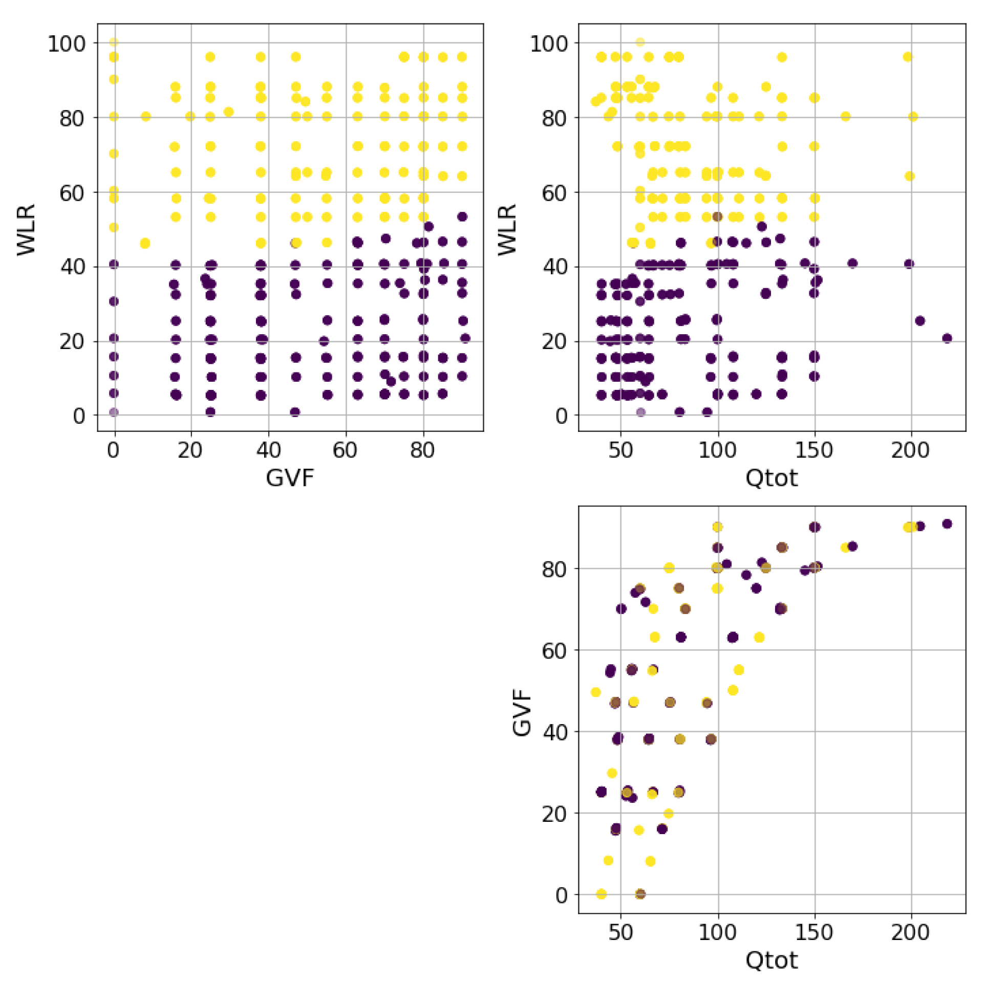
As previously mentioned in Section 4, the data came from an acquisition campaign that took place in the ProLabNL high-pressure flow loop. The data were sampled using the experimental grid shown in Figure 1 and consisted of about 300 experiments with 5 min of recording each and varying flow conditions. These were controlled by three main parameters, which were the GVF, the total flow rate , and WLR, the target of the estimation model. The conditions depicted in the grid were often called multiphase conditions, as opposed to wet gas conditions, which refer to situations where the GVF exceeds 90%.
Depending on the fluid properties, the dataset could be divided into two parts: When the flow was mainly composed of water and the mixture was conductive, the fluid was called water continuous; on the contrary, when the isolating fluids (oil and gas) were the majority, the fluid was called oil continuous, and no conductivity could be measured. The transition between these conditions can be appreciated in Figure 1, where it is clear that WLR is the main parameter controlling this effect, and Qtot does so only weakly. Unfortunately, these fluid properties needed two mutually exclusive measuring instruments to be implemented, one for the conductive regime and another for the capacitive regime where no fluid conduction can measured. This led to the development of two estimators based on the two dataset partitions—water continuous and the oil continuous—with, respectively, about 130 and 170 experiments.
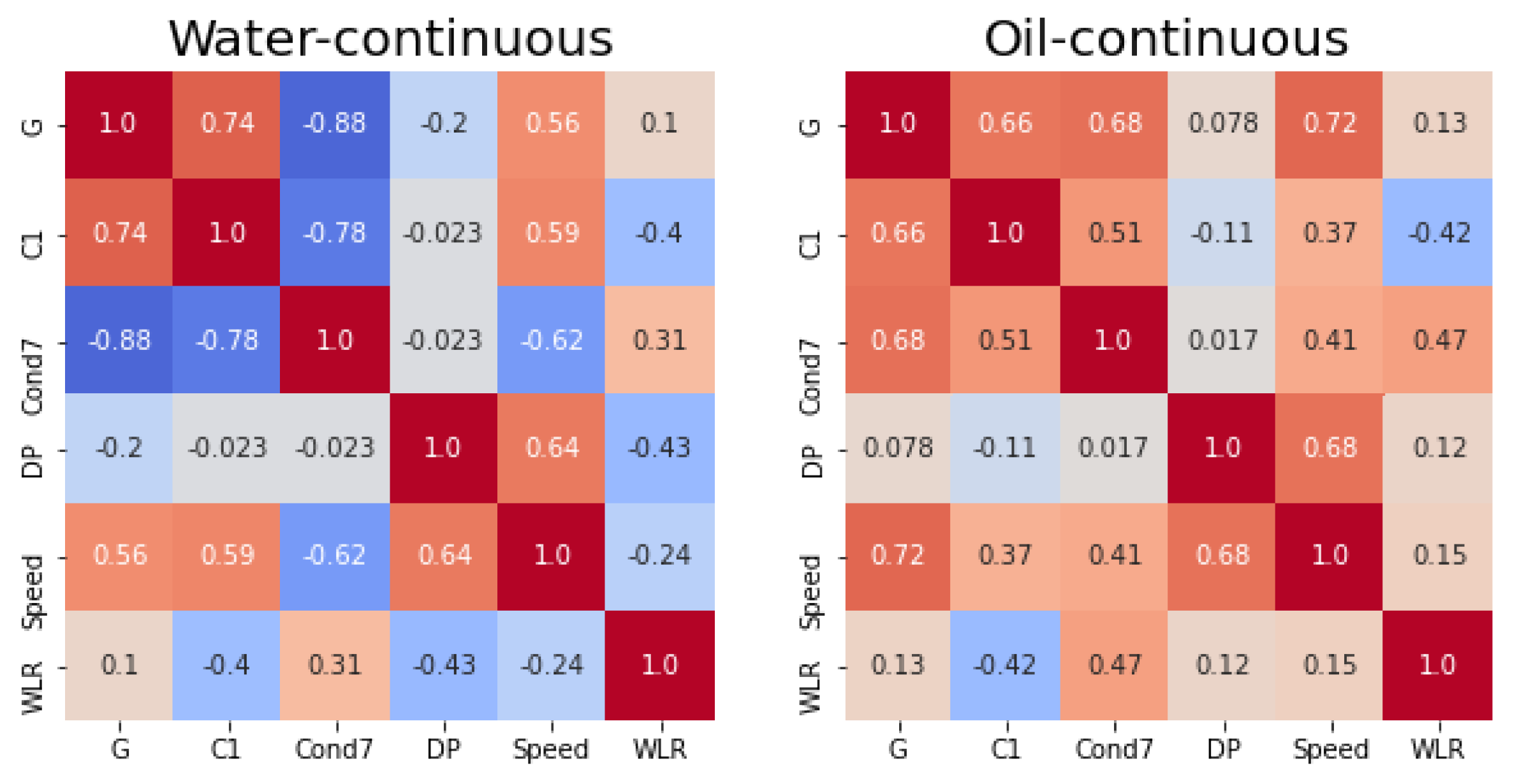
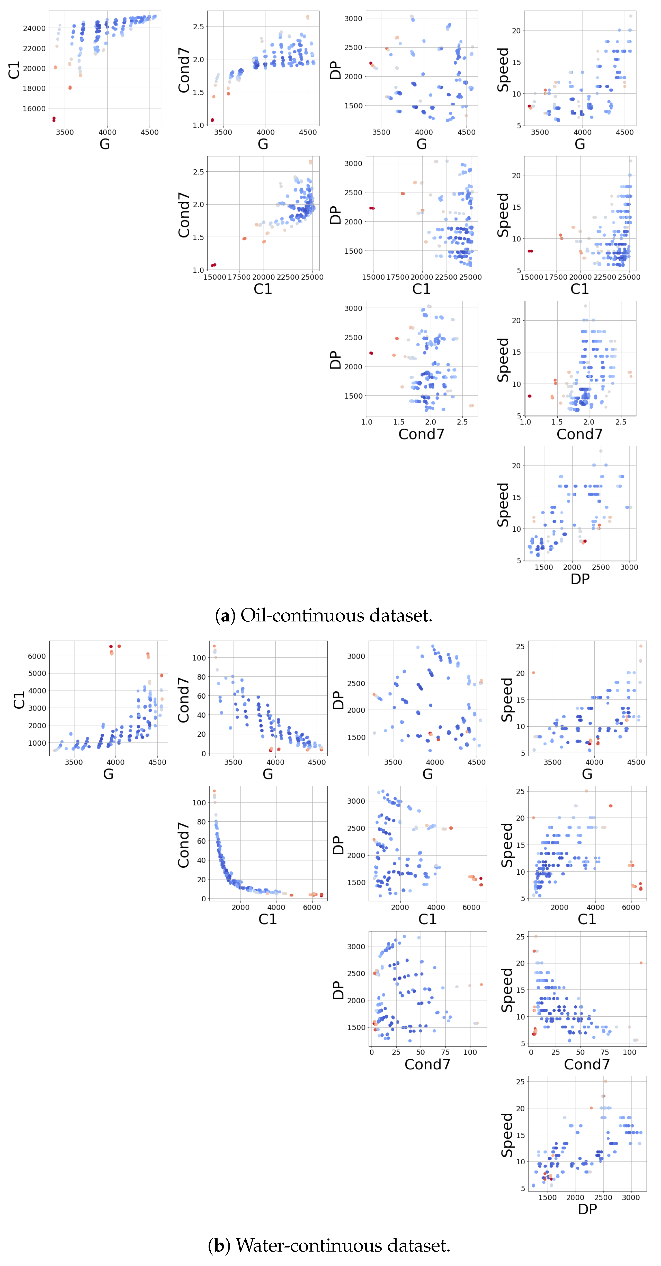
The input sensors collected a stream of measurements with a high frequency rate. Features were extracted from these signals every minute and were then collected in a 5 min array. Once this array was full, the median value of each feature was stored and used for the flow estimation. This procedure allowed us to obtain robust features that were seldom corrupted by anomalous behaviors of the instrumentation. The extracted features were computationally efficient functions that could be easily computed on the device. An example of the stored data is depicted in Figure 3, where one feature is shown for each sensor. To grasp the linear relation between the variables, the Pearson correlation coefficient is plotted in Figure 2.
Despite the efforts to get robust measurements of the fluid proprieties, some flow conditions are very difficult to sample, and the resulting measurements exhibit anomalous behaviors. To overcome this issue and to train and test the model on reliable data, an additional preprocessing step was implemented. This consisted of the application of anomaly detection techniques in order to highlight experiments that may have aroused the suspicion of having been measured with malfunctioning sensors. The tool employed in this context was an isolation forest [50], a powerful and popular method for detecting anomalous data points in an unsupervised manner. The isolation forest is a collection of trees that randomly partition the feature space, isolating the samples. The most anomalous data tend to be isolated faster than the normal ones and are, therefore, more easily detected. This algorithm has many nice properties, such as the fast inference time, which allows this model to be implemented on board and to check if the incoming data are anomalous or not. Figure 3 shows the application of this algorithm to the two datasets. To each data point, the IF associates a score proportional to the abnormality level of the point. This procedure highlights that in some water-continuous experiments, the impedance module exhibits severely abnormal behaviors, which was subsequently confirmed by domain experts. To avoid unreliable results, these anomalous samples were dropped in the last preprocessing step; on the contrary, the oil-continuous data were considered to be sufficiently clean already.
At this point, the main dataset was divided into two smaller datasets containing all of the features extracted by each experiment. This meant that, in the next phase, two models were developed, one for each dataset. The selected model was the one that minimized the mean absolute error (MAE) over 10 repetitions of training and testing, where the test set was composed of 30% of the randomly shuffled total dataset—paying attention to avoid taking training and testing points that were too close—and with the same procedure, the root mean squared error (RMSE) and the 95th percentile of the residuals (95th percentile) were also computed. In order to have a fair evaluation of the generalization capabilities, we carefully handled the training–test split in order to avoid having experiments with very similar settings (GVF, WLR, Qtot) in the different splits. As can be seen from Figure 1, some data points were almost overlapping, and using training and testing points that were too similar would result in an unfair evaluation. To overcome this issue, the points that were closer than 1% GVF, 1% WLR, and 10 are grouped together and put either in the training or in the testing set, not in both.
As mentioned in Section 3, in this work, four models that can provide confidence intervals for the estimated quantity were tested: the feed-forward neural network (FNN), the linear local forest (LLF), the Gaussian process (GP), and the random forest (RF). Since the GP is quite sensitive to the kernel choice, it was tuned according a five-fold cross-validation, testing different combinations of polynomial and radial basis function kernels with different hyper-parameters. On a similar five-fold cross-validation, the RF and LLF proved to be less sensitive to the parameter choice. Concerning the FNN, given the complexity of the training and the complexity of the search space, some design choices were made: the activation functions and the employed learning rate (equal to 0.001) were the ones suggested by typical choices in the literature, and they were not cross-validated; the number of layers was cross-validated five-fold. The number of layers tested was in the range from 3 to 7; in this case, the number of neurons was adapted according to the popular design guidelines reported before with neurons, where d is the number of layers and input features.
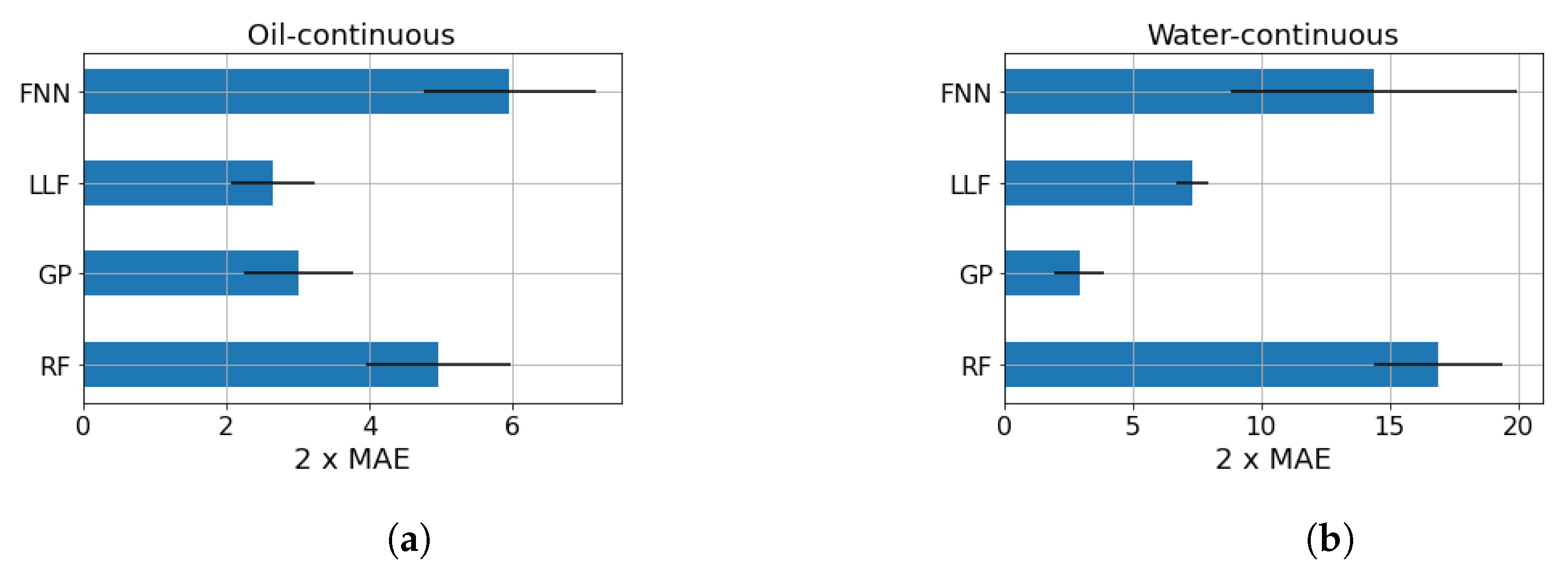
Figure 4 shows the mean results obtained by the procedure described above, together with their standard deviations. In the oil-continuous case, looking only at the mean MAE score, the LLF seems to be the best predictive model; however, the very large error bar suggests that the LLF and GP might be equivalent in a statistical sense. On the contrary, in the water-continuous dataset, the clear winner is the GP, which has much better performance in comparison with the competitors. These results are consistent with what can be expected with the dataset size. The GP has a few parameters to be tuned with respect to the other models, while the RF and FNN suffer from the lack of data. Despite the similarity of the LLF to RF, this method makes stronger assumptions that, in this context, improve its learning ability. More detailed results are shown in Table 1 and Table 2, where the mean results in terms of MAE, RMSE, and 95th percentile are compared. The choice of showing all of these scores and not just the RMSE is due to the presence of outliers. Indeed, in some cases, this score is not reliable, and a more fair index might be the MAE or 95th percentile.
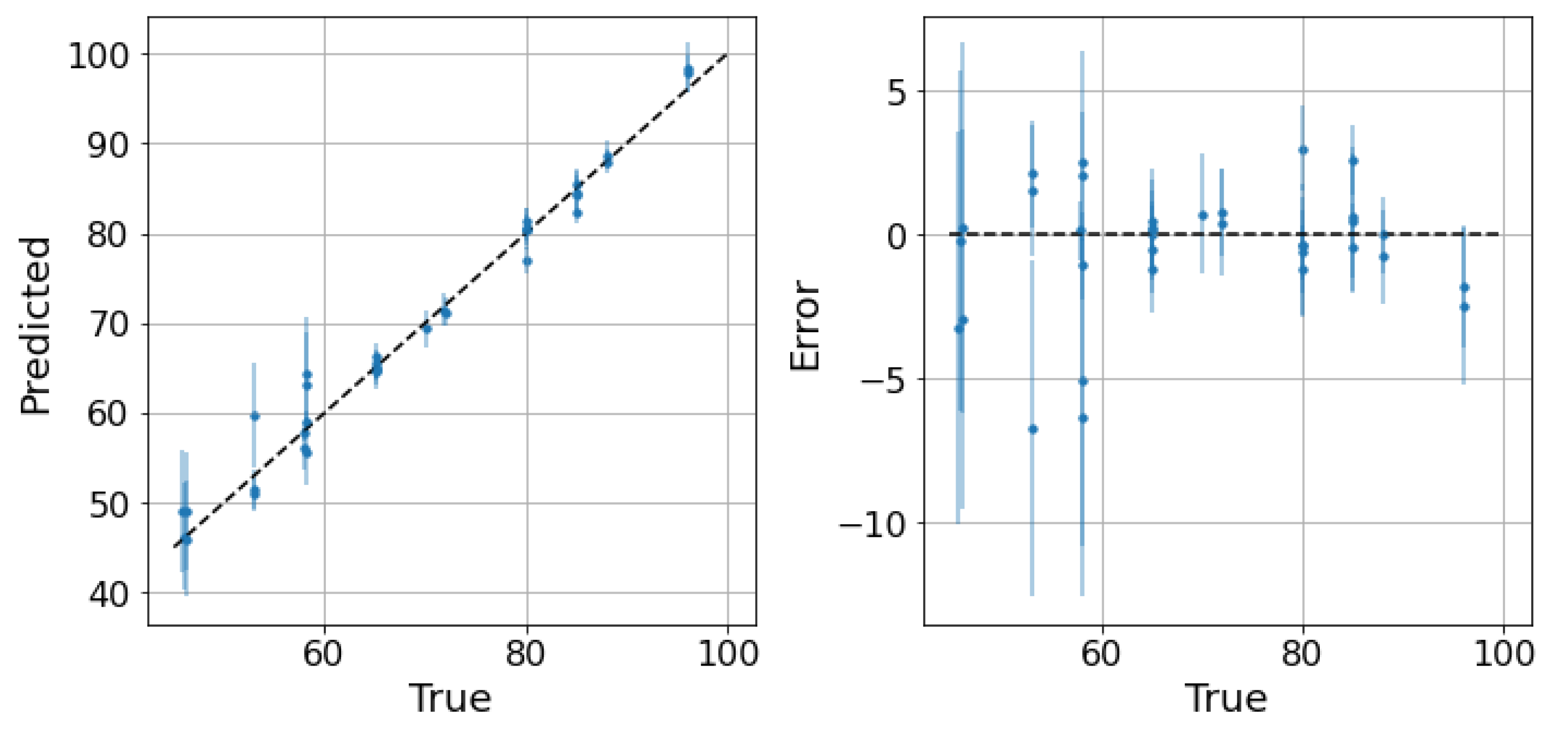
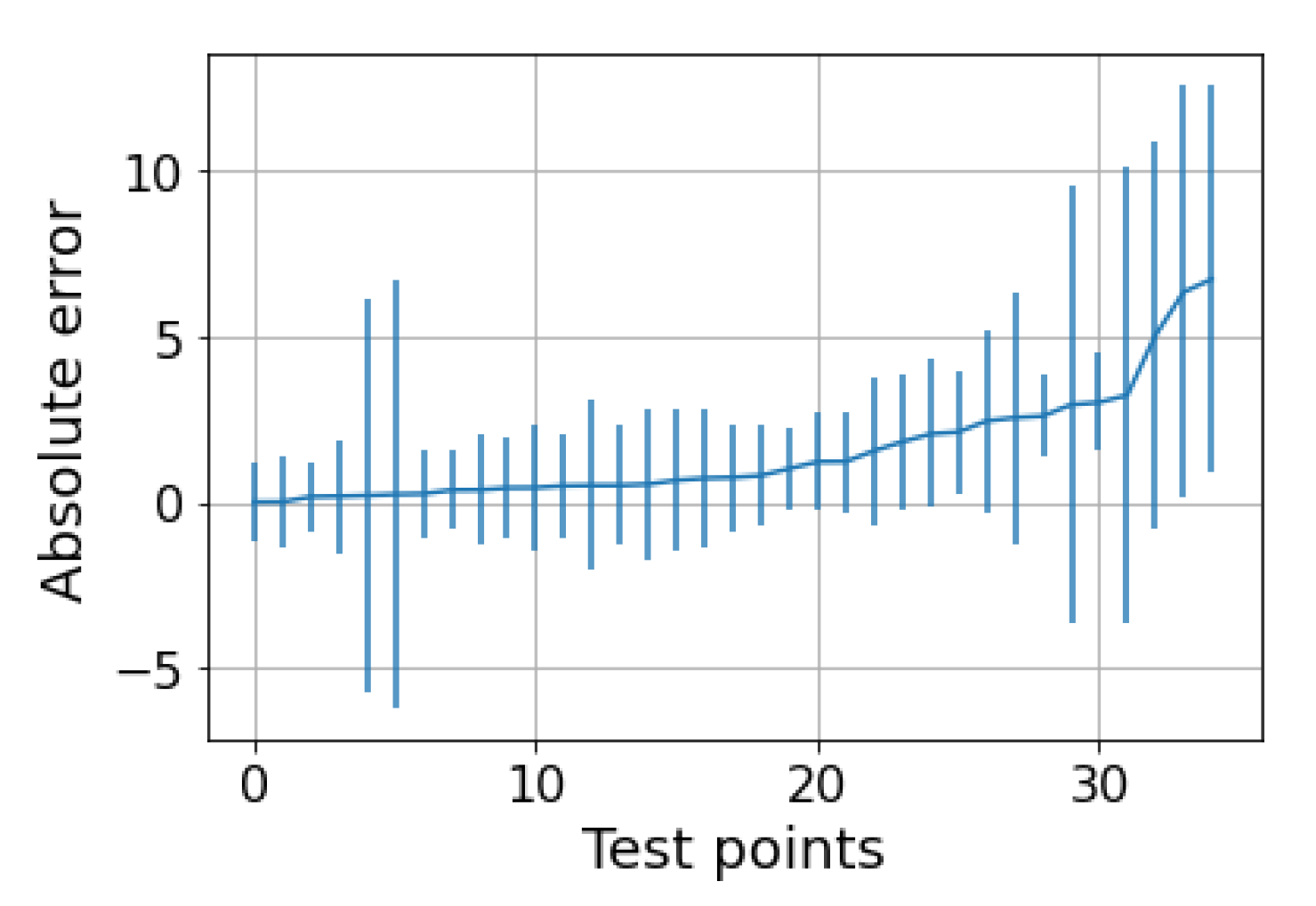
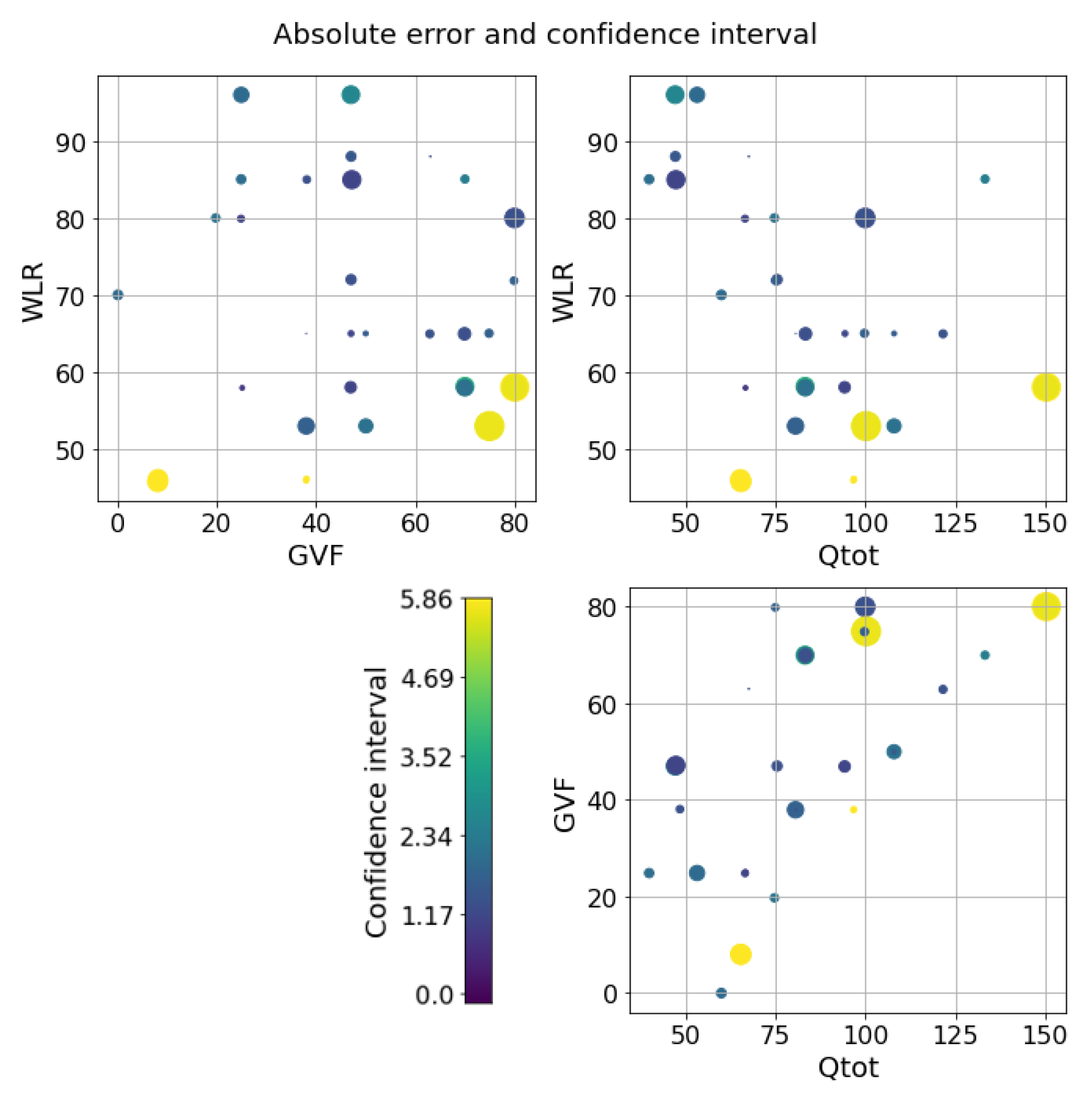
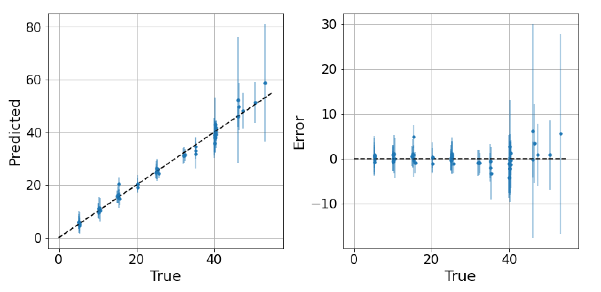
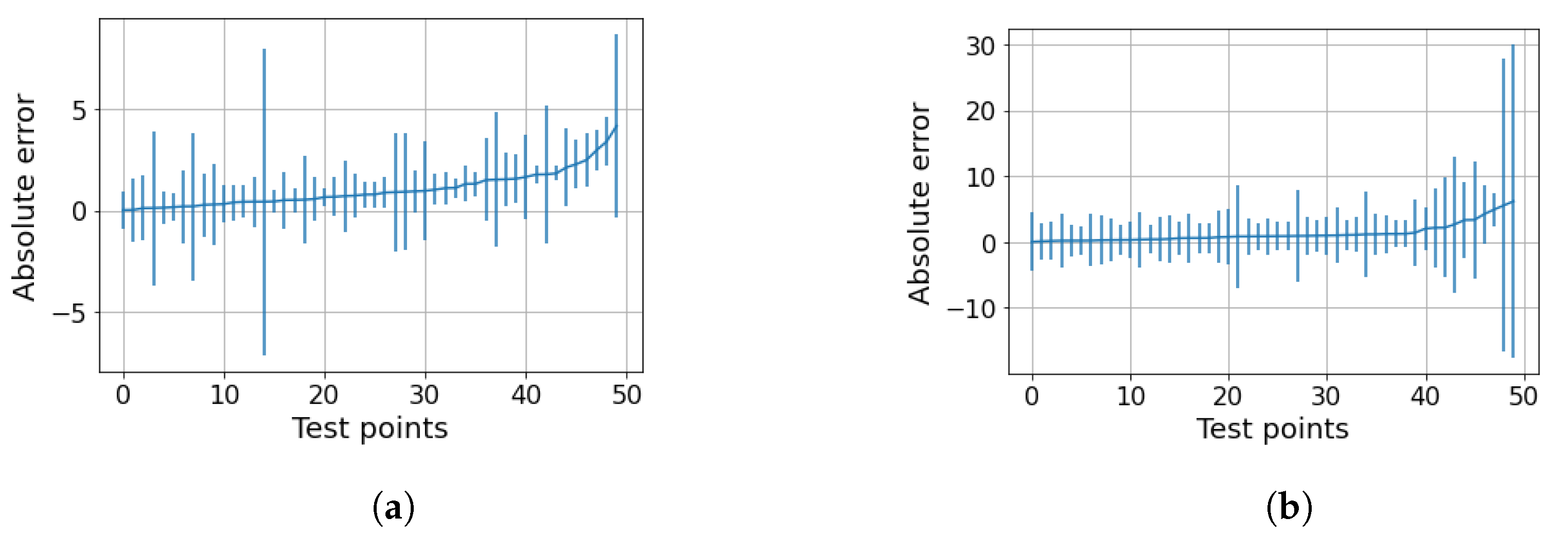
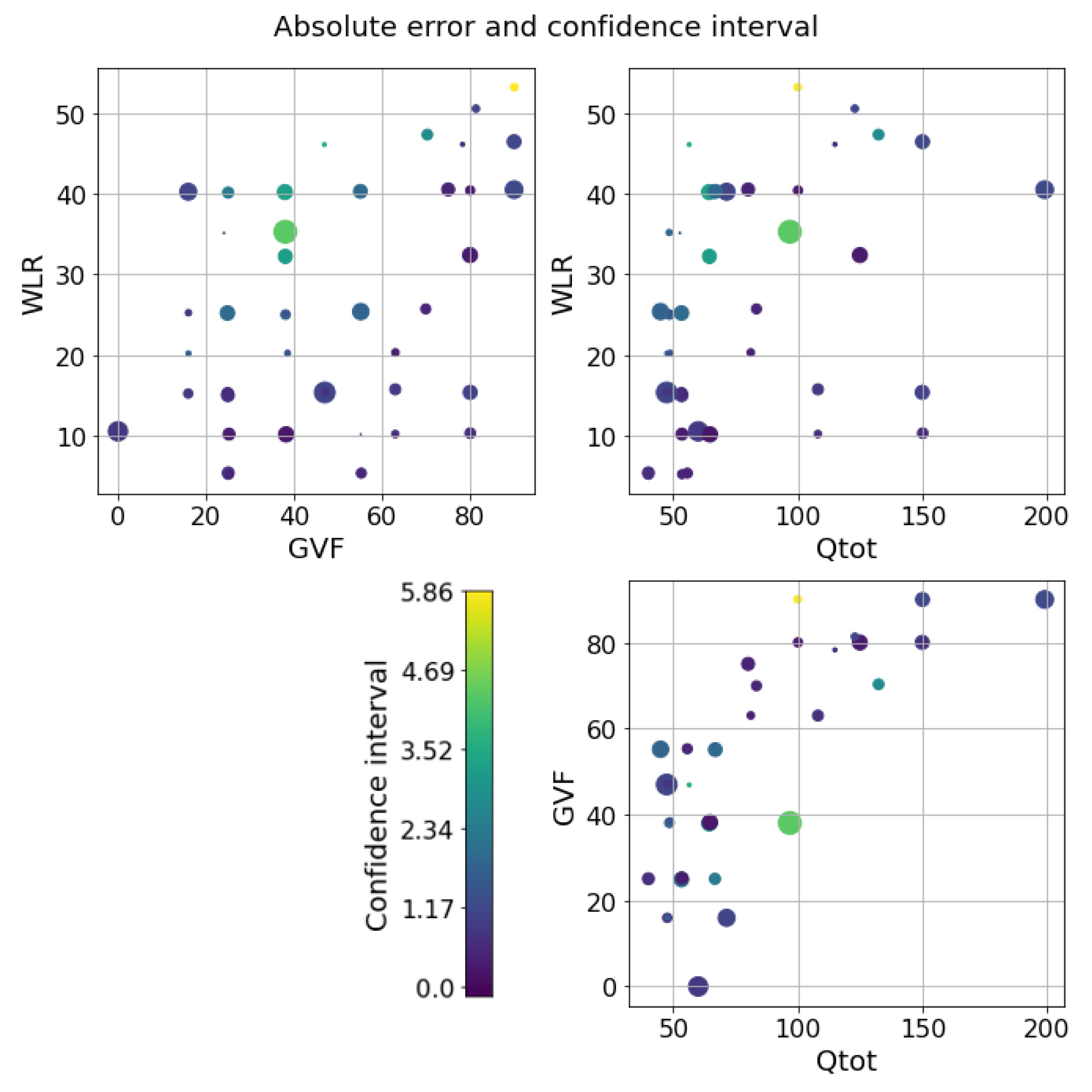
The next step is to test the ability of the selected models to provide reliable confidence intervals for the two datasets. Starting from the water-continuous dataset, the GP was trained and tested on randomly generated partitions, and the results are depicted in Figure 5, Figure 6 and Figure 7. The first figure shows the predicted versus the actual values and the residuals versus the actual values. It confirms the good results expected in the previous test. Indeed, the majority of the test points are close to the bisector, and only a few points are poorly estimated. Here, a zone where the model struggles to predict the correct value and where its confidence intervals are wider starts to appear; it is close to the transition line at 40–60% WLR. The sorted errors with their related intervals are visible in Figure 6. It is interesting to note here that, on average, the confidence intervals get wider as the errors increase, which is an appealing effect for practitioners that may easily neglect predictions with low confidence levels. However, some confidence intervals are quite large even if the prediction error is low, such as in Figure 6. For this situation, it is possible to find a partial explanation by looking at the more complex plot in Figure 7. Here, the test points are shown in the flow parameter space with a size proportional to the error and a color proportional to the confidence interval. It is interesting to note that the points where the prediction is less accurate are the ones that are close to the boundary where the model may suffer from boundary effects, and the instruments are more severely challenged by the extreme working conditions. Moreover, the points close to the transition boundary at around 50% WLR are the ones for which the model returns the most uncertain estimates.
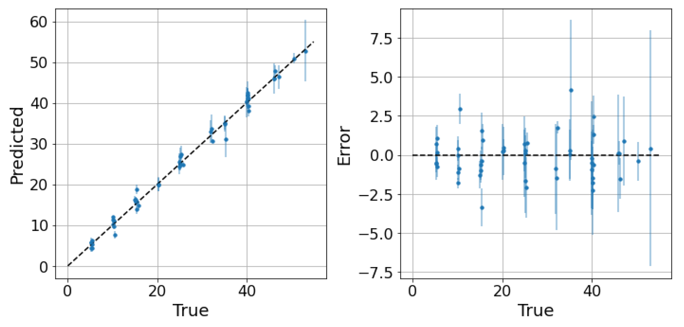
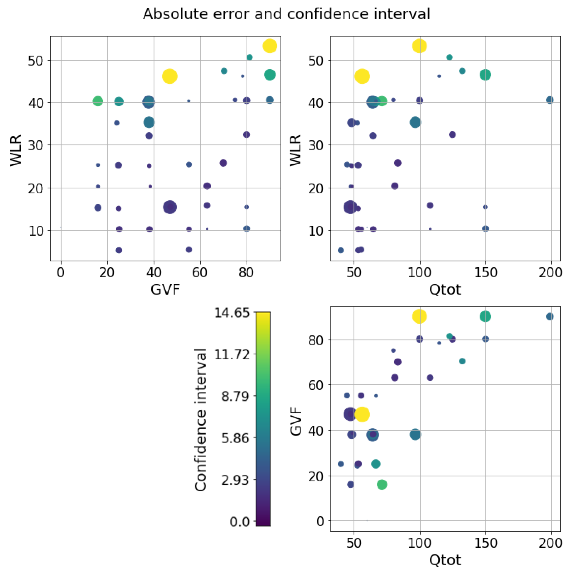
Concerning the oil dataset, as previously explained, the best model is not clear because the performance of the LLF and GP is very close. To understand which model is preferable, the behavior of the confidence intervals may be be helpful. The application of the LLF to a randomly partitioned test set is shown in Figure 8, while the application of the GP is shown in Figure 9. The prediction performance of the GP is slightly worse than that of LLF, as expected, but the great diversity is in the confidence intervals (Figure 10a,b). Indeed, the intervals of the LLF are much shorter (1.59 on average) than those of the GP (4.56 on average), but they are not proportional to the error as they are in the GP model; moreover, the percentage of intervals crossing the zero-error line (the PICP) is quite different: 0.64 against 0.98. The choice of which model to choose may depend on the specific application, since some applications might prefer larger confidence intervals but more certainty, while others prefer smaller intervals but less reliability. Comparing the two models in the flow parameter space, it is possible to see a pattern similar to the one previously described, but only only in the case of the GP (Figure 11 and Figure 12). The majority of the uncertainty, together with the largest error, is clustered close to the transition zone. In conclusion, even if the GP is less accurate than the LLF, it seems to have confidence intervals that are more in line with what can be expected from a physical model.
6. Conclusions
This study applied uncertainty quantification techniques to the estimation of extraction performance in oil and gas production. The extraction performance depends on three indicators that summarize the liquid fraction, the gas fraction, and the total flow of the extracted mixture of oil, gas, and water. This work mainly focused on the water-in-liquid ratio, i.e., the fraction of water inside the total volume of liquid, since it is the most important and most complex among the discussed parameters when the final target is the extraction efficiency.
Four models were tested in order to understand their behavior in this particular context in terms of both prediction accuracy and uncertainty estimation. These models were a feed-forward neural network, Gaussian process, linear local forest, and random forest, and they were applied to two complementary datasets that were previously preprocessed using the isolation forest anomaly detection algorithm. These data came from a particular instrument called a multiphase flow meter, which is used to extract information about the flow and to provide the extraction parameters.
The results show that, most of the time, the Gaussian process is the preferable model, since it has a low error compared to the other methods and a good ability to handle uncertainty. In fact, in this context, it returned confidence intervals proportional to the prediction error. Moreover, it estimated uncertainties that were in accordance with what domain experts would expect. When data are more uncertain, such when the flow is highly non-stationary in the transition regions between two flow conditions, it returns a higher uncertainty. However, another model called the linear local forest proved its potential to make accurate predictions with small amounts of data. The main differences between these two models resulted in the differences in their confidence intervals; while the linear local forest had shorter confidence intervals at the cost of excluding the true value more often, the Gaussian process tended to have wider uncertainties.
Future works should focus on data collection; indeed, it is likely that with more data, the performance of all methods will improve, especially that of random forests and neural networks. In this context, one research direction that the authors are currently investigating is the application of active learning algorithms, which are able to lessen the need for big datasets while improving the predictions.
Author Contributions
Conceptualization, L.F., T.B., E.F. and G.A.S.; methodology, L.F.; software, L.F. and T.B.; validation, T.B. and E.F.; formal analysis, L.F.; investigation, L.F.; resources, E.F. and G.A.S.; data curation, L.F. and E.F.; supervision, E.F. and G.A.S. All authors have read and agreed to the published version of the manuscript.
Funding
Part of this work was supported by MIUR (Italian Ministry for Education) under the initiative “Departments of Excellence” (Law 232/2016). Pietro Fiorentini S.p.A. is gratefully acknowledged for the financial support of this research.
Institutional Review Board Statement
Not applicable.
Informed Consent Statement
Not applicable.
Data Availability Statement
The data that support the findings of this study are available from Pietro Fiorentini S.p.A. but restrictions apply to the availability of these data, which were used under license for the current study, and so are not publicly available.
Conflicts of Interest
The authors declare no conflict of interest.
References
- Market Report: Oil 2021. Available online: https://www.iea.org/reports/oil-2021 (accessed on 1 September 2021).
- Datta, D.; Mishra, S.; Rajest, S.S. Quantification of tolerance limits of engineering system using uncertainty modeling for sustainable energy. Int. J. Intell. Netw. 2020, 1, 1–8. [Google Scholar] [CrossRef]
- Paziresh, M.; Jafari, M.A.; Feshari, M. Confidence Interval for Solutions of the Black-Scholes Model. Adv. Math. Financ. Appl. 2019, 4, 49–58. [Google Scholar]
- Tang, N.S.; Qiu, S.F.; Tang, M.L.; Pei, Y.B. Asymptotic confidence interval construction for proportion difference in medical studies with bilateral data. Stat. Methods Med. Res. 2011, 20, 233–259. [Google Scholar] [CrossRef] [PubMed]
- Council, N.R. Assessing the Reliability of Complex Models: Mathematical and Statistical Foundations of Verification, Validation, and Uncertainty Quantification; The National Academies Press: Washington, DC, USA, 2012. [Google Scholar] [CrossRef]
- Hansen, L.S.; Pedersen, S.; Durdevic, P. Multi-phase flow metering in offshore oil and gas transportation pipelines: Trends and perspectives. Sensors 2019, 19, 2184. [Google Scholar] [CrossRef] [PubMed] [Green Version]
- Thorn, R.; Johansen, G.A.; Hjertaker, B.T. Three-phase flow measurement in the petroleum industry. Meas. Sci. Technol. 2012, 24, 012003. [Google Scholar] [CrossRef]
- Bikmukhametov, T.; Jäschke, J. First principles and machine learning virtual flow metering: A literature review. J. Pet. Sci. Eng. 2020, 184, 106487. [Google Scholar] [CrossRef]
- Sircar, A.; Yadav, K.; Rayavarapu, K.; Bist, N.; Oza, H. Application of machine learning and artificial intelligence in oil and gas industry. Pet. Res. 2021. [Google Scholar] [CrossRef]
- Zambonin, G.; Altinier, F.; Beghi, A.; Coelho, L.d.S.; Fiorella, N.; Girotto, T.; Rampazzo, M.; Reynoso-Meza, G.; Susto, G.A. Machine learning-based soft sensors for the estimation of laundry moisture content in household dryer appliances. Energies 2019, 12, 3843. [Google Scholar] [CrossRef] [Green Version]
- Musil, F.; Willatt, M.J.; Langovoy, M.A.; Ceriotti, M. Fast and accurate uncertainty estimation in chemical machine learning. J. Chem. Theory Comput. 2019, 15, 906–915. [Google Scholar] [CrossRef] [Green Version]
- Imbalzano, G.; Zhuang, Y.; Kapil, V.; Rossi, K.; Engel, E.A.; Grasselli, F.; Ceriotti, M. Uncertainty estimation for molecular dynamics and sampling. J. Chem. Phys. 2021, 154, 074102. [Google Scholar] [CrossRef]
- Tian, Y.; Yuan, R.; Xue, D.; Zhou, Y.; Ding, X.; Sun, J.; Lookman, T. Role of uncertainty estimation in accelerating materials development via active learning. J. Appl. Phys. 2020, 128, 014103. [Google Scholar] [CrossRef]
- Li, Y.; Gao, Z.; He, Z.; Zhuang, Y.; Radi, A.; Chen, R.; El-Sheimy, N. Wireless fingerprinting uncertainty prediction based on machine learning. Sensors 2019, 19, 324. [Google Scholar] [CrossRef] [Green Version]
- Ani, M.; Oluyemi, G.; Petrovski, A.; Rezaei-Gomari, S. Reservoir uncertainty analysis: The trends from probability to algorithms and machine learning. In Proceedings of the SPE Intelligent Energy International Conference and Exhibition, OnePetro, Aberdeen, Scotland, UK, 6–8 September 2016. [Google Scholar]
- Alizadehsani, R.; Roshanzamir, M.; Hussain, S.; Khosravi, A.; Koohestani, A.; Zangooei, M.H.; Abdar, M.; Beykikhoshk, A.; Shoeibi, A.; Zare, A.; et al. Handling of uncertainty in medical data using machine learning and probability theory techniques: A review of 30 years (1991–2020). Ann. Oper. Res. 2021, 1–42. [Google Scholar] [CrossRef]
- Yan, Y.; Wang, L.; Wang, T.; Wang, X.; Hu, Y.; Duan, Q. Application of soft computing techniques to multiphase flow measurement: A review. Flow Meas. Instrum. 2018, 60, 30–43. [Google Scholar] [CrossRef]
- Gel, A.; Garg, R.; Tong, C.; Shahnam, M.; Guenther, C. Applying uncertainty quantification to multiphase flow computational fluid dynamics. Powder Technol. 2013, 242, 27–39. [Google Scholar] [CrossRef]
- Hu, X. Uncertainty Quantification Tools for Multiphase Gas-Solid Flow Simulations Using MFIX. Ph.D. Thesis, Iowa State University, Ames, IA, USA, 2014. [Google Scholar]
- Zhang, X.; Xiao, H.; Gomez, T.; Coutier-Delgosha, O. Evaluation of ensemble methods for quantifying uncertainties in steady-state CFD applications with small ensemble sizes. Comput. Fluids 2020, 203, 104530. [Google Scholar] [CrossRef] [Green Version]
- Valdez, A.R.; Rocha, B.M.; Chapiro, G.; dos Santos, R.W. Uncertainty quantification and sensitivity analysis for relative permeability models of two-phase flow in porous media. J. Pet. Sci. Eng. 2020, 192, 107297. [Google Scholar] [CrossRef]
- Roshani, G.; Nazemi, E.; Roshani, M. Intelligent recognition of gas-oil-water three-phase flow regime and determination of volume fraction using radial basis function. Flow Meas. Instrum. 2017, 54, 39–45. [Google Scholar] [CrossRef]
- AL-Qutami, T.A.; Ibrahim, R.; Ismail, I.; Ishak, M.A. Radial basis function network to predict gas flow rate in multiphase flow. In Proceedings of the 9th International Conference on Machine Learning and Computing, Singapore, 24–26 February 2017; pp. 141–146. [Google Scholar]
- Zhao, C.; Wu, G.; Zhang, H.; Li, Y. Measurement of water-to-liquid ratio of oil-water-gas three-phase flow using microwave time series method. Measurement 2019, 140, 511–517. [Google Scholar] [CrossRef]
- Bahrami, B.; Mohsenpour, S.; Noghabi, H.R.S.; Hemmati, N.; Tabzar, A. Estimation of flow rates of individual phases in an oil-gas-water multiphase flow system using neural network approach and pressure signal analysis. Flow Meas. Instrum. 2019, 66, 28–36. [Google Scholar] [CrossRef]
- Khan, M.R.; Tariq, Z.; Abdulraheem, A. Application of artificial intelligence to estimate oil flow rate in gas-lift wells. Nat. Resour. Res. 2020, 29, 4017–4029. [Google Scholar] [CrossRef]
- Dave, A.J.; Manera, A. Inference of Gas-liquid Flowrate using Neural Networks. arXiv 2020, arXiv:2003.08182. [Google Scholar]
- Zhang, H.; Yang, Y.; Yang, M.; Min, L.; Li, Y.; Zheng, X. A Novel CNN Modeling Algorithm for the Instantaneous Flow Rate Measurement of Gas-liquid Multiphase Flow. In Proceedings of the 2020 12th International Conference on Machine Learning and Computing, Shenzhen, China, 15–17 February 2020; pp. 182–187. [Google Scholar]
- Hu, D.; Li, J.; Liu, Y.; Li, Y. Flow Adversarial Networks: Flowrate Prediction for Gas–Liquid Multiphase Flows Across Different Domains. IEEE Trans. Neural Netw. Learn. Syst. 2019, 31, 475–487. [Google Scholar] [CrossRef]
- Fan, S.; Yan, T. Two-phase air–water slug flow measurement in horizontal pipe using conductance probes and neural network. IEEE Trans. Instrum. Meas. 2013, 63, 456–466. [Google Scholar] [CrossRef]
- Ismail, I.; Gamio, J.; Bukhari, S.A.; Yang, W. Tomography for multi-phase flow measurement in the oil industry. Flow Meas. Instrum. 2005, 16, 145–155. [Google Scholar] [CrossRef]
- Mohamad, E.J.; Rahim, R.; Rahiman, M.H.F.; Ameran, H.; Muji, S.; Marwah, O. Measurement and analysis of water/oil multiphase flow using Electrical Capacitance Tomography sensor. Flow Meas. Instrum. 2016, 47, 62–70. [Google Scholar] [CrossRef]
- Aravantinos, V.; Schlicht, P. Making the relationship between uncertainty estimation and safety less uncertain. In Proceedings of the IEEE 2020 Design, Automation & Test in Europe Conference & Exhibition (DATE), Grenoble, France, 9–13 March 2020; pp. 1139–1144. [Google Scholar]
- Liu, J.Z.; Paisley, J.; Kioumourtzoglou, M.A.; Coull, B. Accurate uncertainty estimation and decomposition in ensemble learning. arXiv 2019, arXiv:1911.04061. [Google Scholar]
- Shrestha, D.L.; Solomatine, D.P. Machine learning approaches for estimation of prediction interval for the model output. Neural Netw. 2006, 19, 225–235. [Google Scholar] [CrossRef]
- Abdar, M.; Pourpanah, F.; Hussain, S.; Rezazadegan, D.; Liu, L.; Ghavamzadeh, M.; Fieguth, P.; Cao, X.; Khosravi, A.; Acharya, U.R.; et al. A review of uncertainty quantification in deep learning: Techniques, applications and challenges. Inf. Fusion 2021, 76, 243–297. [Google Scholar] [CrossRef]
- Vaysse, K.; Lagacherie, P. Using quantile regression forest to estimate uncertainty of digital soil mapping products. Geoderma 2017, 291, 55–64. [Google Scholar] [CrossRef]
- Gal, Y.; Ghahramani, Z. Dropout as a bayesian approximation: Representing model uncertainty in deep learning. In Proceedings of the International Conference on Machine Learning, PMLR, New York City, NY, USA, 19–24 June 2016; pp. 1050–1059. [Google Scholar]
- Goodfellow, I.; Bengio, Y.; Courville, A.; Bengio, Y. Deep Learning; Volume 1, MIT Press: Cambridge, MA, USA, 2016. [Google Scholar]
- Rasmussen, C.E. Gaussian processes in machine learning. In Summer School on Machine Learning; Springer: Berlin, Heidelberg, 2003; pp. 63–71. [Google Scholar]
- Duvenaud, D. Automatic Model Construction with Gaussian Processes. Ph.D. Thesis, Computational and Biological Learning Laboratory, University of Cambridge, Cambridge, UK, 2014. [Google Scholar]
- Friedberg, R.; Tibshirani, J.; Athey, S.; Wager, S. Local linear forests. J. Comput. Graph. Stat. 2020, 30, 503–517. [Google Scholar] [CrossRef]
- Wager, S.; Hastie, T.; Efron, B. Confidence intervals for random forests: The jackknife and the infinitesimal jackknife. J. Mach. Learn. Res. 2014, 15, 1625–1651. [Google Scholar] [PubMed]
- Hastie, T.; Tibshirani, R.; Friedman, J. The Elements of Statistical Learning; Springer Series in Statistics; Springer New York Inc.: New York, NY, USA, 2001. [Google Scholar]
- Breiman, L. Random forests. Mach. Learn. 2001, 45, 5–32. [Google Scholar] [CrossRef] [Green Version]
- Barbariol, T.; Feltresi, E.; Susto, G.A. Self-Diagnosis of Multiphase Flow Meters through Machine Learning-Based Anomaly Detection. Energies 2020, 13, 3136. [Google Scholar] [CrossRef]
- Corneliussen, S.; Couput, J.P.; Dahl, E.; Dykesteen, E.; Frøysa, K.E.; Malde, E.; Moestue, H.; Moksnes, P.O.; Scheers, L.; Tunheim, H. Handbook of Multiphase Flow Metering; Norwegian Society for Oil and Gas Measurement: Olso, Norway, 2005. [Google Scholar]
- Barbosa, C.M.; Salgado, C.M.; Brandão, L.E.B. Study of Photon Attenuation Coefficient in Brine Using MCNP Code; Sao Paulo, Barsil, 2015; Available online: https://core.ac.uk/download/pdf/159274404.pdf (accessed on 23 July 2021).
- ProLabNL. Available online: http://www.prolabnl.com (accessed on 1 September 2021).
- Liu, F.T.; Ting, K.M.; Zhou, Z.H. Isolation forest. In Proceedings of the 2008 Eighth IEEE International Conference on Data Mining, Pisa, Italy, 15–19 December 2008; pp. 413–422. [Google Scholar]
Figure 1.
Experiments making up the dataset. The purple points are the oil-continuous experiments, while the yellow ones are the water-continuous experiments. The WLR and GVF are given in percentages, while Qtot is depicted using auxiliary units.
Figure 1.
Experiments making up the dataset. The purple points are the oil-continuous experiments, while the yellow ones are the water-continuous experiments. The WLR and GVF are given in percentages, while Qtot is depicted using auxiliary units.

Figure 2.
Heat map of the correlation coefficients between the extracted features and WLR.

Figure 3.
Input data and anomaly scores obtained with the isolation forest. The color scale goes from blue to red, where red indicates a higher probability of being an outlier. All of the above data are depicted with auxiliary units.
Figure 3.
Input data and anomaly scores obtained with the isolation forest. The color scale goes from blue to red, where red indicates a higher probability of being an outlier. All of the above data are depicted with auxiliary units.

Figure 4.
Results of the model selection. To be consistent with Table 1 and Table 2, the MAE is reported twice. (a) oil-continuous data; (b) water-continuous data.

Figure 5.
GP on the water dataset. Predictions and related confidence intervals of the Gaussian process. 2 MAE: 3.04, 2 RMSE: 4.53, 95th percentile: 5.41.
Figure 5.
GP on the water dataset. Predictions and related confidence intervals of the Gaussian process. 2 MAE: 3.04, 2 RMSE: 4.53, 95th percentile: 5.41.

Figure 6.
GP on the water dataset. Sorted test points with their related uncertainties. The MPIW is 2.6 and the percentage of intervals crossing the zero-error line (PICP) is 86% compared to the expected 95%.
Figure 6.
GP on the water dataset. Sorted test points with their related uncertainties. The MPIW is 2.6 and the percentage of intervals crossing the zero-error line (PICP) is 86% compared to the expected 95%.

Figure 7.
GP on the water dataset. Errors and confidence intervals over the flow parameter space. The size of the dot is proportional to the error, while the color is proportional to the uncertainty. The color scale goes from purple to yellow.
Figure 7.
GP on the water dataset. Errors and confidence intervals over the flow parameter space. The size of the dot is proportional to the error, while the color is proportional to the uncertainty. The color scale goes from purple to yellow.

Figure 8.
LLF on the oil dataset: predictions and related confidence intervals. 2 MAE: 2.03, 2 RMSE: 2.68, 95th percentile: 2.72.
Figure 8.
LLF on the oil dataset: predictions and related confidence intervals. 2 MAE: 2.03, 2 RMSE: 2.68, 95th percentile: 2.72.

Figure 9.
GP on the oil dataset dataset: predictions and related confidence intervals. 2 MAE: 2.49, 2 RMSE: 3.74, 95th percentile: 4.58.
Figure 9.
GP on the oil dataset dataset: predictions and related confidence intervals. 2 MAE: 2.49, 2 RMSE: 3.74, 95th percentile: 4.58.

Figure 10.
Oil dataset. (a) LLF on the oil dataset. Sorted test points with their related confidence intervals. The MPIW is 1.59 and the percentage of intervals crossing the zero-error line (PICP) is 64 compared to the expected 95%. (b) GP on the oil dataset. Sorted test points with their related confidence intervals. The MPIW is 4.56 and the percentage of intervals crossing the zero-error line (PICP) is 98 compared to the expected 95%.

Figure 11.
LLF on the oil dataset. Errors and confidence intervals over the flow parameter space. The size of the dot is proportional to the error, while the color is proportional to the uncertainty. The color scale goes from purple to yellow.
Figure 11.
LLF on the oil dataset. Errors and confidence intervals over the flow parameter space. The size of the dot is proportional to the error, while the color is proportional to the uncertainty. The color scale goes from purple to yellow.

Figure 12.
GP on the oil dataset. Errors and confidence intervals over the flow parameter space. The size of the dot is proportional to the error, while the color is proportional to the uncertainty. The color scale goes from purple to yellow.
Figure 12.
GP on the oil dataset. Errors and confidence intervals over the flow parameter space. The size of the dot is proportional to the error, while the color is proportional to the uncertainty. The color scale goes from purple to yellow.


Table 1.
Mean results of the water-continuous data. To be consistent with the 95th percentile of the absolute error, the MAE and the RMSE are reported twice.
Table 1.
Mean results of the water-continuous data. To be consistent with the 95th percentile of the absolute error, the MAE and the RMSE are reported twice.
| FNN | GP | LLF | RF | |
|---|---|---|---|---|
| 2 MAE | 14.36 | 2.94 | 7.34 | 16.89 |
| 2 RMSE | 17.60 | 3.89 | 9.66 | 19.96 |
| 95th percentile | 15.79 | 3.86 | 9.68 | 17.24 |
Table 2.
Mean results of the oil-continuous data. To be consistent with the 95th percentile of the absolute error, the MAE and the RMSE are reported twice.
Table 2.
Mean results of the oil-continuous data. To be consistent with the 95th percentile of the absolute error, the MAE and the RMSE are reported twice.
| FNN | GP | LLF | RF | |
|---|---|---|---|---|
| 2 MAE | 5.96 | 3.02 | 2.66 | 4.97 |
| 2 RMSE | 8.13 | 5.47 | 4.27 | 7.42 |
| 95th percentile | 8.20 | 4.87 | 3.57 | 7.07 |
Publisher’s Note: MDPI stays neutral with regard to jurisdictional claims in published maps and institutional affiliations. |
© 2021 by the authors. Licensee MDPI, Basel, Switzerland. This article is an open access article distributed under the terms and conditions of the Creative Commons Attribution (CC BY) license (https://creativecommons.org/licenses/by/4.0/).
Share and Cite
MDPI and ACS Style
Frau, L.; Susto, G.A.; Barbariol, T.; Feltresi, E. Uncertainty Estimation for Machine Learning Models in Multiphase Flow Applications. Informatics 2021, 8, 58. https://0-doi-org.brum.beds.ac.uk/10.3390/informatics8030058
AMA Style
Frau L, Susto GA, Barbariol T, Feltresi E. Uncertainty Estimation for Machine Learning Models in Multiphase Flow Applications. Informatics. 2021; 8(3):58. https://0-doi-org.brum.beds.ac.uk/10.3390/informatics8030058
Chicago/Turabian StyleFrau, Luca, Gian Antonio Susto, Tommaso Barbariol, and Enrico Feltresi. 2021. "Uncertainty Estimation for Machine Learning Models in Multiphase Flow Applications" Informatics 8, no. 3: 58. https://0-doi-org.brum.beds.ac.uk/10.3390/informatics8030058
Note that from the first issue of 2016, this journal uses article numbers instead of page numbers. See further details here.