Implementation of Advanced Demand Side Management for Microgrid Incorporating Demand Response and Home Energy Management System

Abstract

To facilitate the possible technology and demand changes in a renewable-energy dominated future energy system, an integrated approach that involves Renewable Energy Sources (RES)-based generation, cutting-edge communication strategies, and advanced Demand Side Management (DSM) is essential. A Home Energy Management System (HEMS) with integrated Demand Response (DR) programs is able to perform optimal coordination and scheduling of various smart appliances. This paper develops an advanced DSM framework for microgrids, which encompasses modeling of a microgrid, inclusion of a smart HEMS comprising of smart load monitoring and an intelligent load controller, and finally, incorporation of a DR strategy to reduce peak demand and energy costs. Effectiveness of the proposed framework is assessed through a case study analysis, by investigation of DR opportunities and identification of energy savings for the developed model on a typical summer day in Western Australia. From the case study analysis, it is evident that a maximum amount of 2.95 kWh energy can be shifted to low demand periods, which provides a total daily energy savings of 3%. The total energy cost per day is AU$2.50 and AU$3.49 for a house with and without HEMS, respectively. Finally, maximum possible peak shaving, maximum shiftable energy, and maximum standby power losses and energy cost savings with or without HEMS have been calculated to identify the energy saving opportunities of the proposed strategy for a microgrid of 100 houses with solar, wind, and a back-up diesel generator in the generation side.

1. Introduction

Modern electric power systems are going through a revolutionary change because of increasing demand for electric power worldwide. Mounting political pressure, public awareness of reducing carbon emission, incorporations of large-scale renewable power penetration, and blending information as well as communication technologies with power system operation are also the major motives of this revolution [1,2]. These issues initiated the establishment of the microgrid concept, which has gone through major development and changes in the last decade, and recently got a boost in its growth after being blessed by smart grid technologies. Microgrids can enhance local reliability, require lower investment costs, reduce emissions, improve power quality, and reduce the power losses of distribution networks [3,4]. One of the challenges that microgrid systems face is to rely mostly on renewable energy sources and ensure that the usage of heterogeneous energy sources is balanced. However, due to their uncertain and intermittent character, the renewable sources are not easily predictable, and the balancing task becomes less obvious to apply [5].

The suitably combined operation of distributed energy resources (DERs) and advanced demand side management (DSM) in a microgrid constituting of a robust communication scheme can play a pivotal role in reducing energy inefficiency by balancing the supply and demand. Application of the Demand Response (DR) and Home Energy Management System (HEMS) are two important components of DSM. DR refers to actions that either reduce the overall amount of energy consumed or change the shape of the load curve by reducing the load at times of peak demand or by shifting the load into low demand (off-peak) periods [6]. The importance of DR has been studied in microgrid applications in recent years [7,8,9,10,11,12,13,14]. DR programs can be classified into two types: reliability-based (direct load control) and market-based (price-based) programs. DR programs are offered to modify consumers’ energy consumption to provide better grid efficiency [15,16] and encourage consumers to make temporary (short-term) adjustments in their energy demand in response to a direct load control signal or electricity pricing signals from the network operator [11]. Several issues have been studied in this regard, such as: heating-cooling systems as an effective structure in energy management [12]; reserve and energy scheduling methods [13]; and the effects of consumers in all parts of the system, such as carbon production [14].

The HEMS is a technology platform encompassing both software and hardware which allows consumers to monitor the overall load profiles, as well as automatically and/or manually shift and curtail demand to ameliorate total consumption. The HEMS can shift or curtail the load in response to DR signals (DLC (Direct Load Control) or pricing) and according to human comfort to optimize electricity consumption during peak hours or when the network condition is jeopardized [17,18]. Under the sustainable smart grid paradigm, the smart house with its HEMS plays an important role in improving the efficiency, economics, reliability, and energy conservation for distribution systems. A study on HEMS efficiency in [19] indicates that a HEMS can reduce the operational cost of electricity by 23.1% and decrease the residential peak-load demand by 29.6%. In addition, it can be found from [20] that other advantages of a HEMS include the minimization of energy wastage, reduction of household occupant intervention, eco-friendliness, and improvement of resident well-being.

Difficulties may arise for the HEMS to intuitively develop a model that can simultaneously coordinate multiple unique appliances [21]. Several pieces of research with different methodologies have been adopted to deal with efficient energy management for residential environments in microgrids [22,23,24,25,26]. For instance, a multi-objective optimized energy management (MOEMS) model for a residential microgrid, with active participation of both generation and demand sides considering reduced energy costs and users’ comfort levels are presented in [22]. A smart energy management system was considered in [23] with mathematical microgrid models with the master-slave control of distributed generation units. An extensive study of smart energy management systems within a smart microgrid environment consisting of two-way digital communications between utility and household devices has been represented in [24] to improve energy efficiency, consumption behavior, and comfort levels. An optimal hierarchical control strategy for residential DC microgrids has been depicted in [25] where a multi-level optimizer was designed to track the system behavior of controllable energy sources. Another study was performed in [26] to optimize the real-time Energy Management System (EMS) for a residential hybrid AC/DC microgrid with energy storage systems (ESS) where scheduling of the charge/discharge of the ESS and the energy injection/consumption was also implemented.

A few studies, such as [17,27,28,29,30], considered the uncertainties of appliance operational time, intermittent renewable generation, and variations of electricity prices, and have developed stochastic efficient scheduling schemes using the Fuzzy Logic method for HEMSs. In [30], a low-complexity Fuzzy Logic Control (FLC)-based EMS used generation and demand forecasting to anticipate the future behavior of the microgrid. The Fuzzy Logic method is used to convert the legion of data into a smaller set of rules. Since the method is based on heuristics, it has the capability to take into consideration human intuition and experience. In addition, the fuzzy rules and membership functions are very flexible and can be reshaped. Authors in [28] propose a controller based on fuzzy logic to mitigate the energy consumption of the building while respecting consistent consumer comfort. Their proposed controller demonstrates better efficiency in contrast to the typical method for cost saving (almost 20%). The study in [29] proposes a more sophisticated strategy for smart homes that merges a Bluetooth low-energy based wireless network with the home appliances to communicate with a HEMS architecture that was ameliorated by a fuzzy-based approach. Their results illustrate higher efficiency in contribution to comfort levels of the users by putting a limited delay factor on each appliance and decreasing peak demand and overall consumption, hence resulting in significant cost reduction.

The HEMS can be incorporated with DR signals (both pricing and DLC) from utility in order to exchange information for electricity usage scheduling. Incorporating the HEMS with the DR can achieve an optimal power scheduling scheme for each electric appliance. A recent study proposed a conceptual study on Virtual Power Plant (VPP) architecture for energy management of the assets owned by consumers participating in DR programs [31]. The authors proposed a service-oriented approach to implement the optimal management of the consumer’s assets in different forms of DR requests, from Price-Based DRs to Event-Based DRs that was applied in modern distribution networks. Studies in [32,33] developed the HEMS on the basis of DR information from the utility to automatically schedule all appliances in houses in the most cost-effective way. Authors in [34] employed economic theories and mathematical formulations to introduce a new model for time-of-use (TOU)-based DR programs with effective market-oriented DR models for residential consumers to change their time of consumption. Another study has been performed to improve cost-effectiveness and consumer comfort under different pricing schemes and weather conditions formulated with mixed integer nonlinear problems (MINLP) and its performance, tested under different operating scenarios with real data [35].

Based on the aforementioned papers, it is clear that numerous research activities have dealt with several strategies with multiplex methods of residential energy management. However, only the DR pricing signal (real-time pricing) from the utility was considered in those studies, and inclusion of DLC signals into the HEMS from the utility was not studied. Furthermore, the conditions of locally available household supply voltages, such as those provided by a smart meter, were not considered in the control algorithm when appliances were scheduled through a HEMS. Controlling the voltage locally can help to maintain the network voltage within acceptable limits and, at the same time, minimize issues, such as automatic disconnection of the local solar photovoltaics (PV) inverters [36] at consumer premises, network capacity upgrades, and communication burdens between a utility and the HEMS.

Therefore, this study proposes an advanced DSM framework for a microgrid environment, which incorporates smart HEMSs located at consumers’ premises. The developed smart HEMS has the ability to coordinate with DR programs (both dynamic pricing and DLC programs). The main contributions of this paper are summarized as follows:

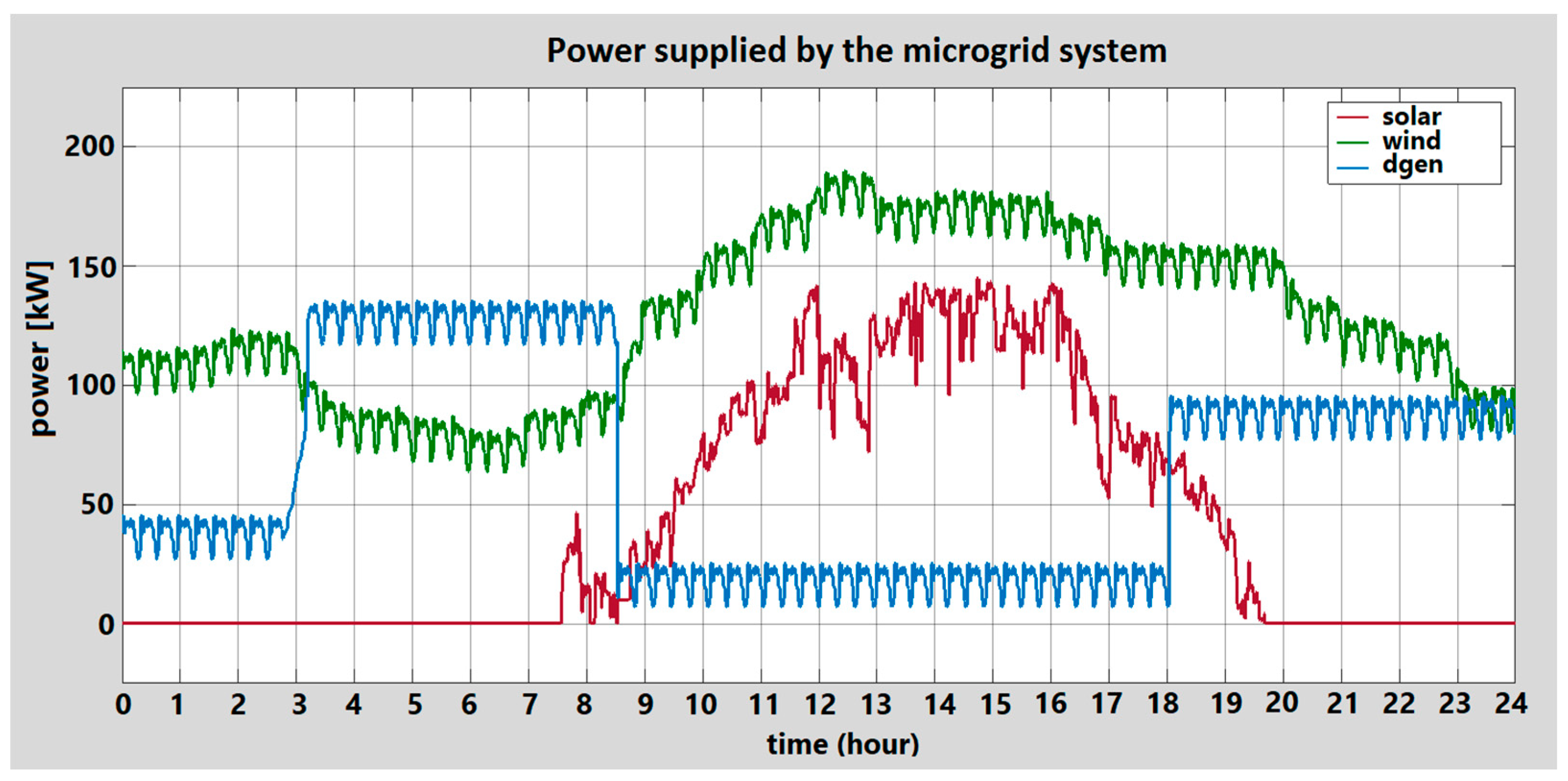
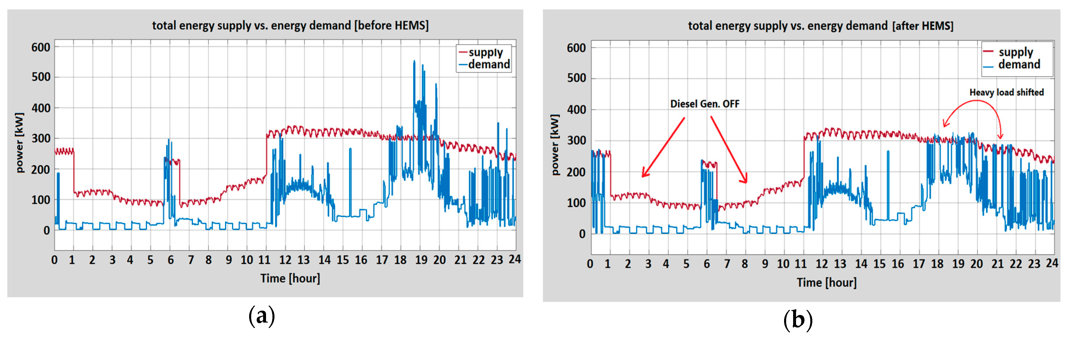
• The proposed DSM framework comprised with advanced communication mediums and HEMSs is tested on a realistic microgrid environment which consists of solar PV, wind, and back-up diesel generators. The developed DSM strategy can maximize the renewable energy usages, maintain supply and demand balance, while reducing the usage of diesel generators in the microgrid.
• The developed smart HEMS in DSM is a fuzzy, logic-based load controller which optimizes household appliances based on the available renewable generation in the microgrid, local voltage measurements from the smart meter, weather conditions (temperature), and consumer consumption preferences, as well as TOU prices and DLC signals from utility.
• The smart HEMS can significantly reduce the consumer’s energy consumption, standby power loss, and energy costs, while maintaining the consumer’s comfort levels.

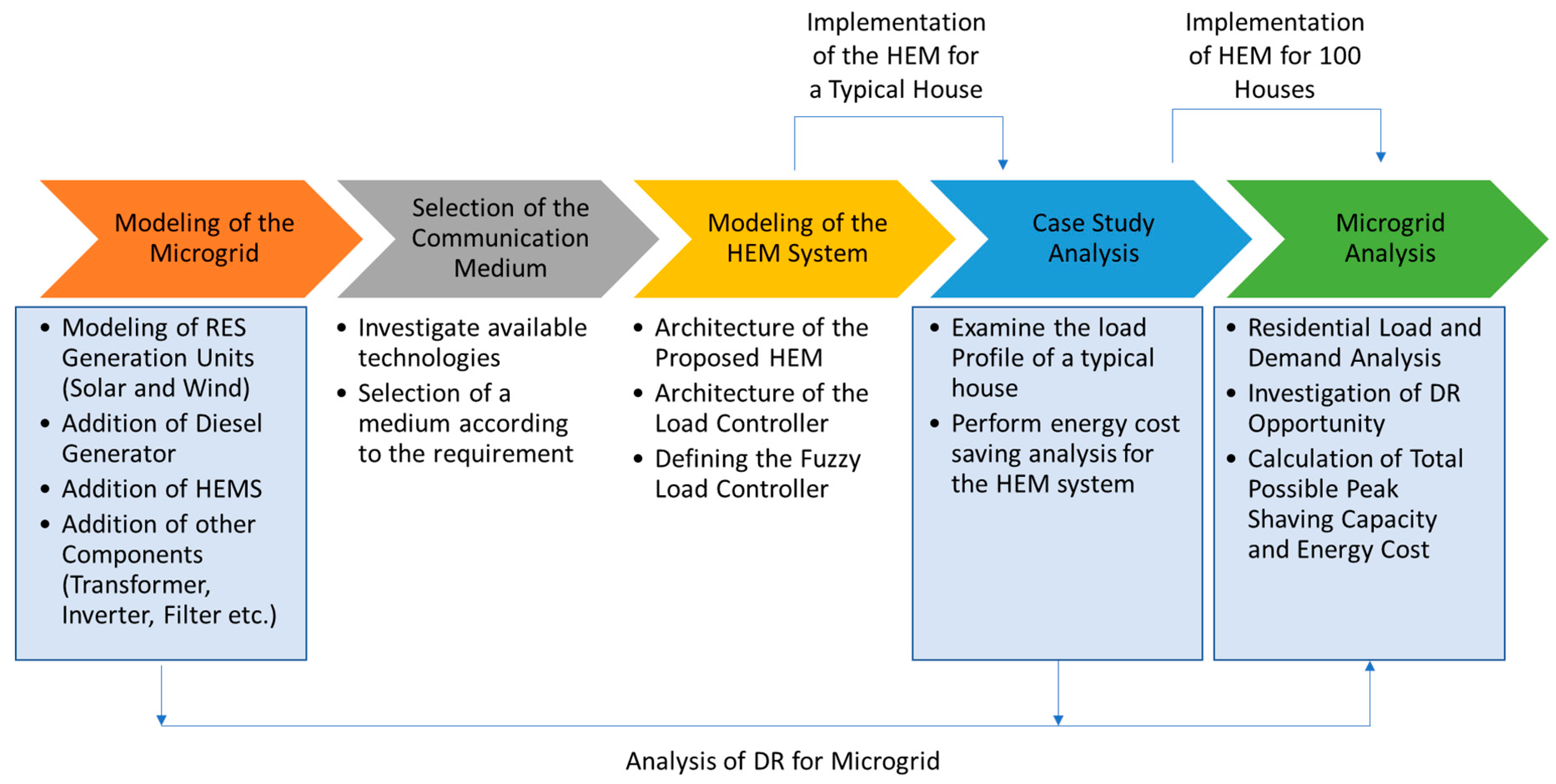
2. Methodology

This study proposes the development of an advanced DSM framework for microgrid-based power systems which consists of smart HEMSs that incorporate DR and has a corresponding communication scheme.

The proposed DSM framework based on a microgrid environment comprises of the following five modules:

(i)

Modeling of Microgrid: A model of a microgrid integrating the solar PV, a wind turbine, and a diesel generator supplying several typical households that participate in DR incorporated with a smart load controller system has been developed.

(ii)

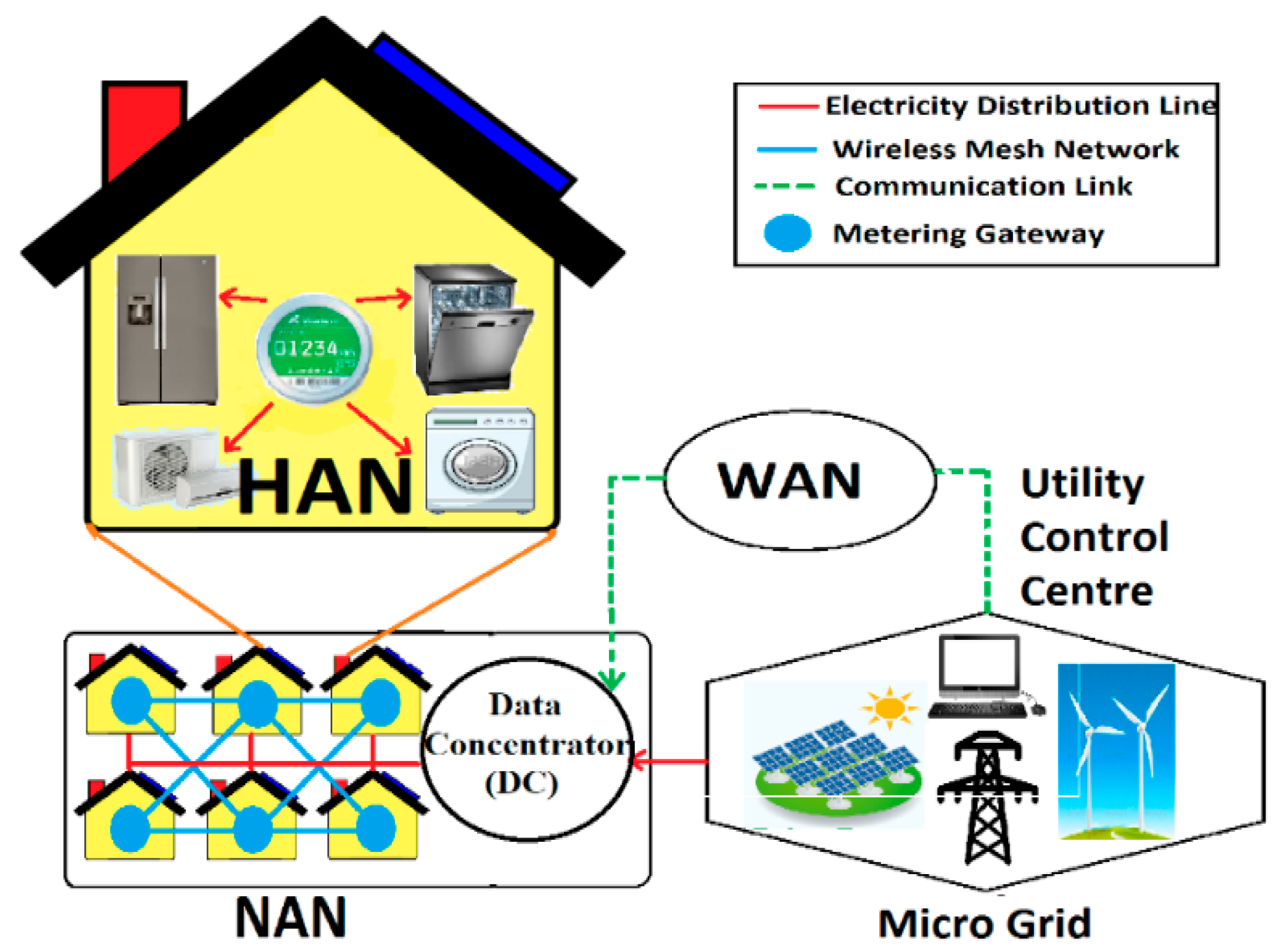
Selection of Communication Medium: The most suitable communication infrastructure for DR and HEMS implementation is selected based on the literature review and geographic position of the community.

(iii)

Modeling of the Smart HEMS: A smart HEMS is developed based on realistic load profiles and appliances’ consumption data obtained from a smart load monitoring device installed in the end-users’ premises. The developed HEMS provides consumption decisions based on predefined fuzzy logic rules. The fuzzy rules are defined according to consumer consumption priorities, local voltage levels, total renewable generation in the microgrid, DR signals (dynamic pricing and DLC), and weather conditions.

(iv)

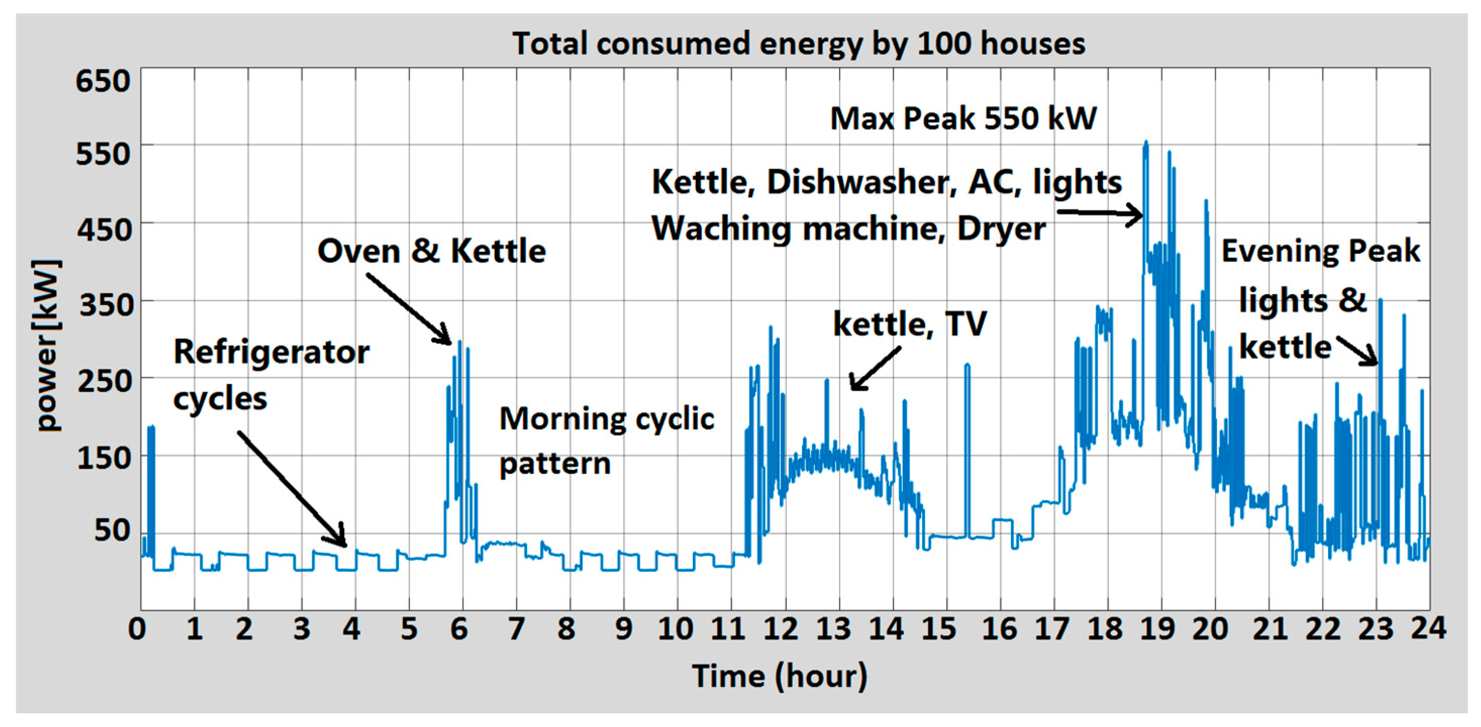
Case Study Analysis: The effectiveness of the proposed framework is evaluated through a case study analysis. The renewable energy sources and domestic loads have been designed based on realistic data of a region in Western Australia, which helps in determining the potential DR opportunity and standby power consumption of major appliances, including refrigerators, air conditioners (AC), dish washers, washing machines and dryers.

(v)

Microgrid Analysis with HEMS: DR opportunities are investigated and identify energy savings for a microgrid system with HEMSs.

Figure 1 shows the step-by-step methodology of this study. Figure 2 shows the overall architecture of the proposed DSM system for the microgrid and the required communication infrastructure between residential consumers and the utility data center, which consists of the Home Area Network (HAN), Neighborhood Area Network (NAN), and Wide Area Network (WAN). The comprehensive framework yields a sensible and simplified platform that can incorporate the HEMS and DR for the microgrid DSM implementation.

3. Modeling of the Microgrid

In order to model the microgrid, it has been considered that there will be two RES-based plants, namely solar and wind. A diesel generator will be used as a back-up resource to ensure the reliability of the system. It is also considered that there are 100 consumers on the distribution side of the grid. Considering these facts, the microgrid has been modeled in Simulink (MATLAB) and includes a 150 kW solar PV farm, a 200 kW wind farm, and a 150 kW diesel generator in the generation side with all their functional controllers, converters, and transformers. The power is being supplied to multiple residential loads, each with several home appliances and a HEMS. The developed model is shown in Figure 3.

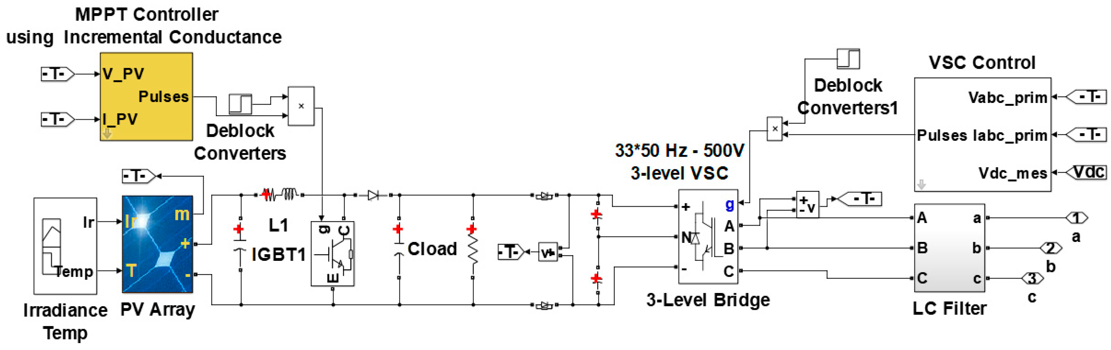
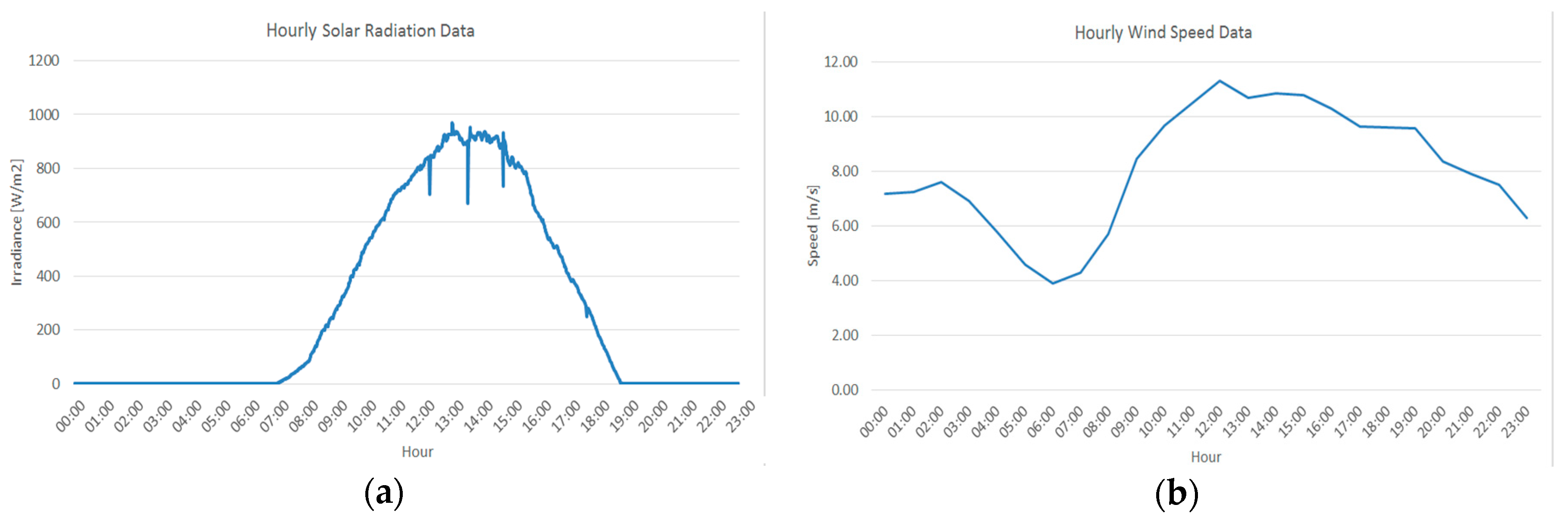
3.1. Modeling of Solar PV

In this study, a SunPower SPR-305E-WHT-D PV module was used, containing 25 cells in series and 20 cells in parallel, to produce 150 kW of total power which has been extracted by a maximum power point tracker (MPPT) algorithm based on incremental conductance (IC) via a DC-DC boost converter and a three-phase three-level voltage source converter (VSC), as shown in Figure 4 [37]. An average hourly variable solar radiation and temperature input was developed based on Australian hemisphere-collected data from the Bureau of Meteorology (BoM) [38]. The current equation of the PV is represented by Equation (1):

$$I_{pv}=I_L-I_S\left[e^{\frac{q\left(v+I{R}_s\right)}{nkT}}-1\right]-\frac{v+I{R}_s}{R_{sh}}$$

(1)

where $\left(I_S\right)$ is the diode saturation current, q is the electron charge, v is the terminal voltage of the cell (1.602 × 10⁻¹⁹ J/V), n is the diode ideality factor, k is the Boltzmann constant (1.38 × 10⁻²³ J/K), and T is the cell temperature. The equations of the IC method are set out by Equations (2) and (3):

$$\frac{d{P}_{pv}}{d{V}_{pv}}=I_{pv}+V_{pv}\frac{d{I}_{pv}}{d{V}_{pv}}$$

(2)

$$\frac{d{I}_{pv}}{d{V}_{pv}}=-\frac{I_{pv}}{V_{pv}}$$

(3)

where $\frac{d{I}_{pv}}{d{V}_{pv}}$ is the maximum power identifier factor.

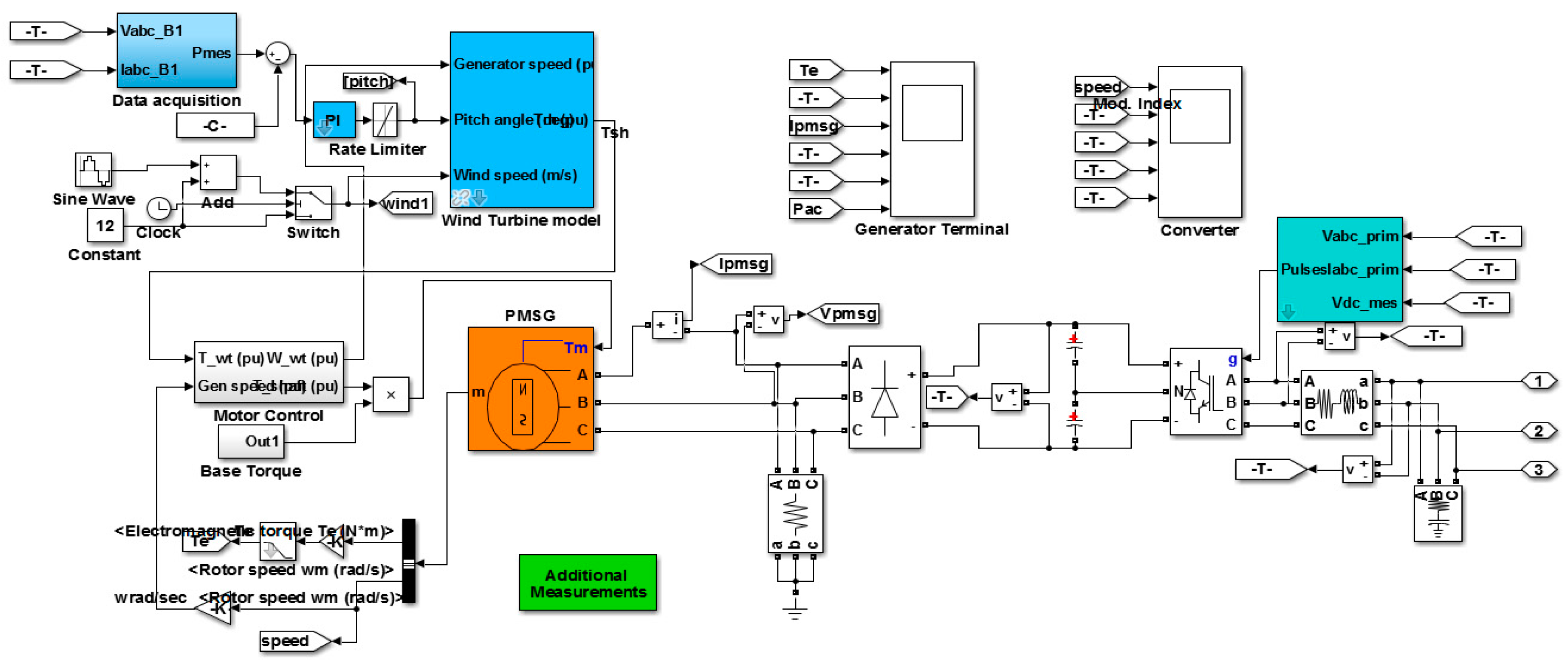
3.2. Modeling of Wind Turbine

A permanent magnet synchronous generator (PMSG) was used to generate a maximum rated power of 200 kW with a two-mass drive train model for coupling the wind turbine and generator, and pitch angle control at high wind speed [39]. The model is shown in Figure 5. An average hourly variable wind speed input was incorporated based on Australian hemisphere-collected data from the Bureau of Meteorology (BoM) [38]. The mechanical power output from the wind turbine is given by Equation (4):

$$P_m=\raisebox{1ex}{$1$}\!\left/ \!\raisebox{-1ex}{$2$}\right.\rho A{C}_p{V}_w^3$$

(4)

where $\rho$ is the air density, $A$ is the sweep area of the turbine blades, $V_w$ is wind speed, and $C_p$ is the aerodynamic power coefficient.

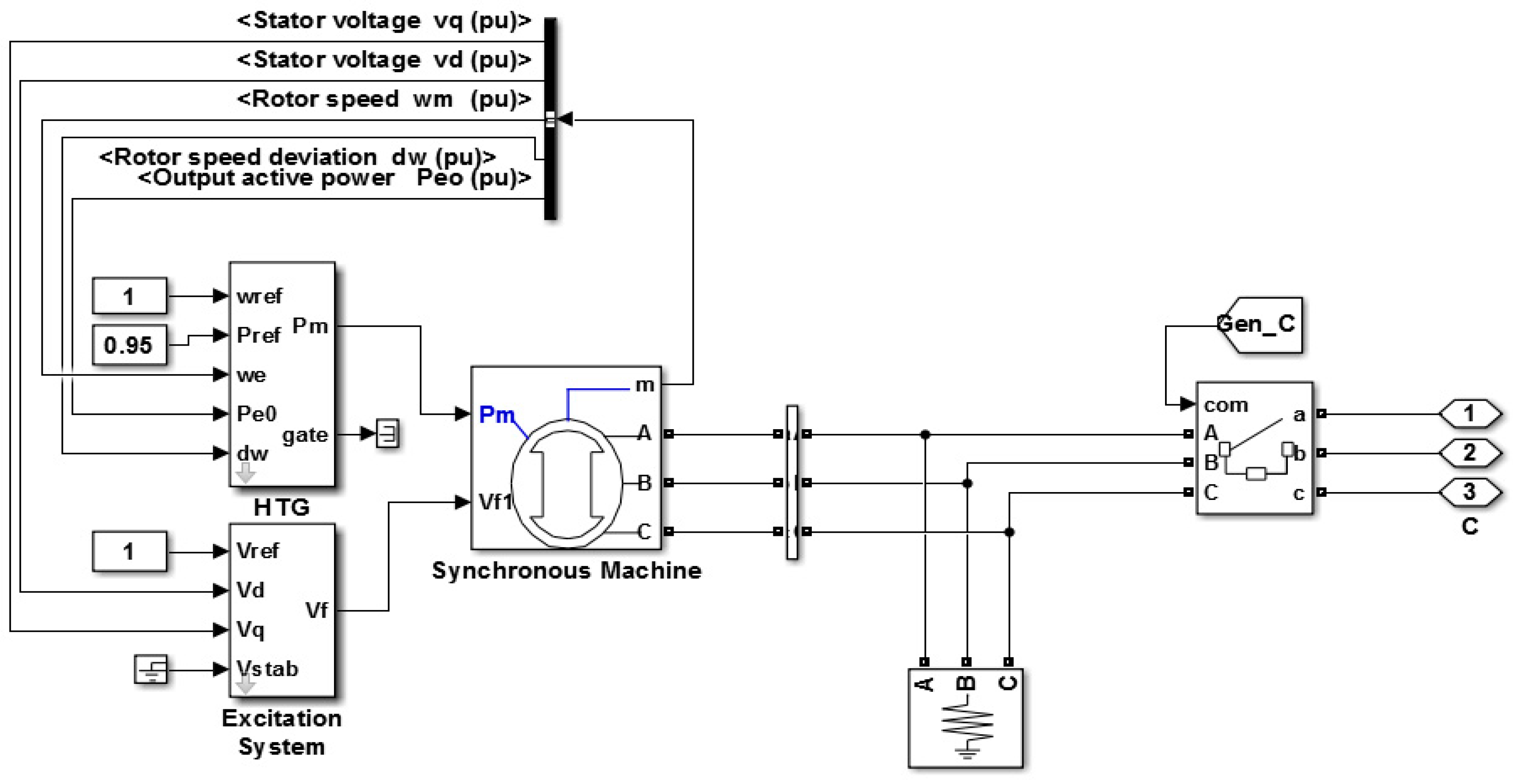
3.3. Modeling of Diesel Generator

A three-phase generator, rated 150 kW, 25 kV, and 112.5 rpm, was connected to the grid for back-up generation whenever there were any faults or load shedding detected in [40]. The generator we have modelled in MATLAB is a synchronous machine. Figure 6 shows the model of the diesel generator.

4. Selection of the Communication Medium

The communication infrastructure for advanced DSM implementation needs two different types of communication. These communications exchange data information flow between the utility control center and the participating end-users [41]. Type-1 is the communications among the sensors, devices, and the domestic appliances to the smart meter or the smart gateway, which is the main brain of the whole system that collects necessary data from the connected sensors and sends it to the utility control center. Type-2 is the communication platform between the users’ smart meters and the utility center, which can be further divided into two types: point-to-point, and mesh networks [17]. The point-to-point communication platform is more like an open access network. It communicates with smart meters by authorized entities, using a third party telecommunication network through passwords. In general, it is used in a specific geographic region where smart meters are given to a limited number of individuals supplied by different service providers.

The mesh network is a communication platform among a group of smart meters which form a meshed radio network to communicate with each other. Working as a signal repeater, each meter sends the data to the electric network access point, which transfers it to the utility control center via a coherent communication network. A mesh network platform is more flexible and efficient, as it is more cost-effective than a point-to-point network. However, network capacity is limited in the mesh network, and it is also sensitive to interference and fading [42].

The two-way communication of data information between the utility and consumers’ home appliances are mainly adopted by two communication schemes: wired, and wireless communication. These can be classified into: Home Area Network (HAN), Neighborhood Area Network (NAN), and Wide Area Network (WAN). HAN requires very low bandwidth, and is a cost-effective network platform for communication between home appliances and the gateway or smart meter. In home applications, HAN informs the consumers about the energy consumption and other profiles via a web interface or internal display. Multiple end-users situated in a specific geographic region can be directly connected to the data concentrator or substation via the HAN system. Some examples of the HAN system are ZigBee, WiFi, M-BUS, Z-wave, HomePlug, and Power Line Communication (PLC) [43]. NAN is very similar to HAN, and can also be established by ZigBee, WiFi, PLC, and so forth. For long-distance data transmission and a high bandwidth platform, the WAN system is more reliable and can be used for bi-directional communication between the data concentrator and the service utility control center. Multiple NANs can be connected to the utility control center via a WAN. The Fiber optic cable, Cellular networks, Microwave, and WiMAX are some popular WAN system platforms.

For the Type-1 communication platform between the home appliances and the smart gateway or smart meter, the network premises can be adopted with a low bandwidth, low power, and short-distance network technology. A wireless HAN system, such as ZigBee, Bluetooth, or WiFi is preferable compared to the wired networks, such as PLC or HomePlug. Comparatively less bandwidth per device/node, such as 14–100 Kbps, and a latency time of 2–15 s are required for the wireless HANs [44].

The comparison between different communication mediums was adopted from [45,46] and is shown in Figure 7. An ideal network platform should have equal performance across all three parameters: latency, coverage, and data rate (i.e., 33.3% each). The percentage of the parameters will explicate how balanced a medium is. According to the discussions and collected information, the most preferable network platform relative to other wireless HAN systems is ZigBee, since it has the most balanced and suitable features for operating domestic appliances as shown in Figure 7a. The data transmission range of ZigBee is up to 175 m with a data rate of 250 Kb/s, and it operates on OQPSK modulation [47]. ZigBee can coordinate a mesh network platform where some of the devices in that mesh can be operated in sleep mode when they are inactive, which results in less power consumption [48]. ZigBee is preferable and affordable because of its advantages with less power consumption and low complexities, as well as being a cost-effective form of wireless communication. In this study, ZigBee was considered for the HAN system for communications among the sensors and devices to the smart meter to control and monitor the home appliances.

The most common types of communication mediums between smart meters and utility are PLC, the Digital Subscriber Line (DSL), and cellular networks. PLC has been the first choice for communication between smart meters and the data concentrator in urban areas, where other solutions struggle to meet the needs of utilities [49]. It is the preferable choice because the existing infrastructure decreases the installation cost of the communications infrastructure, and PLC provides secure data transmission as shown in Figure 7b. However, PLC may be insufficient for some real-time applications requiring high bandwidths [50]. Furthermore, the PLC transmission medium is harsh and noisy. It is sensitive to the network topology, the number and type of the devices connected, and the wiring distance between transmitter and receiver. These all adversely affect the quality of the signal, making PLC technology unsuitable for data transmission [51]. DSL is a high-speed digital data transmission technology that uses the wires of the voice telephone network. The widespread availability, and low-cost and high-bandwidth data transmissions are the most important reasons for considering the DSL technology as a suitable communications candidate for smart meter communications to the utility. The DSL-based communications systems require communications cables to be installed and regularly maintained, and therefore cannot be implemented in rural areas due to the high cost of installing fixed infrastructure for low-density areas. Distance dependence, and a lack of standardization and reliability are disadvantages that make DSL technology less appealing. Existing cellular networks are good options for communication between smart meters and the utility, as well as between far nodes. Widespread and cost-effective benefits make cellular communication one of the leading communications technologies for smart grid applications. To manage healthy communications with smart meters in rural or urban areas, the wide area deployment of the cellular networks can cover almost 100% of areas. Lower cost, better coverage, lower maintenance costs, and fast installation features highlight cellular networks as the best candidate for the communications of DR applications. However, the services of cellular networks are shared by the customer market, and this may result in network congestion or decreases in network performance in emergency situations. Hence, these considerations can drive utilities to build their own private communications network. In abnormal situations, such as a wind storm, cellular network providers may not provide guaranteed service. In some cases, utilities prefer WiMAX due to proper security protocols, smooth communications, high data speeds, and an appropriate amount of bandwidth and scalability. However, WiMAX is not as widespread a technology as Fiber optic, meaning that the cost of installation will be higher in some areas [52]. Therefore, choices among the different types of communication technology can vary, and what may fit for one environment may not be suitable for another.

5. Modeling of the HEMS

The proposed HEMS consists of a smart load monitoring system and an intelligent load controller. The intelligent load controller takes load consumption decisions based on the data collected from the smart load monitoring system.

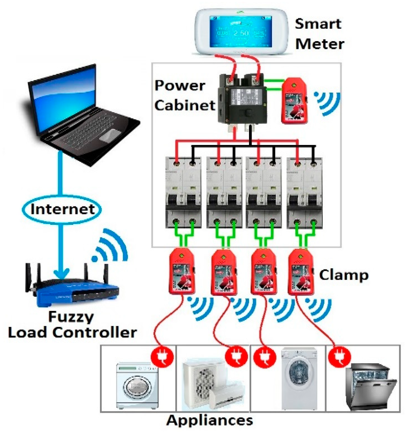
5.1. The Proposed Smart Load Monitoring System

A smart load monitoring system based on a wireless HAN network has been proposed to monitor and operate various home appliances for the HEMS to reduce the peak demand and overall energy consumption cost. This system consists of four key units: smart appliances, smart clamps, a smart meter, and a smart energy gateway, where the energy gateway is integrated with a load controller. The gateway works as a router that manages all the networking issues, allows secured wireless internet access (ZigBee), and operates real-time power management by receiving data from the smart clamps and smart appliances. Consumers can access their energy consumption information through the gateway and are able to set their consumption preferences remotely throughout the day with respect to the electricity price. Smart clamps are deployed in the power cabinet to provide metering of the entire home energy usage. The smart appliances coordinate and measure the consumption of appliances, which can be individually operated in active/inactive states and can be shifted automatically, and is remotely based on load controller decisions. Moreover, real-time information on the amount of energy consumption can be provided to the consumers on the panel of the smart meter, in which alarms will be generated and appear on the panel if there is any abnormality detected on the grid. The overall architecture of the proposed HEMS is shown in Figure 8.

The smart meter collects various bits of information, such as electricity price, weather conditions (temperature), the utility load control signal, connection point voltage profile, and the like, and sends this information at specific intervals (e.g., every 15 min) to the gateway of the load controller. The load controller uses this information for load consumption and load-shifting decisions.

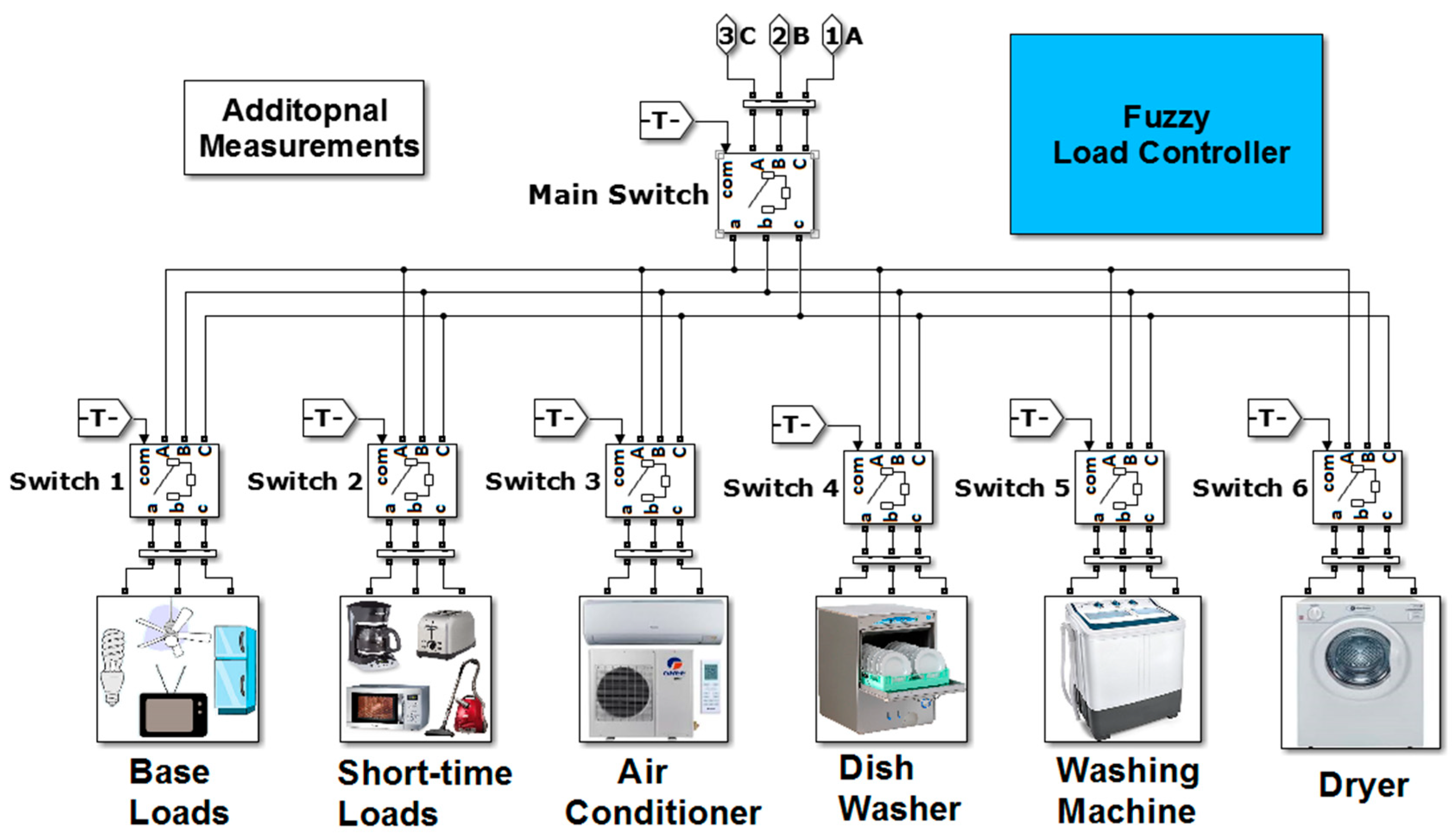
5.2. Intelligent Load Controller

Manual device control is unattractive to residents and inefficient for managing loads when the cost of generation is high, or network condition is jeopardized. The proposed load controller can take automatic decisions on behalf of consumers to consume electricity in cost-effective and efficient ways while helping the utility to maintain a balance between generation and demand. However, lack of intelligence in the load-controlling system may create more complexity in scheduling multiple devices and may also violate consumer comfort levels [53] as simplicity, cost reduction, and comfort are the prime needs that a consumer should get from adopting a HEMS. To this aim, this study developed an intelligent decision-supporting load controller for a HEMS based on a fuzzy logic algorithm, which can help consumers to save energy costs while also satisfying their comfort levels and assisting the utility to manage their network voltage during peak demand and high RES (renewable energy source) generation periods. The fuzzy logic-based load controller considers multiple variables as an input for the load consumption decision, namely grid price signals, outdoor temperature, room temperature, available renewable energy generation, total consumption, load control signal, and so forth, which will be collected through a smart monitoring system (as discussed in the previous section).

The load controller is designed in such a way that when the consumers increase their consumption during peak hours, it shifts the non-priority loads (such as the washing machine, dishwasher, etc.) to the off-peak hours and only allows the priority loads (AC, room heater, etc.) to operate to maintain consumer comfort.

Table 1. Load categories for load controller.

Base Loads	Schedulable/Non-Priority Loads
Light	Washing machine
Fan	Dishwasher
TV	Clothes dryer
Computer	Short-time loads
Refrigerator	Coffee maker
Priority loads	Toaster
AC	Vacuum cleaner
Room heater	Micro-oven

shows the defined load categories for the fuzzy load controller.

Consumers can pre-set the deadline of the operational time of each non-priority load. The utility can send load control signals to the HEMS for managing the network. The controller also keeps load consumption within a certain limit (in this example, 2.5 kW maximum) which means the load consumption will not exceed the limit during the high peak hours. However, it will allow the consumer to exceed the limit only if the load consumption time is less 16 min. For instance, if a consumer is currently operating 2.5 kW of total load during a peak period and turns the coffee maker and microwave on with time settings less than 16 min, as the smart meter sends information at 15-min intervals, the load controller will allow such higher consumption for a short period of time. Hence, the load controller of the HEMS takes optimal decisions for load consumption and scheduling based on minimization of comfort level violation, energy costs, and network violation. If the consumer has onsite generation, the HEMS load controller will always consume energy from the available renewable energy generator (such as the wind turbine, PV, batteries, etc.) first. If there is any surplus energy from the renewable resources, the batteries will be charged (if available) and the remaining energy will be kept for peak-period usage or sold back to the utility grid. Figure 9 shows the developed Simulink (MATLAB) model of the proposed load control system which is connected with the home electric appliances through controllable switches.

The next section provides detailed modeling of the fuzzy load controller.

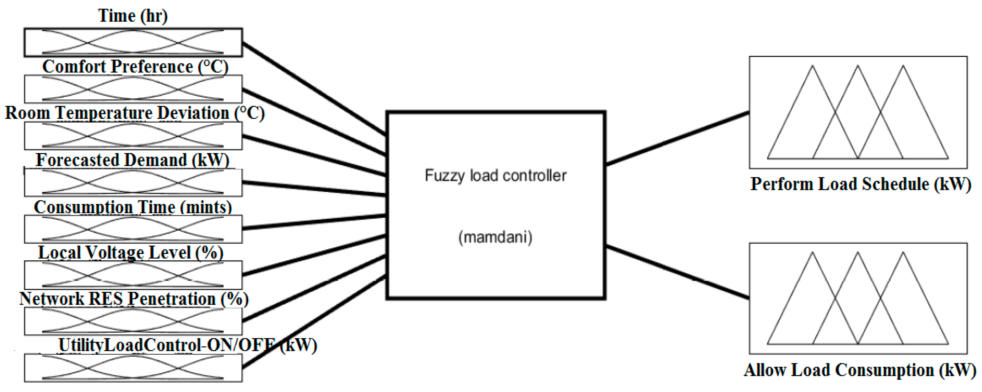
5.3. Fuzzy Load Controller

A fuzzy logic algorithm works with a well-defined set of rules. It can handle problems with imprecise and incomplete data and can also model nonlinear functions of arbitrary complexity. The benefit of using fuzzy logic is its interpretability and simplicity. To develop the load controller using a fuzzy logic algorithm, the following parameters are defined:

• Input and Output of the fuzzy load controller
• Fuzzy Membership Functions
• Fuzzy Rules

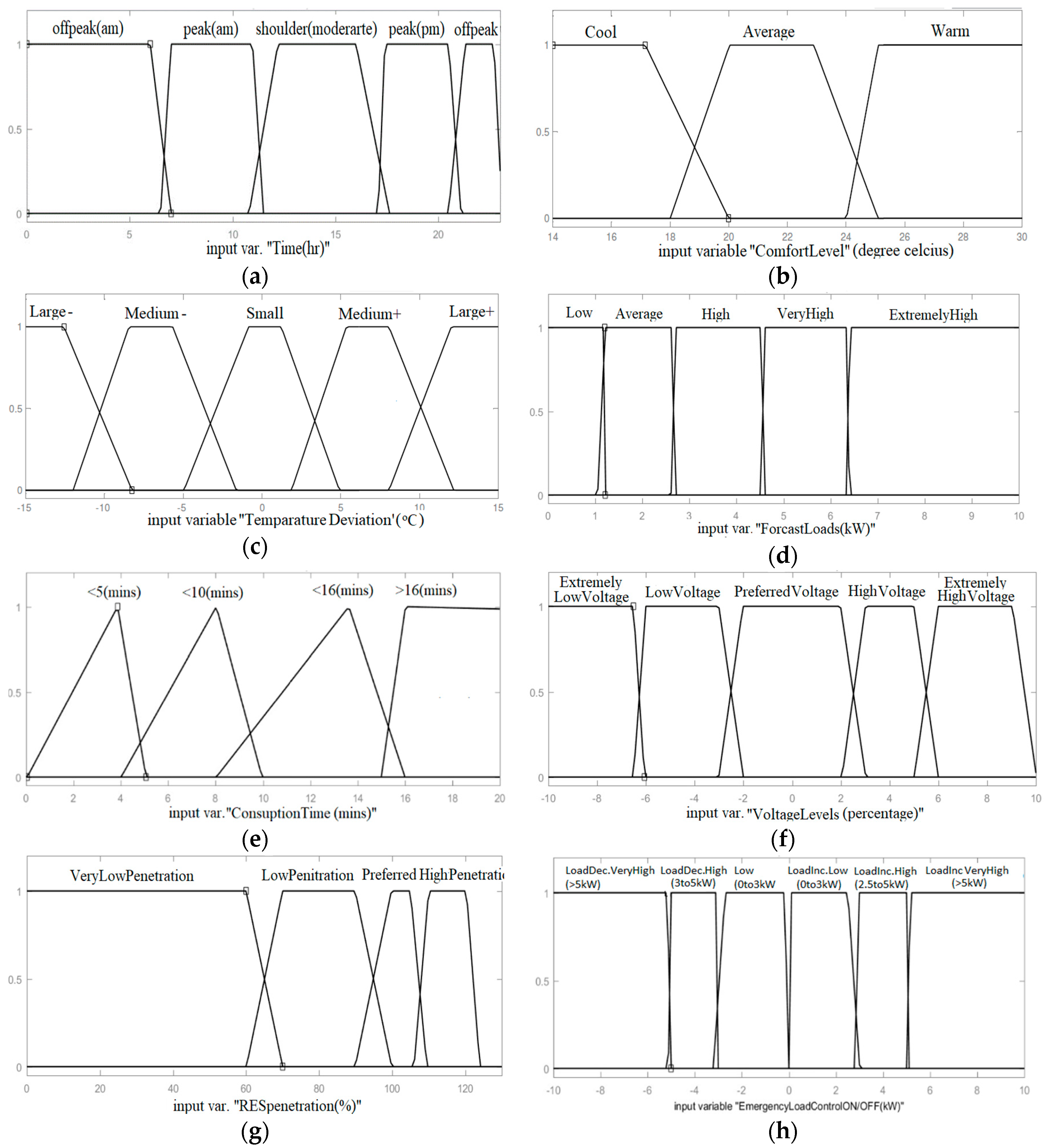
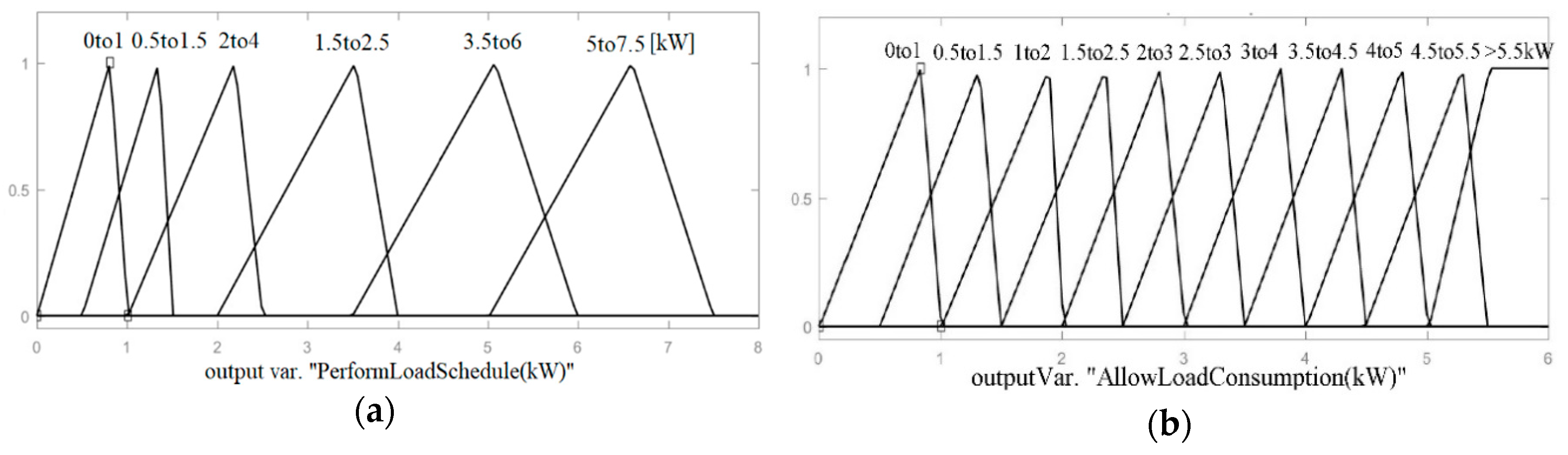
5.3.1. Input and Output of the Fuzzy Load Controller

The load controller has 8 input and 2 output variables, as shown in Figure 10. The input variables are:

Input1—Time (Dynamic pricing signals): A day is divided into five periods of peak (am), peak (pm), off-peak (am), off-peak (pm), and shoulder (moderate), which are included in fuzzy membership function as a trapezoidal type.

Input2—Comfort preference: The desired room temperature level (°C) for priority loads (i.e., AC, room heater) set by the consumers at which they feel comfortable.

Input3—Room temperature deviation: Room temperature deviation from the consumer’s comfort-level temperature.

Input4—Forecasted demand: The load forecast in this study is considered based on the user’s predefined consumption preference setting on a daily basis. The load controller then uses the users’ predefined consumption preferences to estimate the total load demand at each 15-min interval.

Input5—Consumption time: The consumption time (in minutes) of each load.

Input6—Local voltage level: The supplied voltage level at the point of connection.

Input7—Network RES penetration: The RES penetration (%) at the main transformer is calculated by Equation (5). The load controller uses this information to balance out the generation and demand.

$$RESpenetration(\%)=\frac{totalRESgeneration}{totalloaddemand}\times 100$$

(5)

Input8—Utility load control (DLC signals)-ON/OFF: Utility may send load ON/OFF signals to the load controller to maintain network reliability.

Output1—Perform load scheduling: The total amount of loads in kW that are shifted to an off-peak period.

Output2—Allow load consumption: The total amount of loads in kW that the controller allows to operate in the current period of time.

The controller takes the crisp or real input values from the smart monitoring system, fuzzifies them, and assigns a fuzzified control signal to provide control over the loads based on the assigned rules and membership functions. The control signal is then converted into two output crisp signals through a defuzzification process.

5.3.2. Fuzzy Membership Functions

The input and output variables of the fuzzy load controller are constructed with fuzzy membership functions to define the linguistic rules that govern the input and output relationships. The membership functions of input variables are more compatible with a trapezoidal type for the load controller. In contrast, the output variables are defined with a triangular type because of the sharp constraints on those variables. The values of membership functions are defined based on realistic load profiles of typical home appliances (as shown in Section 6.1). Figure 11a–h show the inputs membership functions of the fuzzy load controller. Figure 11a defines the time of day, which has been divided into five sections: peak (am), peak (pm), off-peak (am), off-peak (pm), and shoulder (moderate). Figure 11b shows the desired room-temperature level (°C) of the customer’s comfort preferences, which is divided into Cool, Average, and Warm. Figure 11c shows room-temperature deviation from the range of consumer comfort-level temperatures from −15 to +15, such as: Negative Large, Negative Medium, Small (which ranges from −5 to +5), Positive Medium, and Positive Large. Figure 11d portrays the forecasted load based on customers’ predefined consumption, which is divided into Low, Average, Medium, High, and Extremely High. Figure 11 delineates the consumption time of loads, which ranges from 0 to 20 min. Figure 11f shows the input voltage level of the grid, which has been divided into five sections. Figure 11g illustrates the total RES penetration of the grid, and ranges from 0% to 120%. Figure 11h describes an emergency load control (ON/OFF) which operates based on the load-decrement control signal from the utility. Figure 12a,b show the output membership functions of the fuzzy load controller.

5.3.3. Fuzzy Rules

The load controller operates based on predefined fuzzy rules. The number of rules framed depends on the number of membership functions considered in the input and output blocks. The more rules there are, the more precise the load controller output will be. This study developed 50 rules; 8 of them are listed below as examples.

(1) If (Time is peak (pm)) and (Comfort preference (°C) is Cool) and (Room Temperature Deviation (°C) is Large+) and (Forecasted Load (kW) is Very High) and (Consumption Time is >16 (mints)) and (Voltage Level (%) is Low Voltage) and (RES penetration (%) is Very Low Penetration) then (Perform Load Schedule (kW) is 3.5 to 6 (kW)) and (Allow Load Consumption (kW) is 1 to 2 (kW)).

(2) If (Time is peak (pm)) and (Comfort preference (°C) is Cool) and (Room Temperature Deviation (°C) is Large+) and (Forecasted Load (kW) is Extremely High) and (Consumption Time is >16 (mints)) and (Voltage Level (%) is Low Voltage) and (RES penetration (%) is Very Low Penetration) then (Perform Load Schedule (kW) is 5 to 7.5 (kW)) and (Allow Load Consumption (kW) is 1 to 2 (kW)).

(3) If (Time is shoulder (moderate)) and (Comfort Preference (°C) is Cool) and (Room Temperature Deviation (°C) is Large+) and (Forecasted Load (kW) is Very High) and (Consumption Time is >16 (mints)) and (Voltage Level (%) is Preferred Voltage) and (RES penetration (%) is Low Penetration) then (Perform Load Schedule (kW) is 1.5 to 2.5 (kW)) and (Allow Load Consumption (kW) is 3 to 4 (kW)).

(4) If (Time is off-peak (am)) and (Comfort Preference (°C) is Average) and (Room Temperature Deviation (°C) is Small) and (Forecasted Load (kW) is Very High) and (Consumption Time is >16 (mints)) and (Voltage Levels (%) is High Voltage) and (RES penetration (%) is High Penetration) then (Allow Load Consumption (kW) is 4.5 to 5.5 (kW)).

(5) If (Time is peak (pm)) and (Comfort Preference (°C) is Cool) and (Room Temperature Deviation (°C) is Large+) and (Forecasted Load (kW) is Very High) and (Consumption Time is >16 (mints)) and (Voltage Levels (%) is Extremely Low Voltage) and (RES penetration (%) is Very Low Penetration) and (Utility Load Control ON/OFF (kW) is Load Dec. High (3 to −5 kW)) then (Perform Load Schedule (kW) is 3.5 to 6 (kW)) and (Allow Load Consumption (kW) is 0.5 to 1.5 (kW)).

(6) If (Time is shoulder (moderate)) and (Forecasted Load (kW) is Extremely High) and (Consumption Time is >16 (mints)) and (Voltage Level (%) is Extremely High Voltage) and (RES penetration (%) is High Penetration) then (Allow Load Consumption (kW) is >5 (kW)).

(7) If (Time is peak (am)) and (Comfort Preference (°C) is Cool) and (Room Temperature Deviation (°C) is Medium+) and (Forecasted Demand (kW) is Extremely High) and (Consumption Time (mints) is <10 (mints)) and (Local Voltage Level (%) is Preferred Voltage) and (Network RES penetration (%) is Preferred Penetration) then (Allow Load Consumption (kW) is >5 (kW)).

(8) If (Time is peak (am)) and (Comfort Preference (°C) is Cool) and (Room Temperature Deviation (°C) is Small) and (Forecasted Demand (kW) is Very High) and (Consumption Time (mints) is <10 (mints)) and (Local Voltage Level (%) is Low Voltage) and (Network RES penetration (%) is Low Penetration) then (Perform Load Schedule (kW) is 0 to 1 (kW)) and (Allow Load Consumption (kW) is 4.5 to 5.5 (kW)).

A case study was conducted to analyze the benefits and performance of the proposed HEMS within a microgrid environment, as presented in the next section.

6. Case Study Analysis

To identify the actual benefits of the proposed HEMS and perform a realistic cost saving analysis, this study deployed a smart load monitoring system in a typical three-bedroom house in the suburb of Ferndale in Perth, Australia. The power consumption data was collected by a smart load-measuring device on a typical summer day of December. The collected daily load profiles of each electric appliance from the house were then implemented on a MATLAB simulation model of the load controller (see Figure 8) for evaluating the performance of the load controller and calculating a realistic cost saving analysis in the microgrid environment.

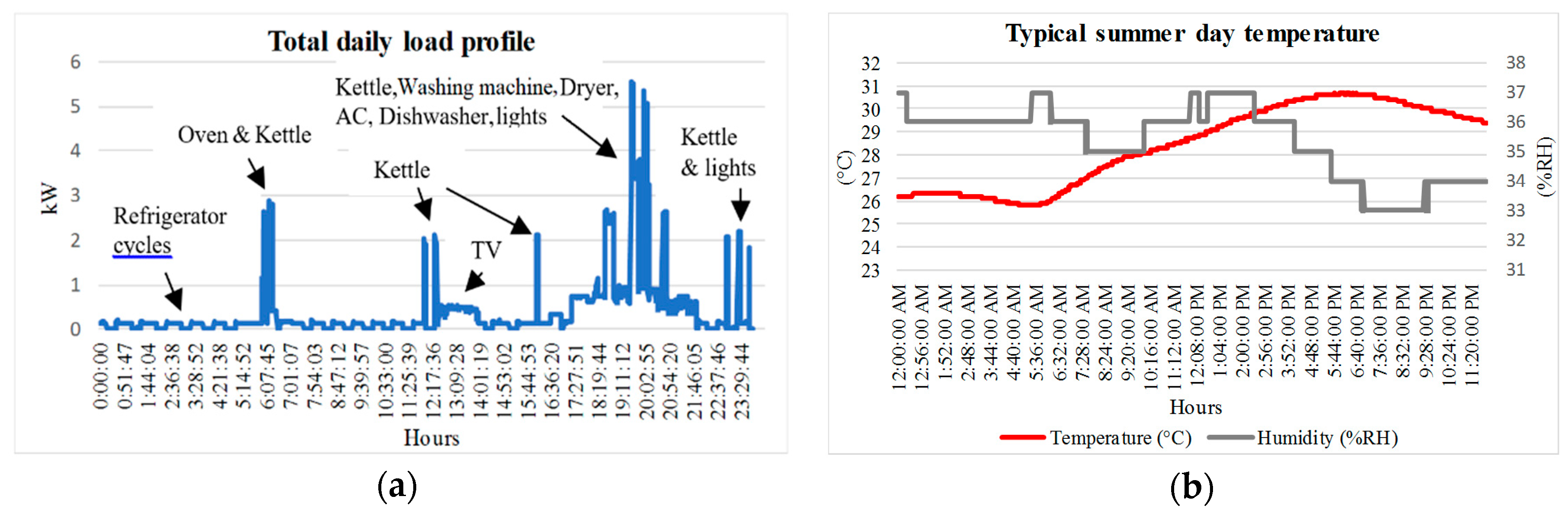
6.1. Load Profiles of a Typical House

Figure 13a illustrates the typical daily load profile of a household during a summer day obtained from the smart monitoring system. It shows that the peak demand occurs during the evening period due to usage of all major loads in this period. Figure 13b shows the room temperature and humidity on that summer day, which has been collected by a room sensor. The power consumption profiles of five major appliances are shown in Figure 14. It can be observed that the consumption characteristics of all these major appliances are that they have cyclic patterns, and that they consume standby power losses.

6.2. Energy Cost Saving Analysis with HEMS

According to the consumer load profiles, weather conditions, electricity price, and utility load control signals obtained from the smart monitoring system and the fuzzy defined rules, the fuzzy load controller optimizes the load operation and schedules the non-priority loads.

Table 2. Optimized results from the fuzzy load controller.

Input Conditions									Optimized Outputs
Fuzzy Rules	Time	Comfort Preference (°C)	Temperature Deviation (°C)	Forecasted Load (KW)	Consumption Time (mints)	Local Voltage Level (%)	Network RES Penetration (%)	Load Control (kW)	Perform Load Schedule (KW)	Allow Load Consumption (KW)
1	peak (pm)	16	14	5.4	16>	−4%	60%	0	3.74	1.89
2	peak (pm)	17	13	8.3	16>	−4%	60%	0	6.37	1.64
3	shoulder	17	12	5.4	16>	−1.60%	80%	0	1.9	3.6
4	off.pk (am)	22	1.2	4.8	16>	+4%	120%	0	0	5.1
5	peak (pm)	16.5	14.5	5.4	16>	−7%	50%	Dec. = 4.0	4.86	1.11
6	shoulder	non	non	6.6	16>	+8%	115%	0	0	7.3
7	peak (am)	17	8	6.5	<10	+0.50%	104	0	0	7.3
8	peak (am)	17	8	5.5	<10	−3%	88%	0	0.61	5.1

shows the optimized load operations using the fuzzy load controller based on the input conditions. It can be seen that in fuzzy rule 1, when the load consumption occurs in the evening peak period and the consumer’s preferred comfort level for room temperature is 16 °C (which is a 14 °C deviation from the current room temperature), the forecasted load is very high (5.4 kW) and is made up of the current available loads to be operated {i.e., AC (0.6 kW) + W.mch (1.9 kW) + D.wash (1.8 kW) + base load (1.1 kW) = 5.4 kW} and the consumption time of these loads is more than 16 min. The current voltage level at the connection point is low (4% less than the standard voltage) and the total RES penetration at the transformer secondary side is very low (60%), which means that if generation is 200 kW and load demand is 333 kW, the RES penetration is 60% (200*100/333). As there is no load control signal from the utility, then the optimized outputs of the load controller are: perform load schedule 3.74 kW {which is equivalent to W.mch (1.9 kW) + D.wash (1.8 kW) = 3.7 kW} and allowable load consumption is 1.89 kW {equivalent to AC (0.6 kW) + base load (1.1 kW) = 1.7 kW}. This means that fuzzy rule 1 allows the consumer to maintain their comfort level temperature by operating the AC during the hot summer evening peak period, as well as operating the basic loads while trying to improve the local voltage level and balance the generation and demand in the microgrid, as well as to reduce the energy cost during this peak period by shifting non-priority loads to off-peak periods. Rule 2 shows similar conditions as to rule 1. Unlike rules 1 and 2, rule 3 reduces the high load schedule value, as the current local voltage condition (−1.6%) is in the preferred voltage level range (within ±3% of the nominal voltage), RES penetration is not too low (80%), and consumption occurs in a shoulder period (the shoulder period price is less than the peak period price). By contrast, in rule 4, no load scheduling is being performed due to being in an off-peak consumption period (off-peak period has minimum $/kWh price), with a high voltage level and high RES penetration. In rule 5, the load controller schedules all loads, including AC operation, except the basic loads (1.1 kW) due to a load decrement control signal from the utility (4 kW), extreme low voltage, and low network RES penetration conditions. Rule 6 allows no scheduling of loads and operates all forecasted loads due to the high local voltage level, high RES penetration level, and shoulder period consumption. Rule 7 allows for the extremely high forecasted loads (6.6 kW) to operate even in a peak period without any load scheduling because the load consumption time is less than 10 min {e.g., the forecasted load (6.5 kW) = AC (0.6 kW) + base load (1.1 kW) + short-term load (3 kW) + D.wash (1.8 kW)}. However, for rule 8, about 0.61 kW of the load (which is equivalent to AC consumption) is scheduled, even though the consumption time is less than 10 min, due to the low local voltage level and low network RES penetration.

Table 3. Energy cost savings analysis.

Load Type	Peak Shaving Capacity (kW)	Shiftable Energy (kWh)	Standby Energy Loss (kWh)/day	Total Energy Cost without HEMS ($/day)	Total Energy Cost with HEMS ($/day)	Cost Saving (%/day)
Base loads	N/A	N/A	0.02	$3.49 (total daily energy 9.40 kWh)	$2.50 (total daily energy 9.16 kWh)	28.4% (total daily energy saving 3%)
AC	N/A	N/A	0.14
W.mach	1.9	0.64	0.012
D.wash	1.8	0.57	0.034
Dryer	3.0	1.38	0.035

shows the potential peak demand shaving capacity, energy shifting capacity, and standby energy loss of the appliances of a typical house which are obtained from a smart monitoring system installed in the house. It also presents the calculated daily energy costs with HEMS and without HEMS. The cost comparisons of the daily load profile are performed by shifting the energy usages of non-priority loads from peak periods to the off-peak period. The standby energy loss is also included in the cost analysis. With the HEMS there will be no standby energy loss. The per-unit cost ($/kWh) of electricity for off-peak ($0.14/kWh), shoulder ($0.26/kWh), and peak ($0.50/kWh) periods are taken from [19], which are based on a smart home (SM1) tariff plan in Australia. Table 3 shows that the total daily energy cost without HEMS is $3.49 (for a total of 9.40 kWh of energy consumption), whereas it becomes $2.50 (for a total of 9.16 kWh of energy consumption) with the HEMS, which amounts to energy cost savings of about 28.4% per day.

Based on the results in Table 2 and Table 3, it can be observed that the proposed HEMS reduces excessive consumption when the energy consumption prices are very high or when the network voltage and RES penetration are in critical conditions, while maintaining consumer comfort levels and providing energy cost savings.

7. Microgrid Analysis with HEMS

In this study, the microgrid system, based on solar PV, a wind turbine, and a diesel generator, was designed so as to supply 100 houses in a remote region in Western Australia. The estimated total power generation was 500 kW, of which 150 kW was supplied from the solar PV farm, 200 kW from the wind turbine, and the remaining 150 kW supplied from the diesel generator.

Hourly solar radiation and wind speed data was calculated on a typical day in December based on the data available at the Bureau of Meteorology (BoM), Australia, at a location of Perth, Australia. Figure 15 shows the hourly solar radiation and wind speed used for simulation.

The power produced by the solar panels, the wind turbine, and the diesel generator are shown in Figure 16 on an hourly basis, which provides a total of 500 kW generation by the microgrid on a typical day.

7.1. Residential Loads and Demand Analysis in Microgrid

In this study, it has been considered that the stand-alone microgrid system was supplying 100 houses in a remote region in Western Australia with an estimated generation capacity of 500 kW. To evaluate the effectiveness of the proposed HEMS, the load profiles of 100 consumers have been clustered into four different consumer groups where load consumptions were varied during different times of day, as each house has its unique pattern of load consumption. Figure 17a–d show the load profiles of one typical house from each of the four groups that have been considered for this study. Figure 18 represents the total energy demand by 100 houses in the microgrid during a typical day.

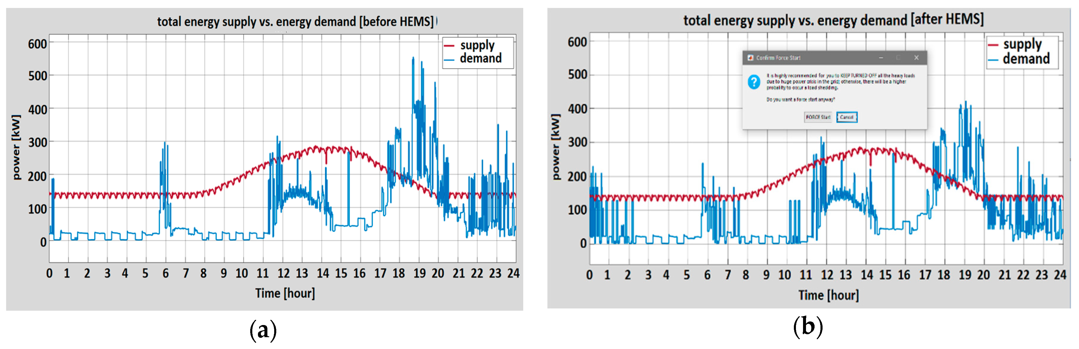
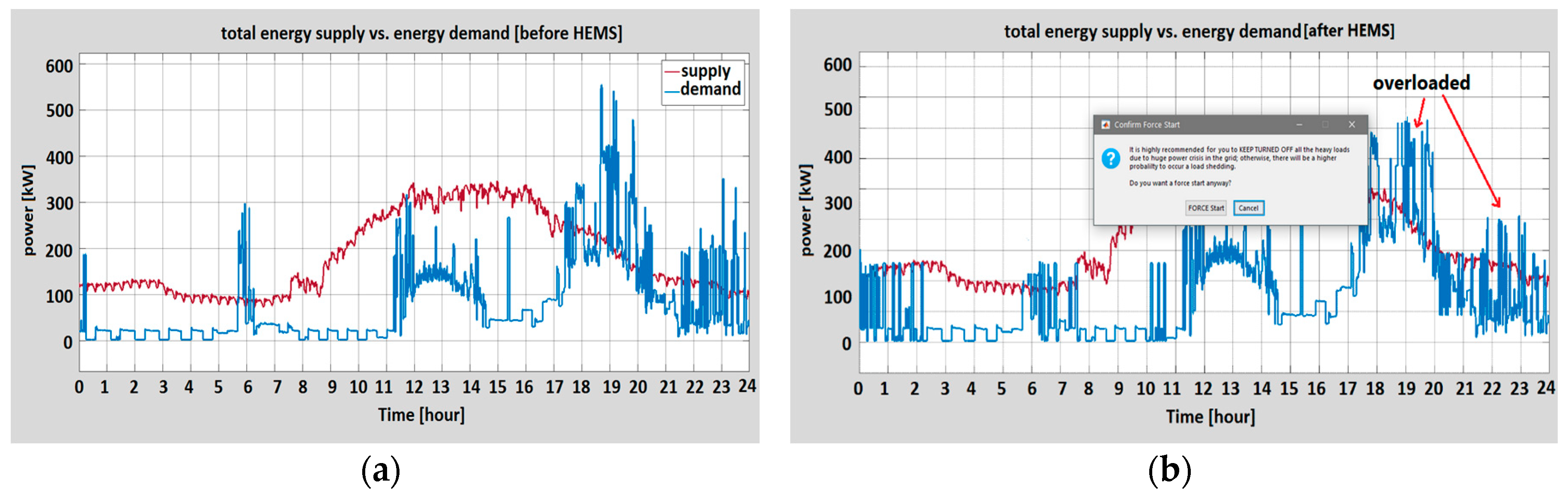
7.2. Demand Response Opportunity in Microgrid

To investigate the actual benefits of the proposed HEMS and perform a realistic cost-saving analysis for the total microgrid system, the smart load monitoring and controlling system was deployed in each house. The collected daily load profiles of each electric appliance from the house are implemented in the MATLAB simulation model of the fuzzy-based load controller (see Figure 10) considering 100 houses, which helped evaluate the performance of the load controller and to calculate total realistic energy savings in the whole microgrid.

Furthermore, to scrutinize more realistic results and feedback from the HEMS on how the system handles different critical or worst-case scenarios, the system was simulated in four different scenarios with respect to availability of the individual power sources, as follows:

• Scenario A: only the solar farm and the diesel generator are supplying the residential loads.
• Scenario B: the solar farm and wind farm are active.
• Scenario C: the wind farm and the diesel generator are available, but the diesel generator is partially ON only in the high demand period.
• Scenario D: all the sources are simultaneously active, except for the diesel generator, which only turns ON when it is needed.

The studied scenarios only focused on the long-term variability of RES-based generation and load demand. The diesel generator was used as a back-up resource to ensure that the reliability of the system was caused by high variability of RES-based generation and load demand in a short period of time. The diesel generation had a very fast response, with a load pick-up capability of less than 1 min. Moreover, the developed HEMS had an ability to respond to the load control signal from utility (i.e., direct load control DR program) to support the high variability of RES-based generation (as mentioned in fuzzy rule 5 in Section 5.3.3).

As shown in Figure 19, it is noticeable from the simulation results that the total energy demand of the residential loads surpasses the total generated power in Scenario A, and that peak demand occurs for a certain period which has been plotted in Figure 19a,b, keeping the fuzzy load controller inactive and active, respectively. There are several critical conditions that are noticeable in the grid when the energy demand is very high and the RES penetration is very low. It can be seen that the RES penetration in the night time is extremely low, since solar panels are unable to supply any electricity; and in the evening period, when the room temperature is high (see Figure 13b), an enormous demand for air conditioners causes an extreme peak in the grid. In Figure 19b, with an optimized HEMS system, it can be seen that there is still a deficiency in the peak period, although it is reduced by shifting corresponding loads and the turning off of various loads, according to the fuzzy rules. Another DG can be added to the system to meet this peak demand.

To ensure that consumers’ comfort levels are maintained, the major appliances, including the AC and the refrigerator, are not interfered with, except that in the case of emergency, the AC compressor can be switched off by the HEMS for a few minutes. However, even though there would be a higher probability of load shedding, there will still be an optional Force Start condition in order to keep the consumers’ comfort uninterrupted and allow their independency in regard to controlling their own appliances. An additional option will also appear on the control screen, as shown in Figure 20.

During peak demand, the utility can send a direct load control signal to the HEMS. The HEMS then optimizes the operation of the appliances based on consumers’ preferences and the load control signals from the utility. Figure 21, Figure 22 and Figure 23 delineate the overall scenarios of the DR strategy for Scenario B, C, and D, respectively, where the fuzzy HEMS controller senses the crossed-off situation and, according to the fuzzy rules, it immediately turns OFF the corresponding loads except for the base-preferred loads, and shifts them to the off-peak period. In addition, according to the forecasted load, the diesel generator can be activated to perform as a back-up generation source when needed.

In Scenario C and D, the diesel generator is inactive during the high RES penetration and low-demand periods in the grid, which saves both fuel costs and unnecessary power loss.

From the acquired results of the simulations, it is clearly noticeable that the proposed HEMS is performing effectively according to the designed demand response framework in the various scenarios, as well as during critical conditions in the grid. It also mitigates excessive consumption when the energy consumption prices are very high, or when the network voltage and RES penetration are in extreme conditions. Moreover, it maintains consumers’ comfort levels and provides energy cost savings.

Table 4. Feedback of HEMS system under various grid conditions.

Grid Condition (Scenario)	Total RES Penetration (kW)	Duration of Demand Surpassing (h)	Average Load Consumption Allowance	Load Shifting Frequency	Consumers’ Comfort Level	Diesel Gen. Fuel Consumption
Scenario A	150~300	>4.5	Very Low	Very High	Interrupted (Alarm Generated)	High
Scenario B	200~350	>4	Low	High	Interrupted (Alarm Generated)	N/A
Scenario C	200~350	>3	Medium	Medium	Not Interrupted	Medium
Scenario D (All sources available)	350~500	>2.5	More	Low	Not Interrupted	Low

compares the overall outcomes, as well as the pros and cons after the HEMS system has been deployed in the microgrid under various grid conditions. The automated load controller successfully manages to handle all the situations; however, it interrupts consumers’ comfort levels only under critical conditions in the grid when RES penetration is extremely low. For instance, as it was considered that the 100 houses took part in the DR platform, for the appliances that have high DR potential (dishwasher, washing machine, and dryer) during peak periods, the total possible peak shaving capacity, energy-saving potential, and the standby loss for all 100 houses in the microgrid can be calculated as follows:

Calculating the total maximum possible peak shaving capacity (kW):

$$100*\left(1.9\mathrm{kW}+1.8\mathrm{kW}+3\mathrm{kW}\right)=670\mathrm{kW}\left(or,0.67\mathrm{MW}\right)$$

Also, calculating the maximum possible shiftable energy for 100 houses (kWh):

$$100*\left(0.64\mathrm{kWh}+0.57\mathrm{kWh}+1.38\mathrm{kWh}\right)=259\mathrm{kWh}$$

Consequently, calculating the maximum standby power loss of all the household appliances, including all the potential loads except the base loads (kWh/day):

$$100*21\mathrm{h}*\left(0.14+0.012+0.034+0.035\right)=22.1\mathrm{kWh}$$

where 21 h represents the estimated time for the appliances to remain on standby in a day.

Furthermore, calculating the energy cost of all 100 houses with and without HEMS ($/day):

$$\begin{gathered} \mathrm{Without}\mathrm{HEMS}:100*\left(\$3.49\right)=\$349/\mathrm{day}\left(\mathrm{total}\mathrm{daily}\mathrm{energy}949\mathrm{kWh}\right) \\ \mathrm{With}\mathrm{HEMS}:100*\left(\$2.50\right)=\$250/\mathrm{day}\left(\mathrm{total}\mathrm{daily}\mathrm{energy}916\mathrm{kWh}\right) \end{gathered}$$

The daily total power loss from the standby appliances and grid inefficiency due to peak demand is notable, and it would be more crucial if all the houses of a particular city were considered. It provokes enormous proliferation of electricity costs of a consumers’ monthly energy bill. This phenomenon supports the necessity of practicing demand response in future smart grid systems.

8. Conclusions

A comprehensive demand side management framework incorporating a smart fuzzy load controller and demand response in a microgrid environment has been proposed in this study to mitigate peak demand, power loss, and grid inefficiency, as well as to reduce energy costs. A smart load monitoring system takes information from appliances, and a fuzzy load controller uses this information for load consumption and load-shifting decisions. The performance of the load controller has been evaluated through a case study, and a realistic cost-saving analysis has been performed. This framework explicitly defines the effectiveness of using a fuzzy logic-based smart load controller in a smart grid framework equipped with various operational, matching, and optimization techniques. The case study analysis demonstrates that the framework helps in determining potential DR opportunities, standby power consumption, total power consumption due to standby loss, and possible peak clipping capacity.

The model can be further improved by introducing more RESs and analyzing the behavior of the system according to the stochastic actions of the intermittent resources. To improve the decision-making process of the HEMS, the generation forecast can be integrated into the HEMS. For future research, this study will further investigate the HEMS operations with an integrated RES-based generation forecast.

References

1. Yoldaş, Y.; Önen, A.; Muyeen, S.M.; Vasilakos, A.V.; Alan, İ. Enhancing smart grid with microgrids: Challenges and opportunities. Renew. Sustain. Energy Rev. 2017, 72, 205–214. [Google Scholar] [CrossRef]
2. Shafiullah, G.M. Hybrid renewable energy integration (HREI) system for subtropical climate in Central Queensland, Australia. Renew. Energy 2016, 96, 1034–1053. [Google Scholar] [CrossRef]
3. Lee, E.K.; Shi, W.; Gadh, R.; Kim, W. Design and Implementation of a Microgrid Energy Management System. Sustainability 2016, 8, 1143. [Google Scholar] [CrossRef]
4. Elsied, M.; Oukaour, A.; Gualous, H.; Brutto, O.A.L. Optimal economic and environment operation of micro-grid power systems. Energy Convers. Manag. 2016, 122, 182–194. [Google Scholar] [CrossRef]
5. Rahman, M.M.; Arefi, A.; Shafiullah, G.M.; Hettiwatte, S. Penetration maximisation of residential rooftop photovoltaic using demand response. In Proceedings of the 2016 International Conference on Smart Green Technology in Electrical and Information Systems (ICSGTEIS), Bali, Indonesia, 6–8 October 2016; pp. 21–26. [Google Scholar]
6. Broeer, T. Analysis of Smart Grid and Demand Response Technologies for Renewable Energy Integration: Operational and Environmental Challenges. Ph.D. Thesis, University of Victoria, Victoria, BC, Canada, 2015. [Google Scholar]
7. Rahman, M.M.; Arefi, A.; Shafiullah, G.M.; Hettiwatte, S. A new approach to voltage management in unbalanced low voltage networks using demand response and OLTC considering consumer preference. Int. J. Electr. Power Energy Syst. 2018, 99, 11–27. [Google Scholar] [CrossRef]
8. Aghajani, G.R.; Shayanfar, H.A.; Shayeghi, H. Presenting a multi-objective generation scheduling model for pricing demand response rate in micro-grid energy management. Energy Convers. Manag. 2015, 106, 308–321. [Google Scholar] [CrossRef]
9. Safamehr, H.; Rahimi-Kian, A. A cost-efficient and reliable energy management of a micro-grid using intelligent demand-response program. Energy 2015, 91, 283–293. [Google Scholar] [CrossRef]
10. Bruni, G.; Cordiner, S.; Mulone, V.; Sinisi, V.; Spagnolo, F. Energy management in a domestic microgrid by means of model predictive controllers. Energy 2016, 108, 119–131. [Google Scholar] [CrossRef]
11. Tabar, V.S.; Jirdehi, M.A.; Hemmati, R. Energy management in microgrid based on the multi objective stochastic programming incorporating portable renewable energy resource as demand response option. Energy 2017, 118, 827–839. [Google Scholar] [CrossRef]
12. Hakimi, S.M.; Moghaddas-Tafreshi, S.M. Optimal planning of a smart microgrid including demand response and intermittent renewable energy resources. IEEE Trans. Smart Grid 2014, 5, 2889–2900. [Google Scholar] [CrossRef]
13. Rahman, M.M. Modelling and Analysis of Demand Response Implementation in the Residential Sector; Murdoch University: Murdoch, Australia, 2018. [Google Scholar]
14. Zunnurain, I.; Maruf, M.N.I. Automated Demand Response Strategies using Home Energy Management System in a RES-based Smart Grid. In Proceedings of the 2017 4th International Conference on Advances in Electrical Engineering (ICAEE), Dhaka, Bangladesh, 28–30 September 2017. [Google Scholar] [CrossRef]
15. Pinson, P.; Madsen, H. Benefits and challenges of electrical demand response: A critical review. Renew. Sustain. Energy Rev. 2014, 39, 686–699. [Google Scholar]
16. Rahman, M.M.; Hettiwatte, S.; Shafiullah, G.M.; Arefi, A. An analysis of the time of use electricity price in the residential sector of Bangladesh. Energy Strategy Rev. 2017, 18, 183–198. [Google Scholar] [CrossRef]
17. Rahman, M.M.; Hettiwatte, S.; Gyamfi, S. An intelligent approach of achieving demand response by fuzzy logic based domestic load management. In Proceedings of the IEEE Power Engineering Conference (AUPEC), Perth, Australia, 28 September–1 October 2014; pp. 1–6. [Google Scholar]
18. Pipattanasomporn, M.; Kuzlu, M.; Rahman, S. An algorithm for intelligent home energy management and demand response analysis. IEEE Trans. Smart Grid 2012, 3, 2166–2173. [Google Scholar] [CrossRef]
19. Beaudin, M.; Zareipour, H. Home energy management systems: A review of modelling and complexity. Renew. Sustain. Energy Rev. 2015, 45, 318–335. [Google Scholar] [CrossRef]
20. Kailas, A.; Cecchi, V.; Mukherjee, A. A survey of communications and networking technologies for energy management in buildings and home automation. J. Comput. Netw. Commun. 2012, 2012, 932181. [Google Scholar] [CrossRef]
21. Zhou, B.; Li, W.; Chan, K.W.; Cao, Y.; Kuang, Y.; Liu, X.; Wang, X. Smart home energy management systems: Concept, configurations, and scheduling strategies. Renew. Sustain. Energy Rev. 2016, 61, 30–40. [Google Scholar] [CrossRef]
22. Anvari-Moghaddam, A.; Guerrero, J.M.; Vasquez, J.C.; Monsef, H.; Rahimi-Kian, A. Efficient energy management for a grid-tied residential microgrid. IET Gener. Transm. Distrib. 2017, 11, 2752–2761. [Google Scholar] [CrossRef]
23. Anvari-Moghaddam, A.; Monsef, H.; Rahimi-Kian, A.; Guerrero, J.M.; Vasquez, J.C. Optimized Energy Management of a Single-House Residential Micro-Grid with Automated Demand Response. In Proceedings of the IEEE Conference Eindhoven PowerTech, Eindhoven, The Netherlands, 29 June 29–2 July 2015. [Google Scholar] [CrossRef]
24. Anvari-Moghaddam, A.; Mokhtari, G.; Guerrero, J.M. Coordinated Demand Response and Distributed Generation Management in Residential Smart Microgrids. Energy Manag. Distrib. Gener. Syst. 2016, 1–32. [Google Scholar] [CrossRef]
25. Rodriguez-Diaz, E.; Anvari-Moghaddam, A.V.; Vasquez, J.C.; Guerrero, J.M. Multi-Level Energy Management and Optimal Control of a Residential DC Microgrid. In Proceedings of the IEEE International Conference on Consumer Electronics (ICCE), Las Vegas, NV, USA, 31 July 2017. [Google Scholar] [CrossRef]
26. Rodriguez-Diaz, E.; Palacios-Garcia, E.J.; Anvari-Moghaddam, A.V.; Vasquez, J.C.; Guerrero, J.M. Real-Time Energy Management System for a Hybrid AC/DC Residential Microgrid. In Proceedings of the IEEE Second International Conference on DC Microgrids (ICDCM), Nuremburg, Germany, 27–29 June 2017. [Google Scholar] [CrossRef]
27. Arcos-Aviles, D.; Pascual, J.; Guinjoan, F.; Marroyo, L.; Sanchis Guinjoan, F. Fuzzy Logic-Based Energy Management System Design for Residential Grid-Connected Microgrids. IEEE Trans. Smart Grid 2016, 1–7. [Google Scholar] [CrossRef]
28. Chehri, A.; Mouftah, H.T. FEMAN: Fuzzy-based energy management system for green houses using hybrid grid solar power. J. Renew. Energy 2013, 2013, 785636. [Google Scholar] [CrossRef]
29. Collotta, M.; Pau, G. A solution based on bluetooth low energy for smart home energy management. Energies 2015, 8, 11916–11938. [Google Scholar] [CrossRef]
30. Arcos-Aviles, D.; Pascual, J.; Guinjoan, F.; Marroyo, L.; Sanchis, P.; Marietta, M.P. Low complexity energy management strategy for grid profile smoothing of a residential grid-connected microgrid using generation and demand forecasting. Appl. Energy 2017, 205, 69–84. [Google Scholar] [CrossRef]
31. Pasetti, M.; Rinaldi, S.; Manerba, D. A Virtual Power Plant Architecture for the Demand-Side Management of Smart Prosumers. Appl. Sci. 2018, 8, 432. [Google Scholar] [CrossRef]
32. Kim, T.T.; Poor, H.V. Scheduling power consumption with price uncertainty. IEEE Trans. Smart Grid 2011, 2, 519–527. [Google Scholar] [CrossRef]
33. Zhao, Z.; Lee, W.C.; Shin, Y.; Song, K.B. An optimal power scheduling method for demand response in home energy management system. IEEE Trans. Smart Grid 2013, 4, 1391–1400. [Google Scholar] [CrossRef]
34. Sharifi, R.; Anvari-Moghaddam, A.; Fathi, S.H.; Guerrero, J.M.; Vahidinasab, V. An optimal market-oriented demand response model for price-responsive residential consumers. Energy Effic. 2018, 1–13. [Google Scholar] [CrossRef]
35. Anvari-Moghaddam, A.; Ashkan, H.M.; Rahmi-Kian, A. Cost-Effective and Comfort-Aware Residential Energy Management under Different Pricing Schemes and Weather Conditions. Energy Build. 2014, 86, 782–793. [Google Scholar] [CrossRef]
36. Braun, M.; Stetz, T.; Bründlinger, R.; Mayr, C.; Ogimoto, K.; Hatta, H.; Kobayashi, H.; Kroposki, B.; Mather, B.; Coddington, M.; et al. Is the distribution grid ready to accept large-scale photovoltaic deployment? State of the art, progress, and future prospects. Prog. Photovolt. Res. Appl. 2012, 20, 681–697. [Google Scholar] [CrossRef]
37. De Brito, M.A.G.; Galotto, L.; Sampaio, L.P.; e Melo, G.D.A.; Canesin, C.A. Evaluation of the main MPPT techniques for photovoltaic applications. IEEE Trans. Ind. Electron. 2013, 60, 1156–1167. [Google Scholar] [CrossRef]
38. BoM, Bureau of Meteorology, Australian Government. Available online: http://reg.bom.gov.au/ (accessed on 7 September 2017).
39. Herbert-Acero, J.F.; Probst, O.; Réthoré, P.E.; Larsen, G.C.; Castillo-Villar, K.K. A review of methodological approaches for the design and optimization of wind farms. Energies 2014, 7, 6930–7016. [Google Scholar] [CrossRef] [Green Version]
40. Jaganathan, S.; Palaniswami, S.; Kumaar, R.A.M.N. Synchronous Generator Modelling and Analysis for a Microgrid in Autonomous and Grid Connected Mode. Int. J. Comput. Appl. 2011, 13, 3–7. [Google Scholar] [CrossRef]
41. Deng, R.; Yang, Z.; Hou, F.; Chow, M.Y.; Chen, J. Distributed real-time demand response in multiseller–multibuyer smart distribution grid. IEEE Trans. Power Syst. 2015, 30, 2364–2374. [Google Scholar] [CrossRef]
42. Shafiullah, G.M.; Oo, A.M.; Ali, A.S.; Wolfs, P. Smart grid for a sustainable future. Smart Grid Renew. Energy 2013, 4, 23–34. [Google Scholar] [CrossRef]
43. Luan, W.; Sharp, D.; Lancashire, S. Smart grid communication network capacity planning for power utilities. In Proceedings of the IEEE PES Transmission and Distribution Conference and Exposition, New Orleans, LA, USA, 19–22 April 2010; pp. 19–22. [Google Scholar]
44. Fang, M.; Wan, J.; Xu, X.; Wu, G. System for Temperature Monitor in Substation with ZigBee Connectivity. In Proceedings of the IEEE International Conference on Communication Technology, Hangzhou, China, 10–12 November 2008; pp. 25–28. [Google Scholar]
45. Aggarwal, A.; Kunta, S.; Verma, P.K. A proposed communication infrastructure for the smart grid. In Proceedings of the Innovative Smart Grid Technologies (ISGT), Gaithersburg, MD, USA, 19–21 January 2010; pp. 1–5. [Google Scholar]
46. Masera, M.; Stefanini, A.; Dondossola, G. The Security of Information and Communication Systems and the E+I Paradigm, Critical Infrastructures at Risk; Springer: Dordrecht, The Netherlands, 2006; Volume 9, pp. 85–116. [Google Scholar]
47. Gungor, V.C.; Lu, B.; Hancke, G.P. Opportunities and Challenges of Wireless Sensor Networks in Smart Grid. IEEE Trans. Ind. Electron. 2010, 57, 3557–3564. [Google Scholar] [CrossRef] [Green Version]
48. Lu, B.; Gungor, V.C. Online and Remote Energy Monitoring and Fault Diagnostics for Industrial Motor Systems using Wireless Sensor Networks. IEEE Trans. Ind. Electron. 2009, 56, 4651–4659. [Google Scholar]
49. Paruchuri, V.; Durresi, A.; Ramesh, M. Securing powerline communications. In Proceedings of the IEEE International Symposium on Power Line Communications Applications, (ISPLC), Jeju Island, Korea, 2–4 April 2008; pp. 64–69. [Google Scholar]
50. Doe, U. Communications Requirements of Smart Grid Technologies; Technical Report; US Department of Energy: Washington, DC, USA, 2010; pp. 1–69. [Google Scholar]
51. Gungor, V.C.; Sahin, D.; Kocak, T.; Ergüt, S. Smart Grid Communications and Networking; Technical Report; Türk Telekom: Altındağ, Turkey, 2011; p. 11316–01. [Google Scholar]
52. Gungor, V.C.; Sahin, D.; Kocak, T.; Ergut, S.; Buccella, C.; Cecati, C.; Hancke, G. A survey on smart grid potential applications and communication requirements. IEEE Trans. Ind. Inform. 2013, 9, 28–42. [Google Scholar] [CrossRef]
53. The Australian Team IEA DSM Task XIII (DRR). Roadmap for Demand Response in the Australian National Electricity Market. Available online: www.ieadsm.org/publication/australia-roadmap-for-demand-response-in-the-australian-national-electricity-market (accessed on 24 September 2016).
Figure 1. Methodology of the proposed study.
Infrastructures 03 00050 g001
Figure 2. Overall architecture of the proposed Demand Side Management (DSM) system.
Infrastructures 03 00050 g002
Figure 3. Simulink model of the proposed system.
Infrastructures 03 00050 g003
Figure 4. Solar PV model in Simulink.
Infrastructures 03 00050 g004
Figure 5. Simulink model of the wind turbine.
Infrastructures 03 00050 g005
Figure 6. Simulink model of the Diesel Generator.
Infrastructures 03 00050 g006
Figure 7. Comparison of different communication mediums (a) between smart meter to home appliances, (b) between utility and smart meter.
Infrastructures 03 00050 g007
Figure 8. Architecture of the proposed Home Energy Management System (HEMS).
Infrastructures 03 00050 g008
Figure 9. Modeling of major appliances in a typical house.
Infrastructures 03 00050 g009
Figure 10. Input and Output block of the load controller.
Infrastructures 03 00050 g010
Figure 11. (Left–Right; Top–Bottom): Fuzzy input membership function for (a) time; (b) comfort preference; (c) temperature deviation; (d) forecasted demand; (e) consumption time; (f) local voltage level; (g) renewable energy sources (RES)_penetration; and (h) utility load control.
Infrastructures 03 00050 g011
Figure 12. Fuzzy output membership function for (a) perform load schedule and (b) allow load consumption.
Infrastructures 03 00050 g012
Figure 13. (a) Typical daily load profile, (b) Room temperature of a typical summer day.
Infrastructures 03 00050 g013
Figure 14. (Left–Right; Top–Bottom): Power demand of (a) air conditioner, (b) dishwasher, (c) washing machine, (d) dryer, and (e) refrigerator.
Infrastructures 03 00050 g014
Figure 15. Hourly (a) solar irradiance and (b) wind speed data on a typical day.
Infrastructures 03 00050 g015
Figure 16. Power generation from different sources in the microgrid in a day.
Infrastructures 03 00050 g016
Figure 17. Daily load consumption pattern of each house in (a) Group-1; (b) Group-2; (c) Group-3; and (d) Group-4 on a typical day.
Infrastructures 03 00050 g017
Figure 18. Total energy demand of 100 houses on a typical day.
Infrastructures 03 00050 g018
Figure 19. (a) Total energy supply and energy demand in Scenario A (Solar and Diesel gen.) before HEMS, and (b) after HEMS.
Infrastructures 03 00050 g019
Figure 20. Additional Force Start option generated to notify the consumer.
Infrastructures 03 00050 g020
Figure 21. (a) Total energy supply and energy demand in Scenario B (Solar and Wind farm.) before HEMS, and (b) after HEMS.
Infrastructures 03 00050 g021
Figure 22. (a) Total energy supply and energy demand in Scenario C (Wind and Diesel gen.) before HEMS, and (b) after HEMS.
Infrastructures 03 00050 g022
Figure 23. (a) Total energy supply and energy demand in Scenario D (all sources available) before HEMS, and (b) after HEMS.
Infrastructures 03 00050 g023