Airfield Infrastructure Management Using Network-Level Optimization and Stochastic Duration Modeling

Abstract

This paper proposes a facility-specific modeling approach to plan maintenance and rehabilitation (M&R) activities on a network of airport runway pavement facilities. The objective of the modeling approach is to minimize system M&R cost while recommending M&R activities for each runway pavement facility over a planning horizon. To do so, pavement condition forecast is derived from estimating stochastic duration models which capture the inherent uncertainty and dynamics in pavement deterioration and impacts of exogenous factors. Building on the pavement condition forecast, a network optimization-based M&R planning framework is developed which accounts for the interdependence of M&R activities among facilities as reflected in (1) the requirement for aggregate pavement performance and (2) simultaneous implementation of a major M&R action on connected facilities. The budget constraint is also respected. The M&R planning framework with the stochastic duration model-based pavement condition forecast is applied to Chicago O’Hare International Airport. It is found that the proposed approach leads to much reduced M&R cost compared to the state-of-the-practice which does not consider the interdependence of M&R activities among different pavement facilities. On the other hand, accounting for the simultaneous implementation of a major M&R action on connected facilities would substantially increase M&R cost.

1. Introduction

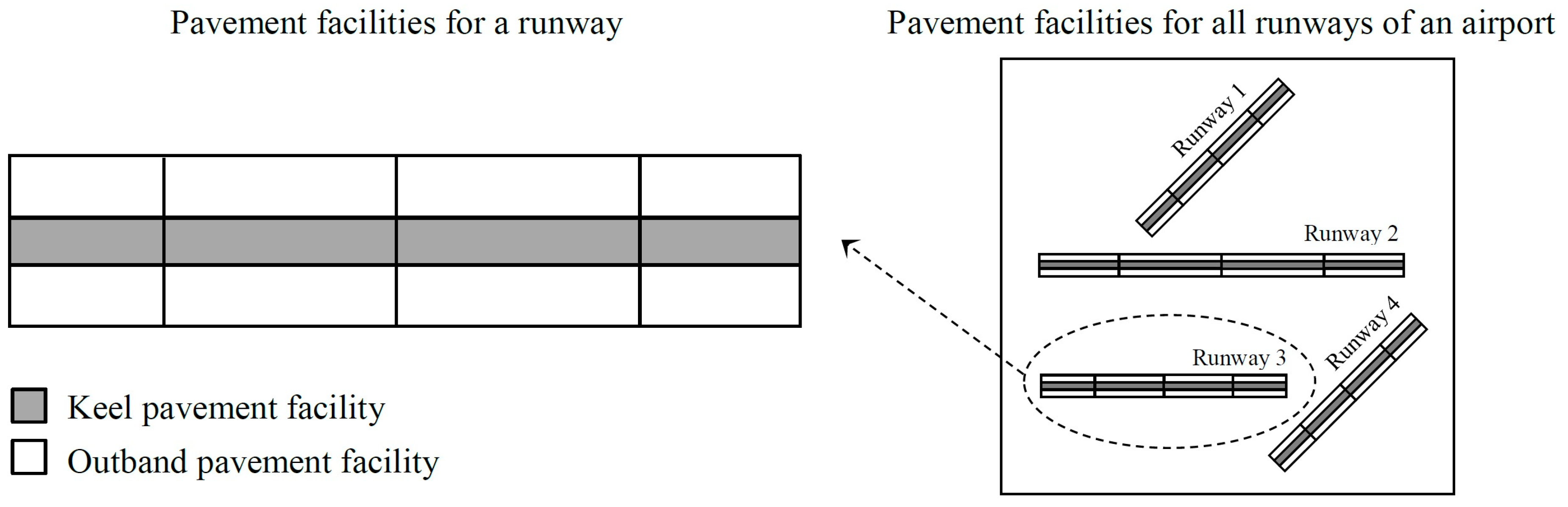
Maintaining airfield pavement conditions at satisfactory levels to ensure safe and efficient aircraft operations involves substantial funding for maintenance and rehabilitation (M&R). In the US national airport system, the amount of federal funding for runway rehabilitation alone accumulated to more than $5.1 billion between 2008 and 2017 [1]. How to spend the funding at major airports is generally directed by airport pavement management systems (APMSs), which rely on the PAVER software [2,3] to schedule M&R policies on pavement facilities (note: following the pavement management literature, the terms “M&R activities” and “M&R policies” are used interchangeably in the paper). In the airport pavement management literature, a pavement facility refers to the smallest pavement unit for condition assessment and M&R planning. Typically, a runway consists of multiple pavement facilities. As an illustration, in Figure 1 an airport has four runways. The pavement of Runway 3 is divided longitudinally and laterally into 12 facilities. The four facilities on the upper side and the four facilities on the lower side (in white) are termed outband pavement facilities. The four facilities in the middle (in grey) are termed keel pavement facilities. The lateral division is made to account for the channelization of aircraft traffic load across a runway [2].

While easy to understand, using PAVER to schedule M&R policies has limitations. First, PAVER recommends M&R policies on pavement facilities based on condition thresholds and prioritization rules. Specifically, for each pavement facility and in each year, PAVER assigns an M&R activity as a function of whether the condition of the facility is below a prescribed threshold. Then, the assigned M&R activities of all facilities are prioritized based on factors such as the urgency of an M&R type (e.g., patching should be performed whenever needed, to ensure safe aircraft operations) and pavement use (e.g., keel pavement facilities are given higher priority than outband facilities due to greater traffic loading) [3]. Obviously, such a threshold- and prioritization-based approach does not lead to an optimal use of the available budget. Moreover, in PAVER there is no mentioning that interdependence of M&R policies among pavement facilities is considered. For example, there may be an aggregate performance requirement that the percentage of facilities in a bad condition should not exceed some maximum permissible value [4]. Also, major M&R actions can impose runway closure for an extended period and thus disrupt aircraft operations. Thus, when considering a major M&R action, applying it to an entire runway would be better than to a single pavement facility or a portion of the runway so that disruptions to aircraft traffic can be minimized [4].

Second, scheduling M&R policies requires pavement condition forecast as inputs. PAVER uses simple extrapolation to yield deterministic pavement condition forecast, which is subject to criticism in three aspects: (1) simple extrapolation fails to take into full consideration the impact on pavement deterioration of pavement design characteristics (e.g., pavement surface type), past pavement conditions, and other exogenous factors such as historic M&R actions and traffic loads [5,6]; (2) predicting pavement deterioration deterministically is not realistic due to unobserved and uncapturable influencing factors and measurement error [7,8]; (3) the process of pavement deterioration is dynamic, meaning that pavement condition degradation may not be time-homogenous (i.e., stationary) but can speed up or slow down over time [9]. Consideration of the dynamics in pavement deterioration is missing in the state-of-the-practice.

To address the above limitations, two contributions are made in the paper. The first contribution is considerations of the interdependence of M&R policies among pavement facilities, reflected in: (1) aggregate pavement performance for each runway, meaning that the fraction of pavements of a runway in a bad condition must not exceed the maximum permissible value; (2) simultaneous implementation of a major M&R action on connected facilities, meaning that when a major M&R action is applied, it should be applied to an entire runway rather than a single pavement facility or a portion of the runway. In addition, in scheduling M&R policies the budget constraint is respected, i.e., the implementation of M&R policies among pavement facilities is constrained by the total available budget. The above interdependence considerations are incorporated in a network optimization-based M&R planning framework as described below.

The second contribution of the paper is made by proposing a new modeling approach, which integrates stochastic duration models to predict runway pavement conditions with a network optimization-based framework for scheduling M&R activities on the pavements. Stochastic duration models allow for capturing the stochastic and dynamic nature of pavement deterioration as influenced by pavement design, past performance, and other exogenous factors. The network optimization-based framework, which builds on pavement condition forecast produced by the stochastic duration models and the idea of simultaneous network optimization, provides an M&R plan for each pavement facility in the system while minimizing the overall M&R cost and considering the interdependence of M&R policies among facilities.

Development of the network optimization-based framework is motivated by the dimensionality challenge in M&R planning for a network of pavements. Given that there can be hundreds of runway pavement facilities at an airport and multiple M&R policies may be considered for each facility in each period over a planning horizon, the M&R decision space is extremely large. To tackle the dimensionality challenge, previous research approaches the system-level M&R planning problem from two levels. The first is at the financial planning level, which concerns optimal allocation of total budget to meet the system-level pavement performance standards [10,11]. The resulting M&R policy recommendations do not point to specific facilities, but only to the portions of facilities with the same condition. To translate such aggregate recommendations to facility-specific M&R policies, additional engineering judgement or subroutines will be needed but are often subjective. The second is at the operational planning level, aiming at scheduling facility-specific M&R decisions. M&R policies are determined for individual facilities first, and then adjusted to meet system-level constraints. The adjustment process, however, can compromise system-level optimality [12,13]. Thus, it is clear that a new approach to M&R planning is much needed to yield M&R policies that are both facility specific and system optimum while accounting for the interdependence of M&R policies among facilities in the context of airport runway pavement management. This paper seeks to find such an approach.

The advantage of the proposed modeling approach is demonstrated in a case study of Chicago O’Hare International airport. By estimating stochastic duration models, the probabilities for pavement condition transition between different states and time-dependent pavement deterioration curves are derived. By integrating the stochastic duration model estimates with the network optimization-based framework, significantly reduced M&R cost for O’Hare runway pavements is found compared to the current practice, at the same time achieving a high level of pavement performance.

The rest of the paper is organized as follows. The next section provides a review of the relevant research. This is ensued by the presentation of methodologies for pavement performance modeling and network optimization-based M&R planning framework. The results of applying the overall modeling approach to O’Hare airport are reported and discussed next. Finally, the paper concludes with a summary of key findings and suggestions for future work.

2. Background

The state-of-the-art methodologies to optimally schedule M&R activities for a network of pavement facilities are frequently based on Markov decision processes (MDPs) [10,14,15,16,17,18]. Broadly speaking, two approaches have been developed in the literature [2]: top-down and bottom-up approaches. The top-down approach takes into account the interdependence between M&R decisions across facilities so that network-level constraints such as budget limit and mandatory performance standards are satisfied [10,11,19]. Linear Programs (LP) are formulated under this approach to yield randomized M&R policies which give fractions of facilities that are in each condition state and recommended for an M&R activity. To make the solutions implementable, i.e., identification of facility-specific actions from the optimization results, additional subjective engineering judgement or subroutines will be needed to translate the randomized policies into facility-specific M&R policy recommendations.

Different from the top-down approach, the bottom-up approach aims to generate facility-specific M&R policies completely through optimization without the involvement of subjective engineering judgement or subroutines [20]. However, the optimization is subject to significant computational challenges (i.e., the curse of dimensionality) arising from the number of facilities to consider in an infrastructure network [21,22,23]. To overcome the challenges, decomposition techniques have been developed which first solve facility-level and then network-level problems. Because of the sequential nature, suboptimal decisions will result [12,13,24]. In the literature, heuristics such as genetic algorithms have also been used for problems with discrete condition states [25,26]. But again, solution optimality cannot be guaranteed using heuristics.

To bridge the gap between the top-down and the bottom-up MDP-based approaches in terms of operationality and optimality, recently Medury and Madanat [27] proposed the simultaneous network optimization (SNO) framework which jointly considers network-level constraints and facility-specific decisions through the formulation of mixed-integer linear programs (MILP). The salient feature of SNO is that it provides facility-specific M&R policies for the current year of decision-making while utilizing the randomized policies to compute the expected future costs. Using Monte Carlo simulations, facility-specific M&R policies for every year over the planning horizon can be obtained. In addition, the MILP under SNO can be solved very fast, thus evading the curse of dimensionality faced by the bottom-up approach. Nazari et al. [28] further incorporated infrastructure inspection scheduling and measurement error into SNO.

Given the ability of SNO to deal with both operationality and optimality in M&R planning for a network of pavement facilities, this paper follows the general idea of SNO. In generating facility-specific M&R policies, the proposed modeling approach extends the SNO framework by accounting for the interdependence of M&R policies among pavement facilities as required for airport runway pavement management. The SNO framework is further adapted to incorporate a non-stationary MDP which characterizes the stochasticity and dynamics of pavement deterioration, and the spatial and type heterogeneity of pavement facilities.

In modeling infrastructure deterioration, various approaches have been adopted in previous studies using historic condition assessment data. The approaches include the estimation/use of nonlinear regression models [29], the expected value method [14,30,31], Poisson regression [8], Probit models [32,33], mixed-logit models [34], joint discrete-continuous models [7], stochastic duration models [5,35,36,37], Bayesian approach [38,39,40], and neuro-fuzzy models [41,42]. Besides, the effectiveness of M&R activities on infrastructure performance has been considered using single-equation models of infrastructure performance and maintenance [43], sequential equation models [44], simultaneous equation models [45,46], and time-series models [47,48,49].

3. Methodology

In this section, stochastic duration models to predict pavement performance are first presented. Building on the stochastic duration models, an M&R planning framework is put forward that optimally schedules M&R activities, in the context of an airport runway pavement network. A runway pavement network consists of multiple runways $j\in J$. Note that the presented M&R planning framework is general enough and can be applied to a whole airfield pavement network comprising runways, taxiways, aprons, and roadways. Doing so would only require defining each $j\in J$ as a runway, a taxiway, an apron, or a roadway, with no further change in the modeling framework. While in this paper only runways are considered (as suggested by O’Hare airport engineers when the research was conducted), it does not limit the possibility to apply the framework to a broader range of airport pavement assets. Recalling Figure 1, each runway is divided into multiple pavement facilities $i\in I$, such that each facility exhibits identical characteristics in terms of pavement surface/material type $m\in M$, construction time, etc. The lateral location of a pavement facility, which can be either outband or keel, is denoted by $l\in L=\left\{\mathrm{keel},\mathrm{outband}\right\}$.

The stochastic duration models and the M&R planning framework are based on finite-horizon discrete-state MDPs. At the beginning of each year $\tau$ over a planning horizon that ends at year $T$, the performance of each pavement facility is characterized by a condition state $s\in S$ and an M&R action $a\in A$ is scheduled for the facility. To facilitate exposition, the following notations are introduced (

Table 1. Notations.

Sets
$A$	M&R actions including the “do-nothing” alternative $\left(a\in A\right)$
$S$	condition states $\left(s\in S\right)$
$J$	runways $\left(j\in J\right)$
$I$	pavement facilities $\left(i\in I\right)$
$L$	cross-sectional locations of facilities ($l\in L=$ {keel, outband})
$M$	$\mathrm{pavement}\mathrm{surfaces}/\mathrm{material}\mathrm{types}\left(m\in M\right)$
$N$	pavement age in a condition state (age-in-state) $\left(n\in N\right)$
Variables
$x_{i,a,\tau }$	1 if action $a$ is selected for facility $i$ during year $\tau$; 0 otherwise
$w_{s,a,\tau }^{j,l,m,n}$	fraction of facilities on runway $j$ that are located on cross-section $l$, paved with material $m$, and in condition state $s$ for $n$ years, to which action $a$ is applied during year $\tau$
Parameters
${𝕤}_{\tau }\left(i\right)$	condition state of facility $i$ at the beginning of year $\tau$
${𝕞}_{\tau }\left(i\right)$	material type of facility $i$ at the beginning of year $\tau$
${𝕟}_{\tau }\left(i\right)$	age-in-state of facility $i$ at the beginning of year $\tau$
$B_{\tau }$	annual budget in year $\tau$
$c\left(s,a\right)$	unit cost of implementing action $a$ when a facility is in state $s$
${\rho }_i$	area of facility $i$
${\gamma }_j$	area of runway $j$
$f_s^{\max }$	maximum acceptable fraction of facilities on each runway in condition state $s$
${\pi }_a^{l,m,n}\left(s^{\prime },s\right)$	transition probability from state $s^{\prime }$ to $s$ of facilities located on cross-section $l$, paved with material $m$, and with age-in-state $n$ if action $a$ is applied
${\varphi }_a\left(m^{\prime },m\right)$	binary indicator of material change, equal to 1 if action $a$ replaces material $m^{\prime }$ with material $m$; 0 otherwise
${\phi }_a\left(n^{\prime },n|s^{\prime },s\right)$	binary indicator of age-in-state change, equal to 1 in either of two situations: (1) a state transition from $s^{\prime }$ to $s$ ($s^{\prime }\ne s$) with action a and age-in-state changes from $n^{\prime }$ to $n=0$; (2) no state transition ($s^{\prime }=s$): age-in-state changes from $n^{\prime }$ to either $n=n^{\prime }+1$ with a minor action $a$ or $n=0$ with a major action $a$; 0 otherwise
${\delta }_{i,j}$	1 if facility $i$ is located on runway $j$; 0 otherwise
${\zeta }_{i,l}$	1 if facility $i$ is located on cross-section $l$; 0 otherwise
${\eta }_{a,m}$	1 if action $a$ is not compatible with material $m$; 0 otherwise

).

3.1. Pavement Condition Forecast with Stochastic Duration Models

In discrete-state discrete-time MDPs, the evolution of pavement performance with transition probabilities needs to be characterized. More specifically, knowing the condition state of a facility at the beginning of time period $\tau$ and an M&R action taken during the time period, the likely condition states and their probabilities at the start of the next time period $\tau +\Delta$ is given by the corresponding transition probabilities. $\Delta$ is the time interval between consecutive inspections of pavement conditions (e.g., $\Delta =1$ year). To construct the transition probabilities, continuous-time stochastic duration models are estimated.

The dependent variable in stochastic duration models is the state duration, which refers to the time it takes a pavement facility to leave a specific condition state after entering that state. Let $D_s$ denote a non-negative continuous random variable representing the duration of a facility in state $s\in S$. As shown in Equation (1), the probability of leaving state $s$ at any point in time $d$ is the probability of observing a worse state at time $d+\Delta$, conditional on the observed state of $s$ at time $d$. The conditional probability in Equation (1) recognizes that the likelihood of a facility to leave a state can depend on the length of the elapsed time since the facility entered the state. Therefore, the assumption of independence from history, often referred to as the memoryless (Markovian) property, is relaxed in stochastic duration models.

$$P_s\left(d,\Delta \right)=Pr\left(d\le D_s<d+\Delta |D_s>d\right)=\frac{Pr\left(d\le D_s<d+\Delta \right)}{Pr\left(D_s>d\right)}=\frac{F_s\left(d+\Delta \right)-F_s\left(d\right)}{{\overline{F}}_s\left(d\right)}$$

(1)

where ${\overline{F}}_s\left(d\right)$ is the survival function of state $s$, which is the probability that the duration of staying in state $s$ is at least $d$: ${\overline{F}}_s\left(d\right)=Pr\left(D_s>d\right)=1-F_s\left(d\right)$, where $F_s\left(d\right)$ is the cumulative distribution function of $D_s$.

Given that the probability of leaving state $s$ at time $d$, $P_s\left(d,\Delta \right)$, depends on the interval $\Delta$, an average rate of transition out of state $s$ can be obtained by dividing $P_s\left(d,\Delta \right)$ by $\Delta$. For very small values of $\Delta$, Equation (2) defines the hazard rate at time $d$, $h_s\left(d\right)$, which refers to the instantaneous rate of leaving state $s$. The shape of the hazard rate function (i.e., how the duration of a state depends on the length of the elapsed time since entering that state) has important implications for the dynamics of duration. A monotonically increasing/decreasing hazard rate function indicates that the conditional probability of transition out of state $s$ increases/decreases with the time already spent in that state. A constant hazard rate function implies a duration-independent stochastic process, which suggests that the Markovian memoryless property holds [50]. Therefore, the validity of the Markovian assumption can be tested using stochastic duration models.

$$h_s\left(d\right)=\underset{\Delta \to 0^{+}}{\lim }\frac{P_s\left(d,\Delta \right)}{\Delta }=\underset{\Delta \to 0^{+}}{\lim }\frac{F_s\left(d+\Delta \right)-F_s\left(d\right)}{\Delta {\overline{F}}_s\left(d\right)}=\frac{f_s\left(d\right)}{{\overline{F}}_s\left(d\right)}$$

(2)

where $f_s\left(d\right)$ is the probability density function (PDF) of the random variable $D_s$.

It is obvious from Equation (2) that the hazard rate can be computed once the distribution of the random variable $D_s$ is known. To account for the possible types of duration dependence (i.e., increasing/decreasing/constant), it is assumed that the state duration follows Weibull distribution $D_s~W\left(\lambda ,p\right)$, where $\lambda >0$ and $p>0$ are respectively the location and scale parameters of Weibull distribution that should be estimated. $p>1$ implies an increasing hazard rate with the time in state, $p<1$ indicates a decreasing hazard rate with the time in state, and $p=1$ suggests a constant hazard rate over time. The hazard rate function corresponding to Weibull distribution is obtained in Equation (3).

$$h_s\left(d\right)=\lambda p{\left(\lambda d\right)}^{p-1}$$

(3)

Recall from the Introduction section that pavement condition may depend on pavement design characteristics and exogenous factors (such as maintenance history and traffic load) in addition to the time already spent in a condition state. The external factors are incorporated into the hazard rate function by replacing the constant Weibull parameter $\lambda >0$ with a strictly positive function of exogenous variables such as $\lambda =e^{-p\mathit{\beta }\mathit{Y}}$. $\mathit{Y}=\left[Y_1,Y_2,\dots ,Y_k\right]$ is the vector of explanatory variables ($k$ is the index of exogenous variables) and $\mathit{\beta }={\left[{\beta }_1,{\beta }_2,\dots ,{\beta }_k\right]}^T$ is the vector of the corresponding coefficients that should be estimated. Plugging this exponential function into Equation (3) yields:

$$h_s\left(d\right)=p.e^{-p\mathit{\beta }\mathit{Y}}.d^{p-1}$$

(4)

The parameters $p$ and $\mathit{\beta }$ in Equation (4) are estimated from a time series of condition state observations and the associated state durations $D_s$, $\forall s\in S$, of pavement facilities. However, the state duration may be unknown for some facilities if the state transition has not yet happened by the latest observation time. These observations are called censored data and the phenomenon is referred to right censoring, where it is only known that the state duration is greater than a number [50]. Therefore, it is crucial to incorporate and treat censored data in estimating duration model parameters. To this end, the maximum likelihood estimation method [35,50] is used, as shown in Equation (5), which gives estimates for $p$ and $\mathit{\beta }$ that maximize the log-likelihood function $L{L}_s\left(p,\mathit{\beta }\right)$. In this method, all possible parameter values for a specified model are searched to find the set of values such that the observed sample is most likely in the probabilistic sense. That is, the set of parameter values that, given a model, is most likely to give us the data.

$$L{L}_s\left(p,\mathit{\beta }\right)={\displaystyle \sum }_{\mathrm{uncensored}}\ln f_s\left(d|\mathit{Y},p,\mathit{\beta }\right)+{\displaystyle \sum }_{\mathrm{right}\mathrm{censored}}\ln {\overline{F}}_s\left(d|\mathit{Y},p,\mathit{\beta }\right)$$

(5)

Using the estimation results of continuous-time duration models, the transition probabilities of discrete-time MDPs can then be computed. Consider a pavement facility in condition state $s\in S$ at time $d$ and an inspection interval $\Delta$. The objective is to find the probabilities of either remaining in or leaving $s$ with a mild assumption that at most two drops in state can occur in the period $\Delta$ [5]. The probability of remaining in state $s$ over the period $\Delta$, $\pi \left(s,s\right)$, is simply $1-P_s\left(d,\Delta \right)$, where $P_s\left(d,\Delta \right)$ is the conditional probability of leaving state $s$ (see Equation (1)). For presentation purposes, the subscripts and superscripts of ${\pi }_a^{l,m,n}\left(s^{\prime },s\right)$ are omitted in this section.

$$\pi \left(s,s\right)=1-P_s\left(d,\Delta \right)=\frac{{\overline{F}}_s\left(d+\Delta \right)}{{\overline{F}}_s\left(d\right)}$$

(6)

Equation (6) can be further simplified by defining the integrated hazard rate function ${\mathsf{\Lambda }}_s\left(d\right)={{\displaystyle \int }}_0^d{h}_s\left(x\right)\mathrm{d}x$, and re-writing Equation (2) as $h_s\left(d\right)=\frac{-\mathrm{d}\ln {\overline{F}}_s\left(d\right)}{\mathrm{d}d}$. Consequently, ${\overline{F}}_s\left(d\right)=\exp \left(-{\mathsf{\Lambda }}_s\left(d\right)\right)$. Specific to a Weibull distribution, ${\mathsf{\Lambda }}_s\left(d\right)$ would be equal to ${\left(\lambda d\right)}^p$ and consequently ${\overline{F}}_s\left(d\right)=\exp \left(-{\lambda }^p{d}^p\right)$. $\pi \left(s,s\right)=\exp \{{\lambda }^p\left[d^p-{\left(d+\Delta \right)}^p\right]$}.

The probability of one drop in state $s$ to the next worse state $s+1$ over the period $\Delta$, $\pi \left(s,s+1\right)$, equals the probability of observing state $s+1$ at time $d+\Delta$ given that state $s$ was observed at time $d$. To this end, the duration in state $s+1$ has to be larger than the interval between the state transition time and the end of the period $\Delta$. If state transition happens at some time $u$ between $d$ and $d+\Delta$, the transition probability $\pi \left(s,s+1\right)$ will be the product of two probabilities: the probability of the transition out of state $s$ taking place at $u$, and the probability that the duration of state $s+1$ is greater than $d+\Delta -u$. An integral is then taken over the state transition time $u$ between $d$ and $d+\Delta$ to obtain the transition probability $\pi \left(s,s+1\right)$, as follows:

$$\pi \left(s,s+1\right)={{\displaystyle \int }}_d^{d+\Delta }Pr\left(u\le D_s\le u+\mathrm{d}u|D_s>d\right)Pr\left(D_{s+1}>d+\Delta -u\right)\mathrm{d}u$$

$$={{\displaystyle \int }}_d^{d+\Delta }\frac{F_s\left(u+\mathrm{d}u\right)-F_s\left(u\right)}{{\overline{F}}_s\left(d\right)}{\overline{F}}_{s+1}\left(d+\Delta -u\right)\mathrm{d}u$$

(7)

Finally, the probability of transitioning to the next two worse state $s+2$ over the period $\Delta$ is obtained as follows.

$$\pi \left(s,s+2\right)=1-\pi \left(s,s\right)-\pi \left(s,s+1\right)$$

(8)

3.2. Network Optimization-Based Framework for M&R Planning

3.2.1. Basic Idea

This section presents a planning framework to schedule M&R actions on each facility for a network of airfield runway pavements, such that the total M&R cost, which is the sum of present and expected future M&R costs over a planning horizon, is minimized. The SNO framework is adopted with extensions to: (1) account for the interdependence of M&R policies among pavement facilities, and (2) incorporate a non-stationary MDP to characterize the stochasticity and dynamics of pavement deterioration and the spatial and type heterogeneity of pavement facilities. The idea of minimizing total M&R cost over a planning horizon is in line with the infrastructure management literature [6,21,51,52,53].

It is worth noting that the basic idea behind the framework is not different from an alternative view of M&R action planning which is to minimize the gap between the design life-cycle cost and the actual life-cycle cost. More specifically, standing at the current time, the life-cycle cost consists of: (1) construction and M&R costs incurred from the start of the life cycle up to the current time; and (2) current and expected future M&R costs up to the end of the life cycle. Let $A$ and $C$ denote respectively the design life cycle costs for the period from the start of the life cycle up to the current time and for the period from the current time to the end of the life cycle. Similarly, $B$ and $D$ are used to represent the actual life cycle costs for the two periods. Because $A$ and $C$ would be determined prior to the life cycle, it is reasonable to assume that $A+C$ is the ideal, i.e., the minimum possible, life-cycle cost. Minimizing the gap between the actual and the design life-cycle costs is expressed as $\min \left(B+D\right)-\left(A+C\right)$.

At the current time when decisions on current and future M&R activities are to be made, $A$ and $C$ are known (as they would be determined prior to the life cycle). $B$ is obviously also known as it is the cost incurred in the past. Thus $A$, $B$, and $C$ are constant at the current time. The above minimization then reduces to $\min D$, which is minimizing the current and expected future M&R costs, as concerned in the proposed framework.

3.2.2. Model Formulation

We consider solving mixed-integer linear program (MILP) (9)–(18) to obtain the optimal M&R action for each facility in year $t$. For future years from $t+1$ till the end of the planning horizon $T$, the MILP provides randomized policies. As described in detail in the next subsection, in scheduling M&R actions, the MILP needs to be solved for each year from the current year $t$ till the end of the planning horizon $T$.

The decision variables of the MILP are $x_{i,a,t}$ and $w_{s,a,\tau }^{j,l,m,n}$. For year $t$, binary decision variables $x_{i,a,t}$ indicate whether M&R action $a\in A$ is recommended for facility $i\in I$. For years $\tau =t,\dots ,T+1$, randomized policies $w_{s,a,\tau }^{j,l,m,n}$ refer to the fraction of facilities on runway $j$ that are located on cross-sectional location $l$, paved with material $m$, and in condition state $s$ for $n$ years, to which action $a$ is applied during year $\tau$.

Note that because the start of the planning horizon (i.e., $\tau =t$) does not necessarily coincide with the origin of time-in-state $s$, a separate index $n\in N$ is defined to represent the age-in-state, where $N$ is the set of possible age-in-state values. The integer-valued age-in-state $n$ is related to the real-valued time-in-state $D_s\ge 0$ in the previous subsection by $n=⎣D_s⎦$, where ⎣$.$⎦ is the floor function giving the integer part of a real number. For example, if the observed time-in-state of a facility is 3 years and 4 months, an age-in-state of 3 years is assumed. The definition of randomized policies on indices $l$, $m$, and $n$ aims to capture respectively the spatial heterogeneity (i.e., keel vs. outband locations), surface/material type heterogeneity, and time heterogeneity (i.e., non-stationary deterioration process).

$$\underset{x,w}{\min }{\displaystyle \sum }_{i\in I}{\displaystyle \sum }_{a\in A}c\left({𝕤}_t\left(i\right),a\right){\rho }_i{x}_{i,a,t}+{\displaystyle \sum }_{j\in J}{\displaystyle \sum }_{l\in L}{\displaystyle \sum }_{m\in M}{\displaystyle \sum }_{n\in N}{\displaystyle \sum }_{s\in S}{\displaystyle \sum }_{a\in A}{\displaystyle \sum }_{\tau =t+1}^{T}c\left(s,a\right){\gamma }_j{w}_{s,a,\tau }^{j,l,m,n}$$

(9)

s.t.

$$x_{i,a,t}\in \left\{0,1\right\}\hspace{1em}\hspace{1em}\forall i\in I;a\in A$$

(10)

$$w_{s,a,\tau }^{j,l,m,n}\ge 0\hspace{1em}\hspace{1em}\forall j\in J;l\in L;m\in M;n\in N;s\in S;a\in A;\tau =t+1,\dots ,T$$

(11)

$${\displaystyle \sum }_{l\in L}{\displaystyle \sum }_{m\in M}{\displaystyle \sum }_{n\in N}{\displaystyle \sum }_{s\in S}{\displaystyle \sum }_{a\in A}{w}_{s,a,\tau }^{j,l,m,n}=1\hspace{1em}\hspace{1em}\forall j\in J;\tau =t+1,\dots ,T$$

(12)

$${\displaystyle \sum }_{a\in A}{x}_{i,a,t}=1\hspace{1em}\hspace{1em}\forall i\in I$$

(13)

$$w_{s,a,t}^{j,l,m,n}=\frac{1}{{\gamma }_j}{\displaystyle \sum }_{i\in I|{𝕤}_t\left(i\right)=s,{𝕞}_t\left(i\right)=m,{𝕟}_t\left(i\right)=n}{\delta }_{i,j}{\zeta }_{i,l}{\rho }_i{x}_{i,a,t}\hspace{1em}\hspace{1em}\forall j\in J;l\in L;m\in M;n\in N;s\in S;a\in A$$

(14)

$${\displaystyle \sum }_{m^{\prime }\in M}{\displaystyle \sum }_{n^{\prime }\in N}{\displaystyle \sum }_{s^{\prime }\in S}{\displaystyle \sum }_{a\in A}{\varphi }_a\left(m^{\prime },m\right){\phi }_a\left(n^{\prime },n|s^{\prime },s\right){\pi }_a^{l,m^{\prime },n^{\prime }}\left(s^{\prime },s\right)w_{s^{\prime },a,\tau }^{j,l,m^{\prime },n^{\prime }}={\displaystyle \sum }_{a\in A}{w}_{s,a,\tau +1}^{j,l,m,n}$$

(15)

$$\forall j\in J;l\in L;m\in M;n\in N;s\in S;\tau =t,\dots ,T$$

$${\displaystyle \sum }_{j\in J}{\displaystyle \sum }_{l\in L}{\displaystyle \sum }_{m\in M}{\displaystyle \sum }_{n\in N}{\displaystyle \sum }_{s\in S}{\displaystyle \sum }_{a\in A}c\left(s,a\right){\gamma }_j{w}_{s,a,\tau }^{j,l,m,n}\le B_{\tau }\hspace{1em}\hspace{1em}\forall \tau =t,\dots ,T$$

(16)

$${\displaystyle \sum }_{l\in L}{\displaystyle \sum }_{m\in M}{\displaystyle \sum }_{n\in N}{\displaystyle \sum }_{a\in A}{w}_{s,a,\tau }^{j,l,m,n}\le f_s^{\max }\hspace{1em}\hspace{1em}\forall j\in J;s\in S;\tau =t+1,\dots ,T+1$$

(17)

$${\displaystyle \sum }_{j\in J}{\displaystyle \sum }_{l\in L}{\displaystyle \sum }_{m\in M}{\displaystyle \sum }_{n\in N}{\displaystyle \sum }_{s\in S}{\displaystyle \sum }_{a\in A}{\displaystyle \sum }_{\tau =t}^T{\eta }_{a,m}{w}_{s,a,\tau }^{j,l,m,n}=0$$

(18)

where the area of a runway $j$ is computed as ${\gamma }_j={\displaystyle \sum }_{i\in I}{\delta }_{i,j}{\rho }_i$ given the area of pavement facility $i$, ${\rho }_i$, and facility-runway correspondence indicator ${\delta }_{i,j}$.

The objective function (9) minimizes the sum of M&R cost in year $t$ and expected future cost from $t+1$ till $T$, the end of the planning horizon. The first term is the cost of facility-specific M&R actions in year $t$. The second term represents the sum of expected future M&R costs using randomized policies $w_{s,a,\tau }^{j,l,m,n}$. Constraint (10) stipulates that $x_{i,a,t}$’s are binary. Constraints (11)–(12) ensure that the non-negative randomized policies associated with each runway will sum up to one each year. Constraint (13) guarantees that only one M&R action (including do-nothing) will be selected for each facility in year $t$. The relationship between the binary facility-specific variables $x_{i,a,t}$ and the randomized policies $w_{s,a,t}^{j,l,m,n}$ in year $t$ is established in constraint (14). Note that the relationship is runway specific. The summation on the right-hand side of constraint (14) is performed over those facilities that are in condition state $s$, paved with material $m$, and with age-in-state $n$ at the beginning of year $t$.

Constraint (15) builds on the Chapman-Kolmogorov relationship by relating the randomized policies of a given year with the policies of the subsequent year. It is also more complicated than the conventional Chapman-Kolmogorov relationship in that it reflects the characteristics of airport pavement M&R in greater detail—capturing not only the evolution of condition state but also the evolutions of material type and age-in-state over time. This is realized by using the transition probabilities derived in the previous sub-section, and the indicators of change in material type ${\varphi }_a\left(m^{\prime },m\right)$ and evolution of age-in-state ${\phi }_a\left(n^{\prime },n|s^{\prime },s\right)$. ${\varphi }_a\left(m^{\prime },m\right)$ is a binary indicator of pavement material change, taking value 1 if action $a$ replaces material $m^{\prime }$ with $m$, and 0 otherwise. ${\phi }_a\left(n^{\prime },n|s^{\prime },s\right)$ is a binary indicator of age-in-state evolution, which equals 1 if the age-in-state of a pavement facility changes from $n^{\prime }$ to $n$ during two consecutive years, given the state transition from $s^{\prime }$ to $s$ (including $s^{\prime }=s$) and the implementation of action $a$. Two cases can make ${\phi }_a\left(n^{\prime },n|s^{\prime },s\right)$ equal to 1: (1) condition state does not change with action $a$: $s=s^{\prime }$ and $n=n^{\prime }+1$; (2) condition state changes from $s^{\prime }$ to $s$ with action $a$ and $n=0$.

The maximum budget in each year and the permissible fraction of facilities on a runway in each condition state are enforced by constraints (16)–(17). The two constraints reflect the interdependence of M&R policies among the pavement facilities. Constraint (17) may come from airlines to ensure aircraft operational safety which relates to pavement conditions. Note that constraint (17) enforces performance standards on each runway individually. This is possible as the randomized policies $w_{s,a,\tau }^{j,l,m,n}$ are defined in such a way that $w_{s,a,\tau }^{j,l,m,n}$’s sum up to one for each runway $j\in J$ (see constraint (12)). Finally, because each material type is compatible with only some M&R actions, constraint (18) is used to prescribe all the M&R actions that are incompatible with a pavement material. ${\eta }_{a,m}$ is a binary indicator that is equal to 1 if action $a$ is not compatible with material $m$ and is 0 otherwise.

Another reflection of the interdependence of M&R policies among pavement facilities is about simultaneous implementation of a major M&R action on connected facilities. While minor M&R activities are conducted mostly during periods when aircraft traffic is low (e.g., at night) and disruption to aircraft operations is minimal, major M&R actions (e.g., rehabilitation) could interrupt airport operations as they may not be implemented over night. To minimize disruptions, an airport authority may apply a major M&R action to an entire runway if decided, rather than to only one pavement facility within the runway [4]. This is enforced by adding constraint (19) into the MILP.

$$x_{i,a,t}\ge {\displaystyle \sum }_{j\in J}{\displaystyle \sum }_{l\in L}{\displaystyle \sum }_{n\in N}{\displaystyle \sum }_{s\in S}{\delta }_{i,j}{w}_{s,a,t}^{j,l,{𝕞}_t\left(i\right),n}\hspace{1em}\hspace{1em}\forall i\in I;a\in A^{\mathrm{major}}$$

(19)

In constrain (19), the summation on the right-hand side is only on the randomized policies associated with the same material type as for facility $i$ in year $t$, given that each runway may be composed of facilities with heterogeneous materials.

It should be noted that constraint (19) only applies to the current year $t$ when solving the MILP (for future years, randomized policies $w_{s,a,\tau }^{j,l,m,n}$ ($\tau =t+1,\dots ,T$) are used). This is a limitation of the SNO framework if the simultaneous implementation of a major M&R action on connected facilities must be accounted for throughout the planning horizon. The authors’ future work intends to devise ways to overcome this limitation, for example, by incorporating approximate dynamic programming into the M&R planning framework [54].

3.2.3. Obtaining Facility-Specific M&R Recommendations over a Planning Horizon

The MILP (9)–(18)/(19) introduced in the previous subsection will be applied to obtain facility-specific M&R policies every year over a planning horizon. More specifically, at the beginning of each year in the planning horizon, the M&R policy to be implemented on each pavement facility in that year will be determined by solving a corresponding MILP (9)–(18)/(19). Doing so will utilize knowledge about the realized material type, condition state, and age-in-state of each pavement facility at the beginning of that year, i.e., ${𝕞}_{\tau }\left(i\right)$, ${𝕤}_{\tau }\left(i\right)$, and ${𝕟}_{\tau }\left(i\right)$, $\forall \tau =t,t+1,\dots ,T$. At the beginning of the planning horizon, however, the condition state transition of each facility is stochastic, suggesting that only ${𝕞}_t\left(i\right)$, ${𝕤}_t\left(i\right)$, and ${𝕟}_t\left(i\right)$ are known with certainty. Thus Monte Carlo simulation [55] is employed, as detailed below.

Given the material type of each facility ${𝕞}_{\tau }\left(i\right)$ and the corresponding optimal policy $a_{\tau }$ for a year $\tau$, the material type of the facility at the beginning of year $\tau +1$, ${𝕞}_{\tau +1}\left(i\right)$, can be determined using the binary indicator ${\varphi }_a\left(m^{\prime },m\right)=1$, where $m^{\prime }={𝕞}_{\tau }\left(i\right)$ and $m={𝕞}_{\tau +1}\left(i\right)$. Given further the realized condition state of each facility ${𝕤}_{\tau }\left(i\right)$ for year $\tau$, the condition state of the facility at the beginning of year $\tau +1$, ${𝕤}_{\tau +1}\left(i\right)$, is generated using a uniform (0,1) random number generator and the transition probability distribution ${\pi }_a^{l,m^{\prime },n^{\prime }}\left({𝕤}_{\tau }\left(i\right),{𝕤}_{\tau +1}\left(i\right)\right)$, where $n^{\prime }={𝕟}_{\tau }\left(i\right)$. Then the age-in-state of the facility at the beginning of year $\tau +1$, ${𝕟}_{\tau +1}\left(i\right)$, is obtained based on the age-in-state of the previous year ${𝕟}_{\tau }\left(i\right)$, the condition state of the previous year ${𝕤}_{\tau }\left(i\right)$, and the simulated condition state of the given year ${𝕤}_{\tau +1}\left(i\right)$.

With ${𝕞}_{\tau +1}\left(i\right)$, ${𝕤}_{\tau +1}\left(i\right)$, and ${𝕟}_{\tau +1}\left(i\right)$, the optimal policies $a_{\tau +1}$ for all facilities are solved for using MILP (9)–(18). Iterating this procedure until the end of the planning horizon, the final outcome is a sample realization of condition state-action pairs over time, i.e., $\left\{\left({𝕤}_t,a_t\right),\left({𝕤}_{t+1},a_{t+1}\right),\dots ,\left({𝕤}_T,a_T\right),{𝕤}_{T+1}\right\}$. The process is repeated for a number of times such that the averaged sum of simulated costs in each of the future years $t+1,t+2,\dots ,T+1$ becomes close to the total expected future cost by solving the MILP (9)–(18) for the first year $t$. The same iterative procedure for each simulation and the same number of simulation runs are performed when constraint (19) is further considered.

4. Application at Chicago O’Hare Airport

In this section, the modeling approach is applied to runway pavement management at Chicago O’Hare International airport. The runway pavement database at O’Hare includes condition measurements, M&R history, and other pavement characteristics (e.g., construction/rehabilitation date and surface/material). As shown in

Table 2. Summary statistics of runway pavement assets at O’Hare International airport (2015).

Runway Code	Area (000 sq. meters)	No. of Facilities	Surface (% area)		Condition (% area)
			PCC *	APC **	State 1	State 2	State 3
R9R	113.7	28	21.76	78.24	41.31	58.69	0
R9L	104.5	9	100	0	100	0	0
R4R	112.5	9	0	100	100	0	0
R4L	99.2	34	0	100	87.97	11.55	0.48
R14R	180.9	24	0	100	90.46	9.54	0
R10L	182.1	21	29.67	70.33	59.66	40.34	0
R10C	186.8	19	100	0	100	0	0
sum	979.7	144	37.77	62.23	82.71	17.24	0.05

* PCC: Portland Cement Concrete. ** APC: Asphalt Concrete on PCC.

, in 2015 the airport has seven active runways, which are divided into 144 pavement facilities that cover more than 10.5 million square feet (i.e., 242 acres) of the airfield. Though all runways at the airport were (re)constructed with Portland Cement Concrete (PCC), Table 2 shows that almost 62% of the runway area have been resurfaced with asphalt concrete over time (we denote these facilities with Asphalt overlay on PCC, or APC). Pavement conditions have been routinely inspected and documented using the Pavement Condition Index (PCI), which combines data on individual distress types into a single condition value that ranges from 0 (worst) to 100 (best). The PCI value of a pavement facility is determined based on visual surveys of the number and type of distresses in the facility. Thus PCI already encompasses all distress effects. On the other hand, recommending M&R activities based on the types and sources of distress would not be possible for future years, as the types and sources of pavement distress cannot be adequately predicted, especially given that the planning horizon considered in the paper goes far into the future.

In this paper, a new discrete condition state variable is defined based on the documented PCI values and the thresholds set by O’Hare airport engineers. Specifically, for PCI values above 75, the condition state variable takes value one and the pavement is considered in the best state. If PCI is between 51 and 75, the condition state variable is given value two. If PCI is below 51, then the condition state variable is given value three. In Table 2, it can be seen that almost 83% of the runway area is currently in the best condition state, while less than 1% belongs to the worst state.

Based on the available information on the historic M&R actions and the comments made by the airport engineers, two (major) rehabilitation actions (1. PCC slab replacement; and 2. asphalt overlay) and three (minor) maintenance actions (1. PCC patching; 2. APC patching; and 3. APC crack sealing) are considered. Two points are worth noting. First, if one of the two rehabilitation actions (PCC slab replacement and asphalt overlay) is implemented, a pavement facility will be treated as new in state 1. This is supported by the historic evidence of the effectiveness of these two actions and the judgement by the airport engineers. Second, asphalt overlay is compatible with both PCC and APC pavements, whereas PCC slab replacement can be applied to PCC pavements only. Reconstruction is excluded from the set of feasible policies following the suggestion of the airport engineers due to the potentially significant impact on flight operations with a runway removed from service for a considerable period for reconstruction.

The unit cost associated with each M&R action, taken directly from O’Hare airport, is reported in

Table 3. M&R actions and the associated unit costs.

M&R Policy	Surface Compatibility	Unit Cost
Do-nothing	PCC, APC	$0	/sq. meter
Asphalt overlay	PCC, APC	$64.13	/sq. meter
APC patching	APC	$339.48	/sq. meter
APC crack sealing	APC	$14.76	/meter *
PCC slab replacement	PCC	$433.95	/sq. meter
PCC patching	PCC	$717.26	/sq. meter

* The linear unit cost of APC crack sealing is converted to an equivalent area unit cost based on the historic records.

. Note that the numbers for minor M&R actions in Table 3 refer to the unit cost of an action if implemented on a whole area unit (except for APC crack sealing, for which the unit cost is per unit length). On the other hand, in reality a minor M&R action would be implemented only on a small portion of the whole area of a runway pavement facility. Taking this into consideration, the M&R cost of a minor action on a pavement facility is calculated by multiplying the unit cost by the average portion of the pavement facility area that is subject to the minor action, which comes from the historic M&R records. So, while the unit cost number appears greater for a minor M&R action than for a major action (e.g., APC patching vs. Asphalt overlay), the calculated M&R cost of a pavement facility will be lower for a minor action than for a major action.

It is worth mentioning that maintenance management practice such as preference of night over day time to minimize traffic disruption and anti-icing/de-icing during winter times at the airport could play a vital role in affecting pavement management decisions in the agency cost dimension. On the other hand, the time dimension considered in the paper is by year (i.e., the model determines what M&R activities should be performed on which year), but not specific time points within a year. As the cost number for performing a specific M&R action within a year is directly taken from O’Hare airport, the number should already reflect the cost associated with the airport’s specific maintenance management practices.

4.1. Estimation Results of the Stochastic Duration Models

Separate models are estimated for the duration in each condition state to reflect the likely different mechanistic deterioration processes and different effects of causal factors on the duration in each state. Since three condition states are considered and each stochastic duration model gives the probability of transition out of a specific state to the other states, only models for transitions departing from states 1 and 2 need to be estimated (if a pavement is already in condition state 3, it cannot be worse). The effectiveness of the minor M&R actions is investigated by incorporating them into the duration models as causal factors. The stochastic duration models are estimated using the maximum likelihood estimation procedure described in the Methodology section, which is performed in the statistical software Stata.

Recall from the Methodology section that the dependent variable of stochastic duration models is the state duration. Therefore, a time variable is defined for each observation (which refers to the inspection outcome for a pavement facility) in the database to represent the time-in-state. The time-in-state variable is set to zero at the first time when a pavement facility is exposed to deterioration (i.e., either the facility’s initial construction completion date or the very last rehabilitation). If a facility remains in its condition state until the last inspection, the transition time is only known to be sometime in the future and will be treated as a right censored data. Otherwise, a state transition occurs either at an inspection time or between two consecutive inspections. The latter case is more probable because infrastructure deterioration is a continuous process over time but inspections are conducted at discrete points in time. If a state transition occurs between two consecutive inspections, the exact transition time is not known, which is referred to interval censoring [37]. The interval censored data are treated as complete data [5,37], for which the time-in-state is approximated based on the following two assumptions. First, if the condition state of a facility drops to the next worse state (i.e., transition either from state 1 to state 2 or from state 2 to state 3) between two consecutive inspections, the true transition time is assumed in the middle of the two consecutive inspections. Second, if condition state drops to the next two worse state (i.e., transition from state 1 to state 3) between two consecutive inspections, the true transition times of states 2 and 3 are assumed to be at equal distances between the two consecutive inspections.

Table 4. Estimated duration models.

Model Description	Variable	Estimated Parameter	$\mathit{z}$	$\mathit{P}>\left|\mathit{z}\right|$
State 1 (APC)	Constant	2.2606	26.03	0.000
	$Y_1$: Keel	−0.3759	−3.17	0.002
	$Y_2$: No. of APC patching	1.2113	1.79	0.073
	$Y_3$: No. of APC crack sealing	0.4523	2.38	0.017
	$p$: keel	1.7702	2.13	0.033
	$p$: outband	1.4144	5.67	0.000
	BIC = 582.7
State 1 (PCC)	Constant	3.1883	14.33	0.000
	$Y_4$: No. of PCC patching	8.7286	4.92	0.000
	$p$	1.6642	2.77	0.006
	BIC = 64.2
State 2	Constant	2.2516	15.56	0.000
	$Y_5$: PCC	1.2833	2.98	0.003
	$p$	1.6551	2.99	0.003
	BIC = 177.9

reports the estimation results of the stochastic duration models. Each model in Table 4 corresponds to the specification that gives the best goodness-of-fit to the data among all tried specifications. For example, specifications that include runway dummy variables were tried, but they do not yield a better fit. The goodness-of-fit is measured in terms of the Bayesian information criterion (BIC). BIC is defined based on the log-likelihood function value (see Equation (5)) and adjusted by the number of estimated parameters and observations. Specifically, the adjustment is made by adding a penalty term to the log-likelihood function which is associated with the number of estimated parameters and the number of observations. The adjustment is to prevent overfitting, which occurs as introducing more (even irrelevant) parameters to the model could result in greater log-likelihood values and thus wrongly indicating a better goodness-of-fit. According to Green [50] and Schwarz [56], the model with the lowest BIC is preferred.

Looking into the coefficient estimates, for facilities in state 1 and surfaced with APC, three variables have statistically significant coefficients with expected signs. Specifically, $Y_1$ is a binary variable which takes value 1 if a facility is located in the center of a runway’s cross section (i.e., keel facilities) and takes value 0 if located on the side (outband) sections (see Figure 1). Although it would be ideal to use runway- and section-specific aircraft traffic information to estimate the impact of traffic loading on pavement deterioration at different locations, such data are unfortunately not available at O’Hare. As an alternative, a distinction is made between keel and outband sections to capture the impact. This binary variable has a negative coefficient, which according to Equation (4) implies that the keel facilities deteriorate faster than the outband facilities. This is intuitive since keel facilities incur more aircraft loading and thus are more prone to condition state transition than outband facilities. This is also corroborated by the larger value of the parameter $p$ for keel facilities than for outband facilities. In addition, parameters $p$ of both keel and outband facilities take values larger than one, which translates into increasing hazard rates as the pavement ages. $Y_2$ and $Y_3$ represent respectively the number of “APC patching” and “APC crack sealing”, which are minor M&R actions, implemented between two consecutive inspections. The impact of these minor actions on slowing down the deterioration process is captured by the positive signs of the coefficients for $Y_2$ and $Y_3$. Not surprisingly, the larger parameter of “APC patching” confirms that it is more effective than “APC crack sealing” in improving pavement performance.

For PCC facilities in state 1, the number of “PCC patching” activities between two consecutive inspections (variable $Y_4$) has a large positive coefficient, which according to Equation (4) highlights the effectiveness of this minor maintenance action in prolonging time-in-state 1. Similar to APC facilities starting in state 1, $p>1$ implies that PCC facilities will deteriorate faster as they age, however with a smaller rate than the APC facilities located on runway keel.

When runway pavement starts at condition state 2, incorporating different variables is tested in the model. It is found that the model with an indicator variable of the pavement surface type offers the best characterization of the deterioration process. Specifically, $Y_5$ is a binary variable which takes value 1 if a facility is surfaced with PCC and takes value 0 if paved with APC. The positive sign of this variable indicates that PCC facilities in state 2 deteriorate slower than APC facilities in the same state. The value of the parameter $p$ implies that the dynamics of hazard rate of facilities in state 2 are almost similar to PCC facilities in state 1.

Note that to capture the low temperature impact, relevant exogenous factors such as the number of freeze-thaw cycles between two inspections and the cumulative number of freeze-thaw cycles from the beginning of the pavement service life were included in the above models. However, neither variable had a statistically significant coefficient. Furthermore, such variables, even if they had statistically significant coefficients, would not help in predicting future pavement conditions unless an accurate forecast of future years’ winter temperature or the number of freeze-thaw cycles throughout the considered planning horizon were available. This, however, would be very difficult if not impossible, and would essentially require another study which is beyond the scope of the current paper.

4.2. Computation of Condition State Transition Probabilities

Using the duration models estimation results and Equations (6)–(8), the probabilities of runway pavements transitioning from one condition state to another state over one year ($\Delta =1$) are further computed, as a function of the time a pavement stays at the initial condition state. For pavement facilities currently in state 1, the calculated probabilities of either remaining in state 1 (1,1) or transitioning to lower states (i.e., (1,2) and (1,3)) are depicted in Figure 2a–c. It can be inferred that, for both PCC and APC facilities, as the time already spent in state 1 (i.e., time-in-state 1) increases, the probability of transitioning to state 2 increases substantially, whereas it seems very unlikely for facilities to deteriorate to state 3 after one year. Besides, these figures reflect a faster rate of deterioration for APC facilities than for PCC facilities. Note that for pavement facilities currently in state 2, there are only two possibilities: either staying in the same state or degrading to state 3. The corresponding transition probabilities are shown in Figure 2d,e. It can be inferred that, for both PCC and APC facilities, as the time-in-state 2 increases, the probability of transition to state 3 increases, as expected. Again, a much faster rate of deterioration for APC facilities is observed than for PCC facilities. As the transition probabilities are dependent on the time already spent in the state, the memoryless (Markovian) assumption does not hold. This conclusion could also be made from the estimated Weibull parameter $p$ for each state, which is not equal to 1.

4.3. M&R Plan for the 2015–2030 Period

Given the unit costs of M&R actions (Table 3), the current conditions of runway pavement facilities (summarized in Table 2), and the predicted pavement performance (Figure 2), the M&R planning problem over a 16-year planning horizon (2015–2030) is solved. The planning horizon was suggested by O’Hare airport engineers. However, it will not be an issue if application needs to be for a different planning horizons.

For aggregate performance standards, it is required that the fractions of facilities on each runway that are in states 2 and 3 are within 5% and 0.1% respectively. In other words, $f_2^{\max }=$0.05 and $f_3^{\max }=$0.001 in constraint (17). These values reflect a very high-performance level for the runway pavement network. The MILPs in (9)–(19) are coded in GAMS and solved each year of the planning horizon using the branch-and-cut algorithm of CPLEX. The optimality gap tolerance is set at 10–4% and the number of Monte Carlo simulation runs is 100.

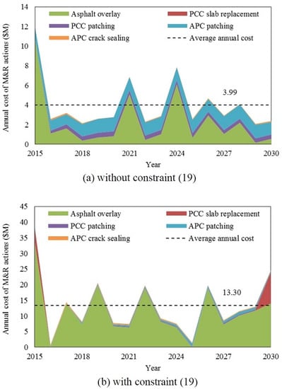
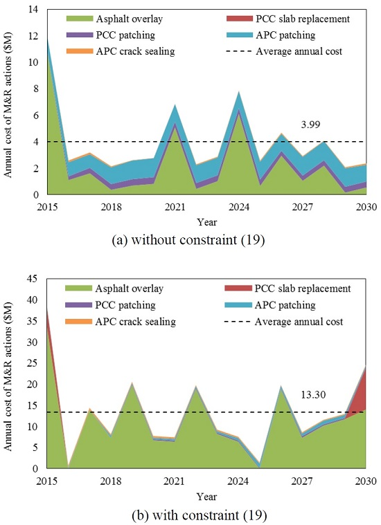
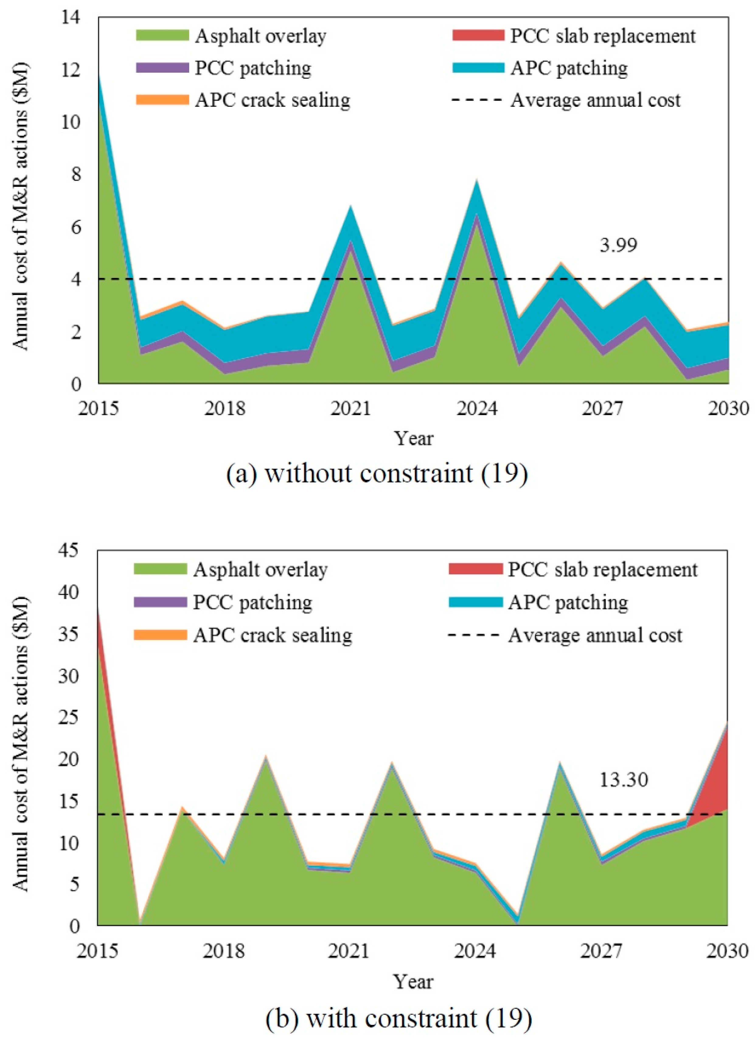
Figure 3a shows the distribution of annual M&R costs over the planning horizon without constraint (19). As mentioned earlier, the costs come from the simulation run of which the sum of simulated costs in each of the future years over the planning horizon plus the cost of the first year is the closest to the average over all simulation runs. The total M&R cost over 16 years is $63.9 million, or $4.0 million per year on average (indicated by the dashed line).

Table 5. Comparison of the proposed approach and PAVER in planning M&R activities at O’Hare.

	This Study	PAVER
Methodology for pavement condition forecast	Stochastic duration models that yield transition probabilities of pavement condition over time	Simple extrapolation of historic records that yield deterministic pavement condition forecast
Methodology for pavement M&R planning	Network-level optimization that account for interdependence of M&R activities among pavements	M&R activities determined based on pavement condition thresholds and prioritization rules
System-level performance requirement	Constraining the maximum fractions of pavements allowed in states 2 and 3	No constraints on the maximum fractions of pavements allowed in states 2 and 3
Planning horizon	2015–2030	2012–2021
Total M&R cost	$63.9 million	$58.0 million
Average M&R cost per year	$4.0 million	$5.8 million
Major actions considered (% of total M&R cost)	Asphalt overlay (55.60) PCC slab replacement (0.02)	Asphalt overlay (93.65) PCC slab replacement (4.12) PCC reconstruction (1.77)
Minor actions considered (% of total M&R cost)	APC patching (32.51) APC crack sealing (1.60) PCC patching (10.27)	APC patching (0.21) APC crack sealing (0.22) PCC patching (0.03)

provides a side-by-side comparison between the proposed approach and PAVER, in terms of methodology, system-level performance requirement, planning horizon considered, and M&R cost. Compared to the cost reported in the O’Hare Capital Improvement Plan [57] using PAVER, it is found that on average, the proposed approach will reduce annual M&R cost by $1.8 million. This is mainly due to a significant reduction in the major M&R costs and more extensive use of cheaper minor maintenance activities. It is worth noting again that, unlike the proposed approach, PAVER does not consider the requirement for the maximum fraction of pavement facilities in states 2 and 3 in each runway. As such, the results presented here appear superior to PAVER results not only in cost but in ensuring a high level of pavement performance.

Looking more closely into the results, fluctuations in annual costs are observed, which are due to the continuous deterioration of pavement conditions over time and the requirement for aggregate performance standards (constraint (17)). In fact, because the MILP formulation does not constrain the problem to be steady-state, fluctuations in annual costs is expected. A significant portion (nearly 20%) of the total M&R cost is attributed to the first year of the plan (2015) in order to improve the initial conditions of runway pavements (recall that more than 17% of the runways area is not in state 1 in 2015). Asphalt overlay and APC patching are the most contributing actions to the total cost with the respective shares of 55.6% and 32.5%, whereas PCC patching and APC crack sealing contribute to only 10.3% and 1.6% of the total cost. It is interesting to find that no PCC slab replacement is suggested over the planning horizon, probably because of its large unit cost.

Figure 3b depicts the distribution of annual M&R costs over the planning horizon when constraint (19) is considered to ensure that a major M&R action (asphalt overlay or slab replacement) is implemented on a whole runway—rather than on only part of it, should the major action be selected. Like Figure 3a, the costs come from the simulation run of which the sum of the simulated costs in each of the future years plus the cost of the first year is the closest to the average over all simulation runs. With this added constraint, the total M&R cost has increased significantly, to $212.8 million (note that the y-axis ranges are different in Figure 3a,b). This is not surprising, as adding constraint (19) eliminates the flexibility to perform major rehabilitation on only part of a runway. Among the simulated total cost, asphalt overlay accounts for the majority—86%. The cost shares of PCC slab replacement, PCC patching, APC patching, and APC crack sealing in the total are small, at 6.8%, 1.7%, 3.5%, and 2.0% respectively.

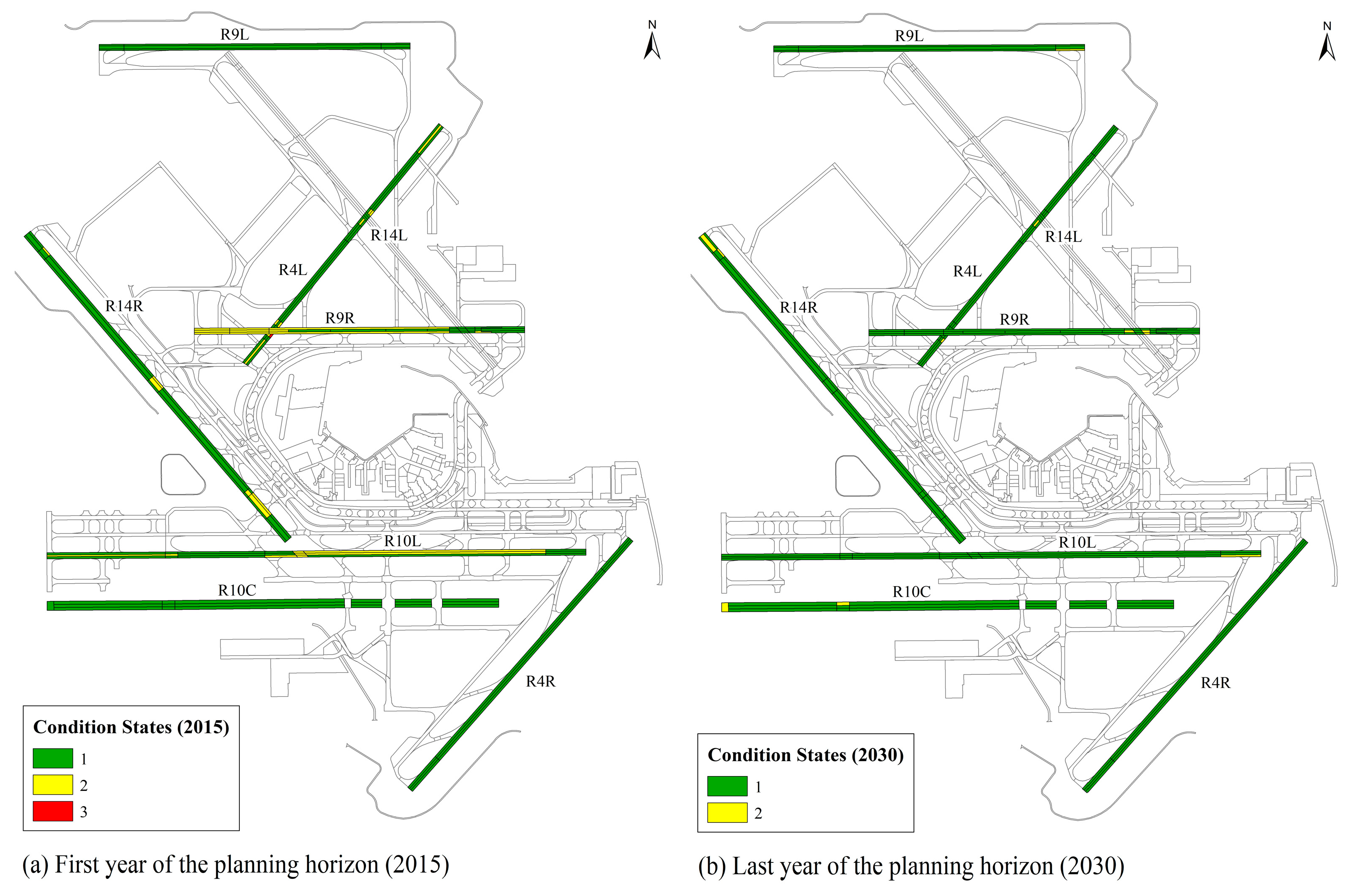
Figure 4 compares the condition states of the runway pavement network at the beginning of the planning horizon (Figure 4a) with the simulated condition states (see the M&R planning sub-section) at the end of the planning horizon (Figure 4b), without constraint (19). Same as Figure 3, Figure 4b is obtained from the simulation run that has the closest simulated total cost to the expected total cost in 2015. The maps show considerable improvement in the overall condition of the runway pavements, which is achieved at a significantly lower cost than the current practice.

5. Conclusions

This paper presents a modeling approach for planning M&R activities for a network of airport runway pavements. Decisions on M&R activities are guided by pavement condition forecasts based on stochastic duration models that capture the intrinsic uncertainty and dynamics in the pavement deterioration process and the impacts of exogenous factors. Using the pavement condition forecasts, a network optimization-based framework is developed which provides facility-specific M&R policies that minimize system-level M&R cost while accounting for the interdependence of M&R activities among pavement facilities over a planning horizon. The stochastic duration models and the network optimization-based framework are applied to studying runway pavement M&R at Chicago O’Hare International airport. The estimation results of the stochastic duration models show that pavement facilities surfaced with Portland cement concrete (PCC) have much slower deterioration rates than with asphalt overlay on PCC (i.e., APC). Past minor M&R activities were effective in slowing down pavement deterioration. Pavement facilities located on the keel of runways have, in some cases, higher deterioration rates than outband facilities due to heavier aircraft traffic loading. Compared to the state-of-the-practice, implementing the network optimization-based M&R planning framework can lead to much reduced M&R cost, meanwhile achieving a high-performance level for the runway pavement network.

This research makes a first attempt to demonstrate how a mathematical modeling approach that is more rigorous than the state-of-the-practice can help improve airport pavement management practice. Future research may be considered in the following directions. First, it would be helpful to improve the stochastic duration models with deeper “airport operation” inputs, which may generalize the results of the case study presented in the paper. Particularly, in the paper the effect of aircraft traffic loading on pavement deterioration is modeled by distinguishing between keel and outband facilities which bear significantly different aircraft traffic loadings, rather than based on aircraft traffic data due to data unavailability. Provided that such data become available in the future, further work can incorporate information on runway use by aircraft in the stochastic duration models. Second, additional efforts can be directed to collecting and incorporating temperature information into the stochastic duration models to capture the effect on pavement deterioration of low temperature cracking during winter. To use the models for pavement condition forecast, future years’ winter temperature over the planning horizon would be needed. Third, the current model could be improved to consider simultaneous implementation of major M&R actions on connection facilities in the present year as well as future years each time when the optimization is solved. One idea is to combine the current framework with approximate dynamic programming.

References

- Airport Improvement Program (AIP) Grant Data. Available online: https://www.faa.gov/airports/aip/grantapportion_data/ (accessed on 1 November 2018).
- Gendreau, M.; Soriano, P. Airport pavement management systems: An appraisal of existing methodologies. Transp. Res. Part A.: Policy Pract. 1998, 32, 197–214. [Google Scholar] [CrossRef]
- Shahin, M.Y. Pavement Management for Airports, Roads, and Parking Lots; Springer: New York, NY, USA, 2005. [Google Scholar]
- ACRP Common Airport Pavement Maintenance Practices: A Synthesis of Airport Practice. Available online: http://dot.ca.gov/hq/planning/aeronaut/documents/acrp/acrp_syn_022.pdf (accessed on 1 November 2018).
- Mishalani, R.G.; Madanat, S. Computation of infrastructure transition probabilities using stochastic duration models. J. Infrastruct. Syst. 2002, 8, 139–148. [Google Scholar] [CrossRef]
- Kuhn, K.D.; Madanat, S. Model uncertainty and the management of a system of infrastructure facilities. Transp. Res. Part C Emerg. Technol. 2005, 13, 391–404. [Google Scholar] [CrossRef] [Green Version]
- Madanat, S.; Bulusu, S.; Mahmoud, A. Estimation of infrastructure distress initiation and progression models. J. Infrastruct. Syst. 1995, 1, 146–150. [Google Scholar] [CrossRef]
- Madanat, S.; Wan Hashim, W.I. Poisson regression models of infrastructure transition probabilities. J. Transp. Eng. 1995, 121, 267–272. [Google Scholar] [CrossRef]
- Guillaumot, V.M.; Durango, P.L.; Madanat, S. Adaptive optimization of infrastructure maintenance and inspection decisions under performance model uncertainty. J. Infrastruct. Syst. 2003, 9, 133–139. [Google Scholar] [CrossRef]
- Golabi, K.; Kulkarni, R.B.; Way, G.B. A statewide pavement management system. Interfaces 1982, 12, 5–21. [Google Scholar] [CrossRef]
- Smilowitz, K.; Madanat, S. Optimal inspection and maintenance policies for infrastructure networks. Comput.-Aided Civ. Infrastruct. Eng. 2000, 15, 5–13. [Google Scholar] [CrossRef]
- Yeo, H.; Yoon, Y.; Madanat, S. Algorithms for bottom-up maintenance optimisation for heterogeneous infrastructure systems. Struct. Infrastruct. Eng. 2013, 9, 317–328. [Google Scholar] [CrossRef]
- Furuya, A.; Madanat, S. Accounting for network effects in railway asset management. J. Transp. Eng. 2013, 139, 92–100. [Google Scholar] [CrossRef]
- Camahan, J.V.; Davis, W.J.; Shahin, M.Y.; Keane, P.L.; Wu, M.I. Optimal maintenance decisions for pavement management. J. Transp. Eng. 1987, 113, 554–572. [Google Scholar] [CrossRef]
- Carnahan, J.V. Analytical framework for optimizing pavement maintenance. J. Transp. Eng. 1988, 114, 307–322. [Google Scholar] [CrossRef]
- Feighan, K.; Shahin, M.; Sinha, K.; White, T. Application of dynamic programming and other mathematical techniques to pavement management systems. Transp. Res. Rec. J. Transp. Res. Board 1988, 1200, 90–98. [Google Scholar]
- Harper, W.; Lam, J.; al-Salloum, A.; al-Sayyari, S.; al-Theneyan, S.; Ilves, G.; Majidzadeh, K. Stochastic optimization subsystem of a network-level bridge management system. Transp. Res. Rec. J. Transp. Res. Board 1990, 1268, 68–74. [Google Scholar]
- Gopal, S.; Majidzadeh, K. Application of Markov decision process to level-of-service-based maintenance systems. Transp. Res. Rec. J. Transp. Res. Board 1991, 1304, 12–18. [Google Scholar]
- Mayet, J.; Madanat, S. Incorporation of seismic considerations in bridge management systems. Comput.-Aided Civ. Infrastruct. Eng. 2002, 17, 185–193. [Google Scholar] [CrossRef]
- Lee, J.; Madanat, S. Jointly optimal policies for pavement maintenance, resurfacing and reconstruction. EURO J. Transp. Logist. 2015, 4, 75–95. [Google Scholar] [CrossRef]
- Durango, P.L.; Sarutipand, P. Capturing interdependencies and heterogeneity in the management of multifacility transportation infrastructure systems. J. Infrastruct. Syst. 2007, 13, 115–123. [Google Scholar] [CrossRef]
- Ouyang, Y. Pavement resurfacing planning for highway networks: Parametric policy iteration approach. J. Infrastruct. Syst. 2007, 13, 65–71. [Google Scholar] [CrossRef]
- Zou, B.; Madanat, S. Incorporating delay effects into airport runway pavement management systems. J. Infrastruct. Syst. 2012, 18, 183–193. [Google Scholar] [CrossRef]
- Robelin, C.; Madanat, S. Reliability-based system-level optimization of bridge maintenance and replacement decisions. Transp. Sci. 2008, 42, 508–513. [Google Scholar] [CrossRef]
- Chan, W.T.; Fwa, T.F.; Tan, C.Y. Road-maintenance planning using genetic algorithms I: Formulation. J. Transp. Eng. 1994, 120, 693–709. [Google Scholar] [CrossRef]
- Ng, M.; Lin, D.Y.; Waller, S.T. Optimal long-term infrastructure maintenance planning accounting for traffic dynamics. Comput.-Aided Civ. Infrastruct. Eng. 2009, 24, 459–469. [Google Scholar] [CrossRef]
- Medury, A.; Madanat, S. Simultaneous network optimization approach for pavement management systems. J. Infrastruct. Syst. 2013, 20, 04014010. [Google Scholar] [CrossRef]
- Nazari, F.; Noruzoliaee, M.; Zou, B.; Mohammadian, A. Optimal facility-specific inspection and maintenance decisions under measurement uncertainty: Unifying framework. J. Infrastruct. Syst. 2017, 23, 04017036. [Google Scholar] [CrossRef]
- Chan, P.; Oppermann, M.; Wu, S. North Carolina’s experience in development of pavement performance prediction and modeling. Transp. Res. Rec. J. Transp. Res. Board 1997, 1592, 80–88. [Google Scholar] [CrossRef]
- Jiang, Y.; Saito, M.; Sinha, K. Bridge performance prediction model using the Markov chain. Transp. Res. Rec. J. Transp. Res. Board 1988, 1180, 25–32. [Google Scholar]
- Ortiz-García, J.J.; Costello, S.B.; Snaith, M.S. Derivation of transition probability matrices for pavement deterioration modeling. J. Transp. Eng. 2006, 132, 141–161. [Google Scholar]
- Madanat, S.; Mishalani, R.; Wan Hashim, W.I. Estimation of infrastructure transition probabilities from condition rating data. J. Infrastruct. Syst. 1995, 1, 120–125. [Google Scholar] [CrossRef]
- Madanat, S.; Karlaftis, M.G.; McCarthy, P.S. Probabilistic infrastructure deterioration models with panel data. J. Infrastruct. Syst. 1997, 3, 4–9. [Google Scholar] [CrossRef]
- Anastasopoulos, P.C.; Labi, S.; Karlaftis, M.G.; Mannering, F.L. Exploratory state-level empirical assessment of pavement performance. J. Infrastruct. Syst. 2011, 17, 200–215. [Google Scholar] [CrossRef]
- Prozzi, J.A.; Madanat, S. Using duration models to analyze experimental pavement failure data. Transp. Res. Rec. J. Transp. Res. Board 2000, 1699, 87–94. [Google Scholar] [CrossRef]
- Mauch, M.; Madanat, S. Semiparametric hazard rate models of reinforced concrete bridge deck deterioration. J. Infrastruct. Syst. 2001, 7, 49–57. [Google Scholar] [CrossRef]
- Nakat, Z.S.; Madanat, S. Stochastic duration modeling of pavement overlay crack initiation. J. Infrastruct. Syst. 2008, 14, 185–192. [Google Scholar]
- Hong, F.; Prozzi, J.A. Estimation of pavement performance deterioration using Bayesian approach. J. Infrastruct. Syst. 2006, 12, 77–86. [Google Scholar] [CrossRef]
- Straub, D. Stochastic modeling of deterioration processes through dynamic Bayesian networks. J. Eng. Mech. 2009, 135, 1089–1099. [Google Scholar]
- Walgama, N.K.; Zhang, T.; Dwight, R. Calibrating Markov chain–based deterioration models for predicting future conditions of railway bridge elements. J. Bridge Eng. 2015, 20, 04014060. [Google Scholar]
- Roberts, C.A.; Attoh-Okine, N.O. A Comparative analysis of two artificial neural networks using pavement performance prediction. Comput.-Aided Civ. Infrastruct. Eng. 1998, 13, 339–348. [Google Scholar] [CrossRef]
- Bianchini, A.; Bandini, P. Prediction of pavement performance through neuro-fuzzy reasoning. Comput.-Aided Civ. Infrastruct. Eng. 2010, 25, 39–54. [Google Scholar] [CrossRef]
- Butler, B.; Carmichael, R., III; Flanagan, P. Impact of Pavement Maintenance on Damage Rate; Federal Highway Administration: Washington, DC, USA, 1985. [Google Scholar]
- Madanat, S.; Mishalani, R. Selectivity bias in modeling highway pavement maintenance effectiveness. J. Infrastruct. Syst. 1998, 4, 134–137. [Google Scholar] [CrossRef]
- Ben-Akiva, M.; Ramaswamy, R. An approach for predicting latent infrastructure facility deterioration. Transp. Sci. 1993, 27, 174–193. [Google Scholar] [CrossRef]
- Mohamad, D.; Sinha, K.; McCarthy, P. Relationship between pavement performance and routine maintenance: Mixed Logit approach. Transp. Res. Rec. J. Transp. Res. Board 1997, 1597, 16–21. [Google Scholar] [CrossRef]
- Chu, C.; Durango-Cohen, P.L. Incorporating maintenance effectiveness in the estimation of dynamic infrastructure performance models. Comput.-Aided Civ. Infrastruct. Eng. 2008, 23, 174–188. [Google Scholar] [CrossRef]
- Chu, C.; Durango-Cohen, P.L. Estimation of dynamic performance models for transportation infrastructure using panel data. Transp. Res. Part B 2008, 42, 57–81. [Google Scholar] [CrossRef]
- Chu, J.C. Condition-dependent maintenance effectiveness in dynamic performance models for transportation infrastructure. J. Infrastruct. Syst. 2013, 19, 85–98. [Google Scholar] [CrossRef]
- Greene, W. Econometric Analysis; Prentice Hall: Englewood Cliffs, NJ, USA, 2012. [Google Scholar]
- Ouyang, Y.; Madanat, S. An analytical solution for the finite-horizon pavement resurfacing planning problem. Transp. Res. Part B 2006, 40, 767–778. [Google Scholar] [CrossRef]
- Ouyang, Y.; Madanat, S. Optimal scheduling of rehabilitation activities for multiple pavement facilities: Exact and approximate solutions. Transp. Res. Part A Policy Pract. 2004, 38, 347–365. [Google Scholar] [CrossRef]
- Gu, W.; Ouyang, Y.; Madanat, S. Joint optimization of pavement maintenance and resurfacing planning. Transp. Res. Part B 2012, 46, 511–519. [Google Scholar] [CrossRef]
- Medury, A.; Madanat, S. Incorporating network considerations into pavement management systems: A case for approximate dynamic programming. Transp. Res. Part C Emerg. Technol. 2013, 33, 134–150. [Google Scholar] [CrossRef]
- Rubinstein, R.; Kroese, D. Simulation and the Monte Carlo Method; John Wiley & Sons: New York, NY, USA, 2011. [Google Scholar]
- Schwartz, G. Estimating the dimension of a model. Ann. Stat. 1978, 6, 461–464. [Google Scholar] [CrossRef]
- Chicago Department of Aviation. 10-Year Capital Improvement Program (CIP) 2012–2021; Chicago Department of Aviation: Chicago, IL, USA, 2011.
Figure 1.
Illustration of airport runway pavement facilities.
Figure 2.
Transition probabilities for pavement facilities in: (a)–(c) state 1; and (d,e) state 2.
Figure 3.
Annual M&R costs without (a) and with constraint (19) (b).
Figure 4.
Condition states of runway pavements at Chicago O’Hare airport. (a) First year of the planning horizon (2015). (b) Last year of the planning horizon (2030).