Stability Assessment of Earth Retaining Structures under Static and Seismic Conditions

Abstract

An accurate estimation of static and seismic earth pressures is extremely important in geotechnical design. The conventional Coulomb’s approach and Mononobe-Okabe’s approach have been widely used in engineering practice. However, the latter approach provides the linear distribution of seismic earth pressure behind a retaining wall in an approximate way. Therefore, the pseudo-dynamic method can be used to compute the distribution of seismic active earth pressure in a more realistic manner. The effect of wall and soil inertia must be considered for the design of a retaining wall under seismic conditions. The method proposed considers the propagation of shear and primary waves through the backfill soil and the retaining wall due to seismic excitation. The crude estimate of finding the approximate seismic acceleration makes the pseudo-static approach often unreliable to adopt in the stability assessment of retaining walls. The predictions of the active earth pressure using Coulomb theory are not consistent with the laboratory results to the development of arching in the backfill soil. A new method is proposed to compute the active earth pressure acting on the backface of a rigid retaining wall undergoing horizontal translation. The predictions of the proposed method are verified against results of laboratory tests as well as the results from other methods proposed in the past.

1. Introduction

Study of dynamic active earth pressure is essential for the safe design of a retaining wall in the seismic zone. A pioneering theory of dynamic lateral earth pressure based on the pseudo-static method of analysis commonly known as the Mononobe-Okabe method is commonly adopted in practice. The simplicity of the method lies in the basic assumption of a planar rupture surface along with seismic forces that are pseudo-static in nature. The seismic earth pressure is estimated from the force equilibrium of the failure wedge. Many researchers employed different theories to determine the earth pressure under static and seismic conditions. These different methodologies are listed below:

• Pseudo-static limit equilibrium analysis [1,2,3,4,5,6,7,8,9,10,11,12,13].
• Pseudo-static limit analysis [14,15].
• Soil-structure interaction based method [16,17,18,19,20].
• Displacement based earth pressure theories [21,22,23,24,25].
• Pseudo-dynamic limit equilibrium analysis [26,27,28,29,30,31].
• Arch action based theories [32,33,34,35,36].

In the above seismic studies, except the pseudo-dynamic method, the seismic forces are assumed to be pseudo-static in nature. However, the pseudo-static method does not consider the effect of time and seismic waves. Nakamura [37] conducted a series of centrifuge model tests to re-examine the assumptions of the Mononobe–Okabe theory of gravity retaining walls. Based on these experimental results, Nakamura [37] concluded that the maximum values of wall inertia and dynamic earth pressure do not occur simultaneously. Athanasopoulos-Zekkos et al. [38] numerically validated the experimental results reported by Nakamura [37]. Based on the results of centrifuge experiments on cantilever retaining walls, Al-Atik and Sitar [39] suggested that design of retaining walls for maximum dynamic earth pressure increment and maximum wall inertia is overly conservative.

A closed-form solution using plasticity theorem is proposed by Mylonakis et al. [14] for gravity retaining walls under seismic conditions. Li et al. [15] determined the yield acceleration for translation failure of gravity retaining walls based on the upper bound theorem of limit analysis. Authors have concluded that the wall roughness has a remarkable influence on the yield acceleration.

Veletsos and Younan [16] developed an analytical approach for evaluating the magnitude and distribution of the dynamic displacements, pressures, and forces induced by horizontal ground shaking in walls that are both flexible and elastically constrained against rotation at their base. The soil is considered to act as a uniform, infinitely extended visco-elastic stratum. The base of the wall and the soil stratum are considered to be excited by a space-invariant horizontal motion, assuming an equivalent force-excited system. Psarropoulos et al. [18] numerically validated (using the finite element method) the solution proposed by Veletsos and Younan [16]. Jung et al. [19] expanded the analytical solution by Veletsos and Younan [16] by including the horizontal translation of the wall. Jung et al. [19] correctly pointed out that these assumptions introduce very important limitations to the applicability of the solution to the design of retaining structures. However, a close-form solution provides a rational framework where the effects of different parameters can be analysed.

Saran et al. [23] discretized the continuous interaction of the backfill using the concept of soil modulus as closely spaced independent elastic springs. One end of the spring is fixed, and the other end is attached to the back of a vertical retaining wall. Authors have considered three different types of wall movement: translation, rotation about the bottom, and rotation about the top of the wall. The active earth pressure coefficient and earth pressure distribution is proposed. Saran et al. [24] further extended the solution for different backfill and wall inclination angle. The mobilisation of friction angle between the wall and backfill is also studied.

Tizando and Rodríguez-Roa [40] carried out a series of 2D dynamic finite-element analyses to study the behaviour of gravity retaining walls on normally consolidated granular soils. Authors applied Chilean strong motion records at the bed rock level of the proposed numerical model.

Steedman and Zeng [26] proposed a simple pseudo-dynamic analysis to determine seismic active earth thrust on a retaining wall that incorporates phase difference and assumes amplification effects in the dry cohesionless backfill subjected only to horizontal acceleration that varies along the face of the wall. Choudhury and Nimbalkar [27] modified this methodology to incorporate the effect of vertically propagating primary waves on the seismic active thrust. Ghosh [28] proposed the seismic active thrust on an inclined retaining wall using the pseudo-dynamic approach. Choudhury and Ahmad [7,8] extended the work of Choudhury and Nimbalkar [27] and proposed closed-form solutions for the seismic stability of waterfront retaining walls. Kolathayar and Ghosh [29] studied the seismic active thrust behind a rigid cantilever retaining wall with bilinear backface using the same approach. Ghanbari and Ahmadabadi [30] proposed a horizontal slice method using the pseudo-dynamic approach to obtain the seismic active thrust on an inclined retaining wall. Ghosh and Sharma [31] studied the effect of backfill inclination on the seismic active thrust.

Using this methodology, the sliding stability of a retaining wall is studied by Baziar et al. [41]. Baziar et al. [41] proposed a combined dynamic factor that considers the effect of seismic active thrust and inertia forces in the wall. The safe weight of the retaining wall under the seismic condition can be obtained by simply multiplying this factor with the weight of the wall required for equilibrium against sliding under the static condition. Choudhury and Nimbalkar [42] computed the rotational displacement of the vertical gravity retaining wall using the rotating block method (Zeng and Steedman [43]). The seismic inertia forces are computed using the pseudo-dynamic method. Pain et al. [44] proposed to update the location of the rotating wall and its influence on the directions of external forces during each time increment of the calculation of rotational displacement. The analysis also shows that the assumption of Zeng and Steedman [43] is valid only for very small values of rotational displacement (rotational displacement < 1°). Authors concluded that the rotational displacement does not only depend on the properties of the backfill, however it also depends on the characteristics of the input motion, wall geometry, and the properties of the wall material. Four different modes of failure, viz. sliding, overturning, eccentricity, and bearing capacity, of foundation soil was considered by Basha and Babu [45] for the optimum design of bridge abutments when subjected to earthquake loading. Authors have used the pseudo-dynamic approach to compute the seismic inertia forces.

Despite its various applications, the pseudo-dynamic method only considers the vertically upward propagating sinusoidal waves. It does not consider the interaction of upward propagating waves and the waves reflected from the free ground surface. The pseudo-dynamic method originally proposed by Steedman and Zeng [26] and subsequently modified by Choudhury and co-workers does not consider the effect of damping, and the amplification of acceleration towards the ground surface is unbound. An appropriate value of amplification factor needs to be assumed in the analysis. Bellezza [46,47] solved the 1D wave equation, assuming the dry homogeneous cohesionless backfill as Kelvin-Voigt solid to derive the acceleration distribution within the retained fill. The differential equation is solved using boundary conditions and the author showed that the acceleration distribution is non-linear in nature. Bellezza [46] highlighted the drawbacks of the original pseudo-dynamic method and subsequently proposed an alternative solution that addresses some of the stated drawbacks. However, none of these methods consider the interaction between the wall and the backfill soil. In the proposed method, the wall–soil interaction under the seismic condition addressing the stated drawbacks is explored considering horizontal as well as vertical inertia force. The solution is valid for a harmonic base excitation that satisfies the boundary condition. These assumptions introduce very important limitations to the applicability of the solution to the design of retaining structures, however a close-form solution has the advantage of providing a rational framework where the effects of different parameters can be analysed. The main objective of the present study lies in this route.

In the pioneer study by Harop-Williams [48], soil arching is found to influence the nonlinear distribution of the active earth pressure acting on the rigid walls. This is in contrast with the assumption made by Coulomb (1776) and Rankine (1857) theories. A method for calculating the active earth pressures assuming Coulomb slip is proposed (Wang [49]). However, none of these studies considered the stress trajectory caused by the soil arching effect, a common phenomenon that is prevalent in geotechnical engineering practice.

In the recent past, methods for the determination of active earth pressure considering the soil arching effects were proposed (Paik & Salgado [33], Li & Wang [50]). However, these methods are limited to non-cohesive soils. Considering this, a simplified method for calculating the active earth pressure acting on a rigid retaining wall undergoing translation is proposed in this study.

2. Seismic Active Thrust Using the Pseudo-Dynamic Method

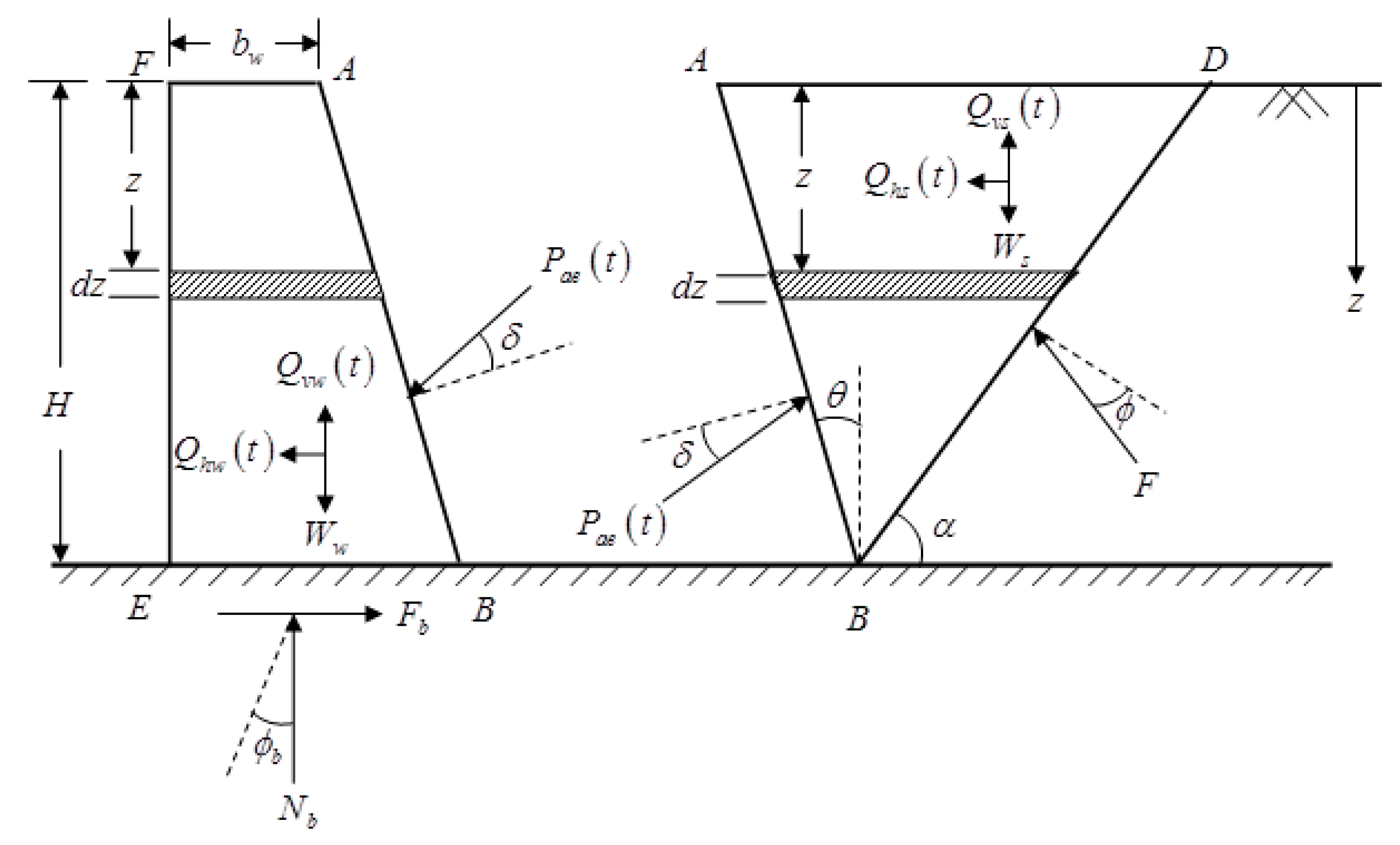
A fixed base inclined rigid retaining wall of height H is considered as shown in Figure 1. The wall supports a cohesionless backfill material with horizontal ground. The shear wave and primary wave are assumed to act within the soil media due to earthquake loading. The ratio, V_p/V_s = 1.87 is assumed to be valid for the most geological materials. The period of lateral shaking is defined as T = 2π/ω, where ω is the angular frequency. A planer rupture surface inclined at an angle, α with the horizontal is considered.

The base of the wall is subjected to harmonic horizontal seismic acceleration of amplitude k_hg, and harmonic vertical seismic acceleration of amplitude k_vg, where g is the acceleration due to gravity. The acceleration at any depth z and time t below the top of the wall can be expressed as,

$$a_{hs}(z,\mathrm{t})={\mathrm{k}}_{\mathrm{h}}\sin \left[t-\frac{H-z}{V_s}\right]$$

(1)

$$a_{vs}(z,\mathrm{t})=k_{\mathrm{v}}\sin \left[t-\frac{H-z}{V_p}\right]$$

(2)

The mass of an elemental wedge at depth z is

$$m_s(z)=\frac{{\gamma }_b\left(H-z\right)\left[\tan \theta +\cot \alpha \right]}{g}dz$$

(3)

where γ_b is the unit weight of the backfill. The total horizontal and vertical inertia forces acting within the failure zone ABD is expressed as:

$$Q_{hs}\left(t\right)={\displaystyle \underset{0}{\overset{H}{\int }}{m}_s\left(z\right)a_{hs}\left(z,t\right)}$$

(4)

$$Q_{vs}\left(t\right)={\displaystyle \underset{0}{\overset{H}{\int }}{m}_s\left(z\right)a_{vs}\left(z,t\right)}$$

(5)

The total (static + seismic) active thrust, P_ae(t) is obtained by resolving the forces on the wedge. Considering the equilibrium of the forces and hence P_ae(t) is expressed as follows,

$$P_{ae}\left(t\right)=\frac{W_s\sin \left(\alpha -\varphi \right)+Q_{hs}\left(t\right)\cos \left(\alpha -\varphi \right)-Q_{vs}\left(t\right)\sin \left(\alpha -\varphi \right)}{\cos \left(\varphi +\delta +\theta -\alpha \right)}$$

(6)

where the weight of the soil wedge ABD; $W_s=0.5{\gamma }_b{H}^2\left(\tan \theta +\cot \alpha \right)$. Hence, the seismic active earth pressure coefficient is obtained as

$$K_{ae}\left(t\right)=\frac{2P_{ae}\left(t\right)}{\gamma H^2}$$

(7)

3. Seismic Active Thrust Using the Modified Pseudo-Dynamic Method

Yuan et al. [51] proposed the equation of motion of stress waves travelling through visco-elastic medium. In the vector form, the equation of motion is written as:

$$\rho \frac{{\partial }^2\overline{u}}{\partial t^2}=\left\{\left(\lambda +G\right)+\left({\eta }_l+{\eta }_s\right)\frac{\partial }{\partial t}\right\}grad\left(\kappa \right)+\left(G+{\eta }_s\frac{\partial }{\partial t}\right){\nabla }^2\overline{u}$$

(8)

where ρ = density; λ = Lamé constant; G = Shear modulus; η_l and η_s = Viscosities; $\overline{u}$ = Displacement vector and κ = div ($\overline{u}$). The solution of a plane wave propagating vertically in a Kelvin-Voigt homogeneous medium for the computation of earth pressure under seismic condition is obtained. The proposed simplified form of Equation (1) is given below

$$\rho \frac{{\partial }^2{u}_h}{\partial t^2}=G\frac{{\partial }^2{u}_h}{\partial z^2}+{\eta }_s\frac{{\partial }^3{u}_h}{\partial t\partial z^2}$$

(9)

$$\rho \frac{{\partial }^2{u}_v}{\partial t^2}=\left(\lambda +2G\right)\frac{{\partial }^2{u}_v}{\partial z^2}+\left({\eta }_l+2{\eta }_s\right)\frac{{\partial }^3{u}_v}{\partial t\partial z^2}$$

(10)

Kelvin–Voigt solid is used to model the backfill soil. The stress-strain relationship of Kelvin-Voigt is given below:

$$\tau ={\gamma }_{s}G+{\eta }_s\frac{\partial {\gamma }_s}{\partial t}$$

(11)

where τ = shear stress; γ_s = shear strain; η_s = viscosity, G = shear modulus. For a horizontal harmonic base shaking of angular frequency ω; ${\eta }_s$ = $\frac{2G\xi }{\omega }$ where $\xi$ = damping ratio. Equation (9) is solved for a harmonic horizontal shaking. At the ground surface (z = 0), shear stress is zero. Assuming a base displacement $u_{hb}=u_{h0}\cos \left(\omega t\right)$, the horizontal displacement is obtained as

$$u_h\left(z,t\right)=\frac{u_{h0}}{C_s{}^2+S_s{}^2}\left[\left(C_s{C}_{sz}+S_s{S}_{sz}\right)\cos \left(\omega t\right)+\left(S_s{C}_{sz}-C_s{S}_{sz}\right)\sin \left(\omega t\right)\right]$$

(12)

where, C_s, S_s, C_sz, and S_sz depend on normalized frequency (ωH/V_s) and damping ratio (ξ).

$$C_{sz}=\cos \left(\frac{y_{s1}z}{H}\right)\cosh \left(\frac{y_{s2}z}{H}\right)$$

(13a)

$$S_{sz}=-\sin \left(\frac{y_{s1}z}{H}\right)\sinh \left(\frac{y_{s2}z}{H}\right)$$

(13b)

$$C_s=\cos \left(y_{s1}\right)\cosh \left(y_{s2}\right)$$

(14a)

$$S_s=-\sin \left(y_{s1}\right)\sinh \left(y_{s2}\right)$$

(14b)

$$y_{s1}=\frac{\omega H}{V_s}\sqrt{\frac{\sqrt{1+4{\xi }^2}+1}{2\left(1+4{\xi }^2\right)}}$$

(15a)

$$y_{s2}=-\frac{\omega H}{V_s}\sqrt{\frac{\sqrt{1+4{\xi }^2}-1}{2\left(1+4{\xi }^2\right)}}$$

(15b)

The horizontal acceleration is obtained by differentiating Equation (12) twice with respect to time:

$$a_h\left(z,t\right)=\frac{k_{h}g}{C_s{}^2+S_s{}^2}\left[\left(C_s{C}_{sz}+S_s{S}_{sz}\right)\cos \left(\omega t\right)+\left(S_s{C}_{sz}-C_s{S}_{sz}\right)\sin \left(\omega t\right)\right]$$

(16)

where $k_{h}g=-{\omega }^2{u}_{h0}$; k_h = Horizontal seismic acceleration coefficient at the base.

Equation (10) is expressed in a form similar to Equation (9) provided that u_h, G, and η_s are replaced by u_v, E_c (= λ + 2G) and η_p = (η_l + 2η_s), respectively. Similarly, Equation (10) is solved for the case of harmonic vertical shaking. At the ground surface (z = 0), normal stress is zero. Assuming a base displacement $u_{vb}=u_{v0}\cos \left(\omega t\right)$, the vertical displacement is obtained as:

$$u_v\left(z,t\right)=\frac{u_{v0}}{C_p{}^2+S_p{}^2}\left[\left(C_p{C}_{pz}+S_{ps}{S}_{pz}\right)\cos \left(\omega t\right)+\left(S_p{C}_{pz}-C_p{S}_{pz}\right)\sin \left(\omega t\right)\right]$$

(17)

where C_p, S_p, C_pz, and S_pz depend on normalized frequency (ωH/V_p) and damping ratio (ξ).

$$C_{pz}=\cos \left(\frac{y_{p1}z}{H}\right)\cosh \left(\frac{y_{p2}z}{H}\right)$$

(18a)

$$S_{pz}=-\sin \left(\frac{y_{p1}z}{H}\right)\sinh \left(\frac{y_{p2}z}{H}\right)$$

(18b)

$$C_p=\cos \left(y_{p1}\right)\cosh \left(y_{p2}\right)$$

(19a)

$$S_p=-\sin \left(y_{p1}\right)\sinh \left(y_{p2}\right)$$

(19b)

$$y_{p1}=\frac{\omega H}{V_p}\sqrt{\frac{\sqrt{1+4{\xi }^2}+1}{2\left(1+4{\xi }^2\right)}}$$

(20a)

$$y_{p2}=-\frac{\omega H}{V_p}\sqrt{\frac{\sqrt{1+4{\xi }^2}-1}{2\left(1+4{\xi }^2\right)}}$$

(20b)

Vertical acceleration can be obtained by differentiating Equation (17) twice with respect to time:

$$a_v\left(z,t\right)=\frac{k_{v}g}{C_p{}^2+S_p{}^2}\left[\left(C_p{C}_{pz}+S_p{S}_{pz}\right)\cos \left(\omega t\right)+\left(S_p{C}_{pz}-C_p{S}_{pz}\right)\sin \left(\omega t\right)\right]$$

(21)

where $k_{v}g=-{\omega }^2{u}_{v0}$; k_v = Vertical seismic acceleration coefficient at the base. The total horizontal and vertical inertial forces acting within the active wedge ABD are obtained following the same procedure as described in the pseudo-dynamic method of analysis, however the only difference is that the expression of acceleration is used as given in Equations (17) and (21). The value of shear and primary wave velocity and damping ratio (ξ_s) of the backfill material should be used.

3.1. Stability of Rigid Retaining Wall Under Seismic Conditions Using the Modified Pseudo-Dynamic Method

First, the total horizontal and vertical inertial forces acting on the wall AFEB is computed

$$Q_{hw}\left(t\right)={\displaystyle \underset{0}{\overset{H}{\int }}{m}_w\left(z\right)a_{hw}\left(z,t\right)}$$

(22)

$$Q_{vw}\left(t\right)={\displaystyle \underset{0}{\overset{H}{\int }}{m}_w\left(z\right)a_{vw}\left(z,t\right)}$$

(23)

where the mass of a thin element dz of the wall AFEB at depth z is

$$m_w(z)=\frac{{\gamma }_w\left[b_w+z\tan \theta \right]}{g}dz$$

(24)

and a_hw(z,t) and a_vw(z,t) are obtained by putting the value of shear and primary wave velocity and damping ratio (ξ_w) of the wall material in Equations (17) and (21). Using D’Alembert’s principle for inertial forces acting on the wall as shown in Figure 1, the weight of the wall required for equilibrium against sliding under seismic conditions is obtained as:

$$W_w\left(t\right)=P_{ae}\left(t\right)\left[\frac{\cos \left(\delta +\theta \right)-\sin \left(\delta +\theta \right)\tan {\varphi }_b}{\tan {\varphi }_b}+\frac{Q_{hw}\left(t\right)+Q_{vw}\left(t\right)\tan {\varphi }_b}{P_{ae}\left(t\right)\tan {\varphi }_b}\right]$$

(25)

where ${\varphi }_b$ is the friction angle at the base of the wall.

$$W_w\left(t\right)=P_{ae}\left(t\right)C_{IE}\left(t\right)$$

(26)

where C_IE(t) is the dynamic wall inertia factor given by

$$C_{IE}\left(t\right)=\left[\frac{\cos \left(\delta +\theta \right)-\sin \left(\delta +\theta \right)\tan {\varphi }_b}{\tan {\varphi }_b}+\frac{Q_{hw}\left(t\right)+Q_{vw}\left(t\right)\tan {\varphi }_b}{P_{ae}\left(t\right)\tan {\varphi }_b}\right]$$

(27)

The relative importance of dynamic effects viz. (i) increased seismic active thrust on the wall due to modified pseudo-dynamic soil inertia forces on the sliding wedge and (ii) the increase in driving force due to time dependent inertia of the wall itself is evident by normalizing them with regard to the static values. Thus, the soil thrust factor, F_T is defined as

$$F_T=\frac{K_{ae}\left(t\right)}{K_a}$$

(28)

And wall inertia factor, F_I is defined as

$$F_I=\frac{C_{IE}\left(t\right)}{C_I}$$

(29)

where,

$$C_I=\frac{\cos \left(\delta +\theta \right)-\sin \left(\delta +\theta \right)\tan {\varphi }_b}{\tan {\varphi }_b}$$

(30)

The combined dynamic factor, F_W proposed for the design of the wall is defined as

$$F_W=F_T{F}_I=\frac{W_w\left(t\right)}{W_{w,static}}$$

(31)

where W_w,static is the weight of the wall required for equilibrium against sliding under static condition.

3.2. Results and Discussion

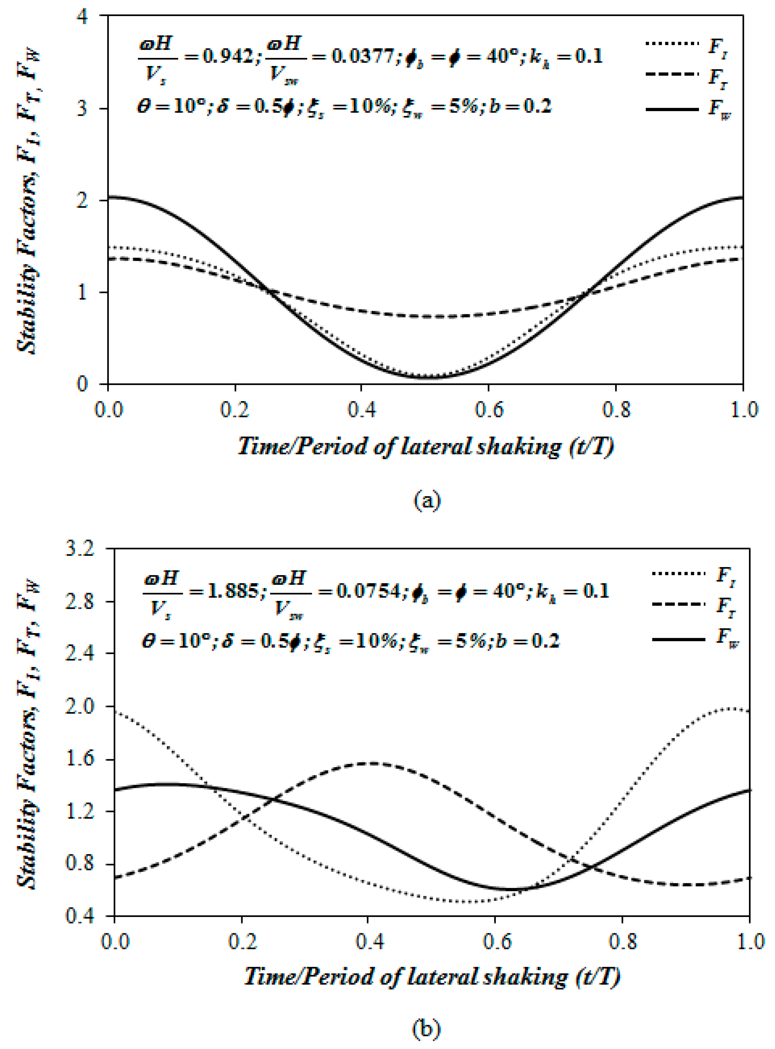
Pain et al. [52] optimized α and t simultaneously to maximize F_W. Figure 2a shows that the stability factors are in phase and they attain their maximum values almost at the same time of the instance at t/T = 0.5. Figure 2b shows the variation of the stability factors F_I, F_T, and F_W for the given input parameters. The maximum value of F_W is 1.41 and occurs at t/T = 0.081, whereas the maximum active thrust occurs at t/T = 0.402 and the value of F_W is 1.02. It is clear that when F_W has attained the maximum value, other two partial factors may not have attained their peak values.

Figure 3 shows the distribution of horizontal acceleration along the depth at the instant of maximum value of F_W for different sets of normalized frequencies (ωH/V_s and ωH/V_sw) keeping the other input parameters the same as in Figure 2a. The acceleration distribution along the depth is nonlinear in nature. It is worth mentioning that for the value of ωH/V_s = 1.885 and ωH/V_sw = 0.0754, the inertia force in the active wedge acts in the opposite direction to that mentioned in Figure 1, which in turn reduces the active thrust on the wall. On the contrary, the inertia force in the wall acts simultaneously in the direction shown in the Figure 1. The amplitude and phase of acceleration vary with depth in the modified pseudo-dynamic method (Pain et al. [52]). In the modified pseudo-dynamic method, the amplification of acceleration depends on the soil properties and no simplifying assumption of any amplification value is necessary. Seismic inertia forces are functions of normalized frequency (ωH/V) and damping ratio (ξ). At frequencies above the normalized fundamental frequency (ωH/V_s = π/2), part of the active wedge moves in one direction while another part moves in the opposite direction (See Figure 3 for ωH/V_s = 1.885). However, the active wedge moves in the same direction when ωH/V_s < π/2. This is one of the unique aspects of the modified pseudo-dynamic method.

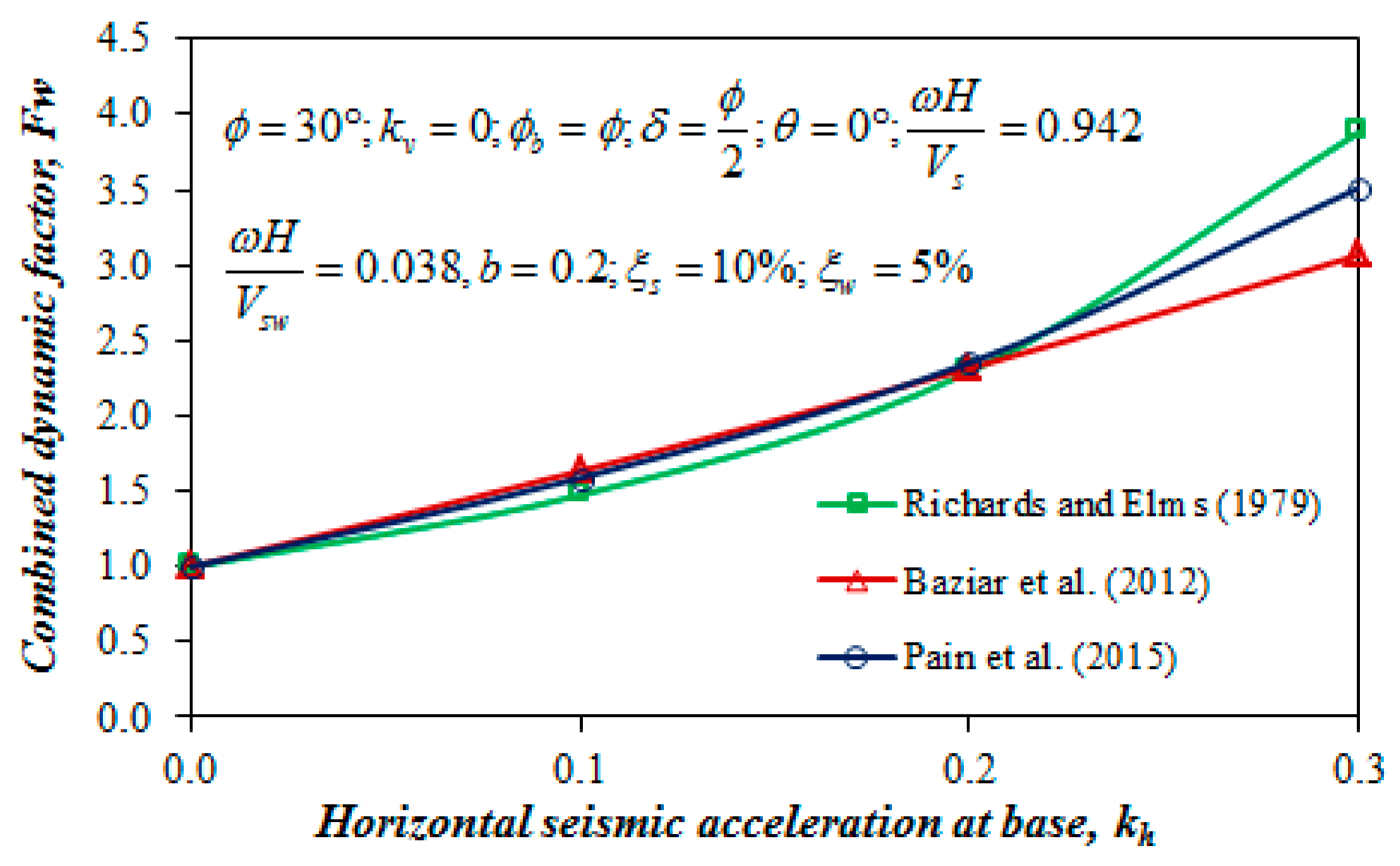
Figure 4 shows the comparison of the combined dynamic factor with the values reported by Richards and Elms [21], Baziar et al. [41], and Pain et al. [52]. Pain et al. [52] report that the wall inertia factor computed using the modified pseudo-dynamic method are lesser than those obtained using the pseudo-static method of Richards and Elms [21] and pseudo-dynamic method of Baziar et al. [41]. The soil thrust factor is found to be the highest for the modified pseudo-dynamic method. Pain et al. [52] attributed this difference to the amplification of acceleration towards the ground surface. Richards and Elms [21] and Baziar et al. [41] did not consider the increase in the soil thrust factor due to the amplification of acceleration. As is evident from Figure 4, the values obtained using the method of Richards and Elms [21] are highest when the horizontal seismic acceleration coefficient (k_h) exceeds 0.2. The values reported by Pain et al. [52] are higher than the values of Baziar et al. [41] for the given set of input parameters. This is attributed to the fact that the effect of amplification of acceleration is not considered by Baziar et al. [41]. This difference may change depending on the variation in input parameters.

4. Effect of Soil Arching on the Stability of Retaining Structures

The retaining wall is considered to be rigid and the backfill soil is considered to be cohesive. A planer failure surface is considered in accordance with previous studies (Choudhury & Ahmad [7,8]). The analysis of lateral active earth pressure in cohesive soils is carried out using the horizontal flat element method. In this method (Rao et al. [36]), the failure wedge is divided into a number of horizontal flat elements.

4.1. Analytical Model

Considering the effects of soil arching and wall-soil friction, a new coefficient of lateral active earth pressure (K_aw) is defined as:

$$K_{aw}=\frac{1+\frac{1-\sin \varphi }{1+\sin \varphi }{\cot }^2\left(\frac{1}{2}\arcsin \left(\frac{\sin \delta }{\sin \varphi }\right)-\frac{\delta }{2}\right)}{{\csc }^2\left(\frac{1}{2}\arcsin \left(\frac{\sin \delta }{\sin \varphi }\right)-\frac{\delta }{2}\right)-\frac{2\sin \varphi }{3(1+\sin \varphi )}}$$

(32)

From Equation (32), it is established that when the wall surface is smooth (i.e., δ = 0), $K_{aw}=K_a={\tan }^2(45°-\varphi /2)$, which coincides with Rankine’s active earth pressure coefficient. The lateral active earth pressure at the back of the wall is expressed as:

$${\sigma }_h=K_{aw}\left[\begin{array}{l}\left(q+\frac{\gamma H}{1+\chi }+\frac{c}{\tan \varphi }\right)\times \\ {\left(1-\frac{y}{H}\right)}^{-\chi }-\gamma \left(\frac{H-y}{1+\chi }\right)\end{array}\right]-\frac{c}{\tan \varphi }$$

(33)

If cracks do not appear in the backfill surface, integrating Equation (33) with respect to y, the active thrust is obtained:

$$E_h={\displaystyle \underset{0}{\overset{H}{\int }}{\sigma }_h\mathrm{d}y}=\xi \left(qH+\frac{\gamma H^2}{2}\right)-\left(1-\xi \right)\frac{cH}{\tan \varphi }$$

(34)

where

$$\xi =\frac{\sin \left(\lambda -\frac{\varphi +\delta }{2}\right)\cos \delta }{\cos \left(\lambda -\frac{\varphi +3\delta }{2}\right)\tan \left(\lambda +\frac{\varphi -\delta }{2}\right)}$$

(35)

From the analysis of Equations (34) and (35), it is observed that when the wall surface is smooth (i.e., δ = 0), $\xi =K_a={\tan }^2(45°-\phi /2)$ which coincides with the Rankine’s active earth pressure coefficient. The active thrust is also found to match to that computed by Rankine’s theory [1857]. If a crack appears at a given depth (H_c) within the backfill, the lateral earth pressure within this depth is assumed to be zero. By integrating Equation (33) with respect to y from H_c to H, the lateral active earth pressure force is obtained as given below:

$$E_h={\displaystyle \underset{H_c}{\overset{H}{\int }}{\sigma }_h\mathrm{d}y}=\xi \left(H-H_c\right)\left[q{\left(1-\frac{H_c}{H}\right)}^{-\chi }-\left(\frac{{\eta }_{c}c}{\tan \varphi }\right)+{\eta }_r\gamma \left(\frac{H-H_c}{1+\chi }\right)\right]$$

(36)

where

$${\eta }_c=\frac{1}{\xi }-{\left(1-\frac{H_c}{H}\right)}^{-\chi }$$

(37)

$${\eta }_r={\left(1-\frac{H_c}{H}\right)}^{-1-\chi }-\left(\frac{1-\chi }{2}\right)$$

(38)

4.2. Results and Discussion

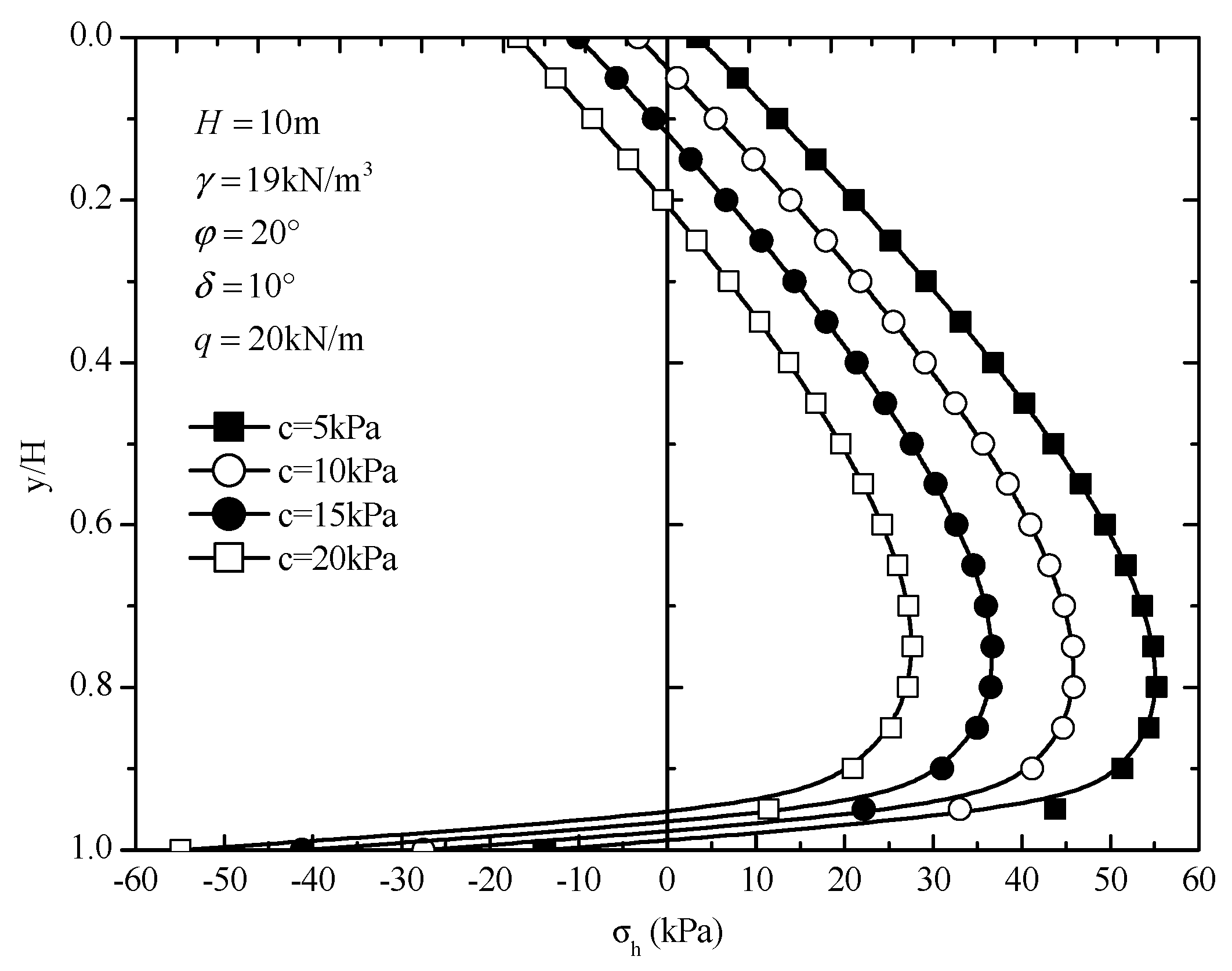
Figure 5 shows the lateral active earth pressure distribution along the normalised height (y/H) of a translating rigid wall with cohesive backfill soil for various values of soil cohesion. It is evident that the lateral active earth pressure distribution along the rigid wall exhibits a nonlinear shape for the entire range of soil cohesion considered in this study.

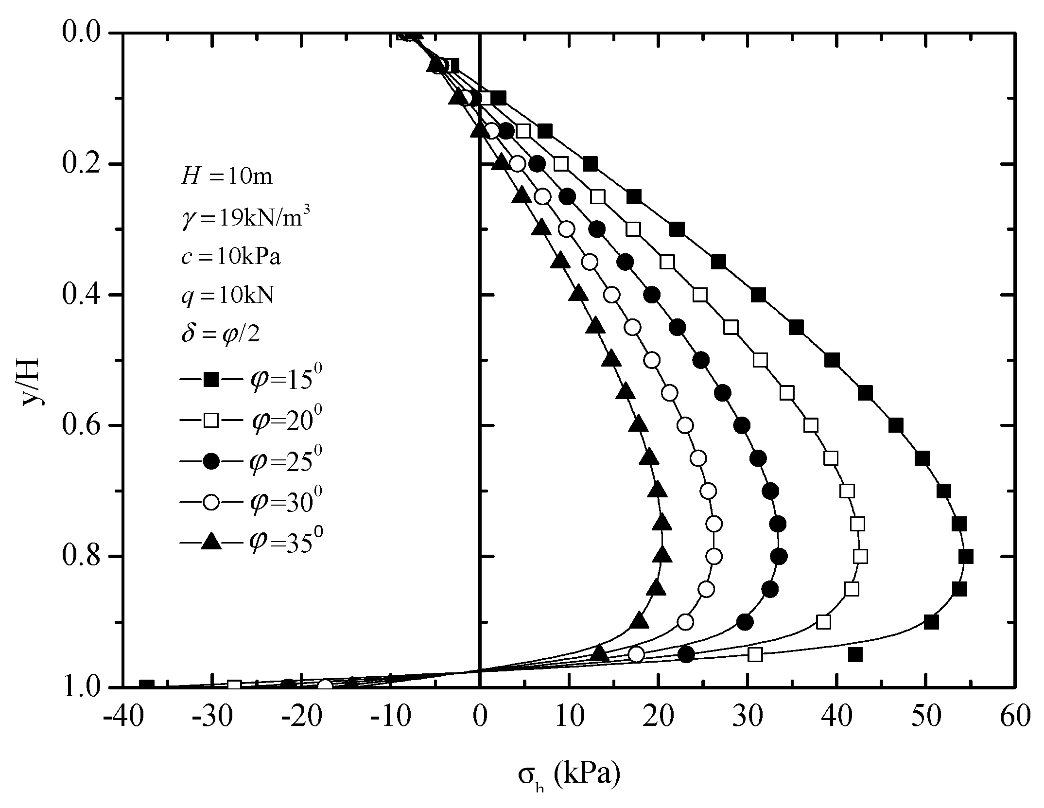
The lateral active earth pressure decreases significantly with the increase of the soil cohesion c., while it is interesting to note that the normalised height of the point of application of active thrust increases marginally. In addition, the depth of the tension crack from the surface of the cohesive backfill soil is developed significantly, which is attributed to the increase in soil cohesion. Figure 6 shows the lateral active earth pressure distribution along the normalised height (y/H) of a translating rigid wall with cohesive backfill soil for various friction angles (φ). It is apparent that the lateral active earth pressure decreases significantly with the increase in internal friction angle of cohesive soil, while the shape of the lateral active earth pressure distribution remains unchanged. The normalised height of the point of application of the active thrust from the base of the wall increases marginally. The depth of tension crack from the surface of the cohesive soil increases significantly as φ increases.

4.3. Comparison with Other Studies

In order to check the applicability of the proposed formulations, the predictions from the derived equation are compared with experimental results reported by Tsagareli [53], where the distribution of the active earth pressures acting on the translating rigid retaining wall with the height of 4 m are measured. Figure 7 shows the comparison of the non-dimensional distributions of the active earth pressure with other studies (Coulomb 1776, Rankine 1857). It is evident that the results obtained using the proposed equation are in good agreement with the measured values. The proposed method is successful in capturing the salient feature of non-linear distribution of active earth pressures, which cannot be predicted by using the existing Coulomb’s (1776) and Rankine’s theories (1857).

5. Conclusions

In pseudo-dynamic method, by considering the phase change in shear and primary waves propagating in the backfill soil located behind the rigid retaining wall, the seismic active earth pressure distribution as well as the total active thrust is obtained in contrast to the pseudo-static method. It provides more realistic non-linear seismic active earth pressure distribution behind the retaining wall as compared to the Mononobe-Okabe method.

A more rational approach based on the pseudo-dynamic method can be adopted for the seismic stability assessment based on the correct estimation of dynamic soil properties and accurate prediction of ground motion parameters. A simplified method is proposed which can determine the nonlinear distribution of the active earth pressure on rigid retaining walls under translation mode. The analysis of active cohesive earth pressure is carried out using the horizontal flat element method. The analytical expressions for computing active earth pressure distribution, active thrust, and its point of application are proposed. The general applicability of the proposed method is demonstrated by comparing its predictions with experimental results and other published theoretical analyses.

References

- Caltabiano, S.; Cascone, E.; Maugeri, M. Seismic stability of retaining walls with surcharge. Soil Dyn. Earthq. Eng. 2000, 20, 469–476. [Google Scholar] [CrossRef]
- Caltabiano, S.; Cascone, E.; Maugeri, M. Static and seismic limit equilibrium analysis of sliding retaining walls under different surcharge conditions. Soil Dyn. Earthq. Eng. 2012, 37, 38–55. [Google Scholar] [CrossRef]
- Huang, C.C. Seismic displacements of soil retaining walls situated on slopes. J. Geotech. Geoenviron. Eng. 2005, 131, 1108–1117. [Google Scholar] [CrossRef]
- Huang, C.C.; Wu, S.H.; Wu, H.J. Seismic displacement criterion for soil retaining walls based on soil shear strength mobilization. J. Geotech. Geoenviron. Eng. 2009, 135, 74–83. [Google Scholar] [CrossRef]
- Shukla, S.K. Dynamic active thrust from c–ϕ soil backfills. Soil Dyn. Earthq. Eng. 2011, 31, 526–529. [Google Scholar] [CrossRef]
- Conti, R.; Viggiani, G.M.B.; Cavallo, S. A two-rigid block model for sliding gravity retaining walls. Soil Dyn. Earthq. Eng. 2013, 55, 33–43. [Google Scholar] [CrossRef]
- Choudhury, D.; Ahmad, S.M. Stability of waterfront retaining wall subjected to pseudo-static earthquake forces. Ocean Eng. 2007, 26, 291–301. [Google Scholar] [CrossRef]
- Choudhury, D.; Ahmad, S.M. Design of waterfront retaining wall for the passive case under earthquake and tsunami. Appl. Ocean Res. 2007, 29, 37–44. [Google Scholar] [CrossRef]
- Choudhury, D.; Ahmad, S.M. Stability of waterfront retaining wall subjected to pseudodynamic earthquake forces. J. Waterw. Port Coast. Ocean Eng. 2008, 134, 252–260. [Google Scholar] [CrossRef]
- Ahmad, S.M.; Choudhury, D. Pseudo-dynamic approach of seismic design for waterfront reinforced soil-wall. Geotext. Geomembr. 2008, 26, 291–301. [Google Scholar] [CrossRef]
- Shamsabadi, A.; Xu, S.Y.; Taciroglu, E. A generalized log-spiral-Rankine limit equilibrium model for seismic earth pressure analysis. Soil Dyn. Earthq. Eng. 2013, 49, 197–209. [Google Scholar] [CrossRef]
- Zhang, F.; Leshchinsky, D.; Gao, Y.F. Required unfactored strength of geosynthetics in reinforced 3D slopes. Geotext. Geomembr. 2014, 42, 576–585. [Google Scholar] [CrossRef]
- Yang, X.-L.; Li, Z.-W. Upper bound analysis of 3D static and seismic active earth pressure. Soil Dyn. Earthq. Eng. 2018, 108, 18–28. [Google Scholar] [CrossRef]
- Mylonakis, G.; Kloukinas, P.; Papantonopoulos, C. An alternative to the Mononobe–Okabe equations for seismic earth pressures. Soil Dyn. Earthq. Eng. 2007, 27, 957–969. [Google Scholar] [CrossRef]
- Li, X.; Wu, Y.; He, S. Seismic stability analysis of gravity retaining walls. Soil Dyn. Earthq. Eng. 2010, 30, 875–878. [Google Scholar] [CrossRef]
- Veletsos, A.S.; Younan, A.H. Dynamic response of cantilever retaining walls. J. Geotech. Geoenviron. Eng. 1997, 123, 161–172. [Google Scholar] [CrossRef]
- Gazetas, G.; Psarropoulos, P.N.; Anastasopoulos, I.; Gerolymos, N. Seismic behaviour of flexible retaining systems subjected to short-duration moderately strong excitation. Soil Dyn. Earthq. Eng. 2004, 24, 537–550. [Google Scholar] [CrossRef]
- Psarropoulos, P.N.; Klonaris, G.; Gazetas, G. Seismic earth pressures on rigid and flexible retaining wall. Soil Dyn. Earthq. Eng. 2005, 25, 795–809. [Google Scholar] [CrossRef]
- Jung, C.; Bobet, A.; Fernández, G. Analytical solution for the response of a flexible retaining structure with an elastic backfill. Int. J. Numer. Anal. Methods Geomech. 2010, 34, 1387–1408. [Google Scholar] [CrossRef]
- Kloukinas, P.; Langousis, M.; Mylonakis, G. Simple Wave Solution for Seismic Earth Pressures on Nonyielding Walls. J. Geotechn. Geoenviron. Eng. 2012, 138, 1514–1519. [Google Scholar] [CrossRef]
- Richards, R.; Elms, D.G. Seismic behavior of gravity retaining walls. J. Geotech. Eng. Divis. ASCE 1979, 105, 449–464. [Google Scholar]
- Whitman, R.V.; Liao, S. Seismic design of gravity retaining walls. In Proceedings of the 8th World Conference on Earthquake Engineering, San Francisco, CA, USA, 21–28 July 1984; Volume 3, pp. 533–540. [Google Scholar]
- Saran, S.; Viladkar, M.N.; Reddy, R.K. Displacement dependent earth pressures. Indian Geotech. J. 1985, 17, 121–141. [Google Scholar]
- Saran, S.; Viladkar, M.N.; Tripathi, O.P. Displacement dependent earth pressures in retaining walls. Indian Geotech. J. 1990, 20, 260–287. [Google Scholar]
- Bakr, J.; Ahmad, S.M. A finite element performance-based approach to correlate movement of a rigid retaining wall with seismic earth pressure. Soil Dyn. Earthq. Eng. 2018, 114, 460–479. [Google Scholar] [CrossRef]
- Steedman, R.S.; Zeng, X. The influence of phase on the calculation of pseudo-static earth pressure on a retaining wall. Géotechnique 1990, 40, 103–112. [Google Scholar] [CrossRef]
- Choudhury, D.; Nimbalkar, S. Pseudo-dynamic approach of seismic active earth pressure behind retaining wall. Geotech. Geol. Eng. 2006, 24, 1103–1113. [Google Scholar] [CrossRef]
- Ghosh, P. Seismic active earth pressure behind non-vertical retaining wall using pseudo-dynamic analysis. Can. Geotech. J. 2008, 45, 117–123. [Google Scholar] [CrossRef]
- Kolathayar, S.; Ghosh, P. Seismic active earth pressure on walls with bilinear backface using pseudo-dynamic approach. Comput. Geotech. 2009, 36, 1229–1236. [Google Scholar] [CrossRef]
- Ghanbari, A.; Ahmadabadi, M. Pseudo-dynamic active earth pressure analysis of inclined retaining walls using horizontal slices method. Sci. Iran. Trans. A Civ. Eng. 2010, 17, 118–130. [Google Scholar]
- Ghosh, S.; Sharma, R.P. Seismic Active Earth Pressure on the Back of Battered Retaining Wall Supporting Inclined Backfill. Int. J. Geomech. 2012, 12, 54–63. [Google Scholar] [CrossRef]
- Handy, R.L. The arch in soil arching. J. Geotech. Eng. 1985, 111, 302–318. [Google Scholar] [CrossRef]
- Paik, K.H.; Salgado, R. Estimation of active earth pressure against rigid retaining walls considering arching effect. Géotechnique 2003, 53, 643–653. [Google Scholar] [CrossRef]
- Goel, S.; Patra, N.R. Effect of arching on active earth pressure for rigid retaining walls considering translation mode. Int. J. Geomech. 2008, 8, 123–133. [Google Scholar] [CrossRef]
- Khosravi, M.H.; Pipatpongsa, T.; Takemura, J. Experimental analysis of earth pressure against rigid retaining walls under translation mode. Géotechnique 2013, 63, 1020–1028. [Google Scholar] [CrossRef]
- Rao, P.; Chen, Q.; Zhou, Y.; Nimbalkar, S.; Chiaro, G. Determination of active earth pressure on rigid retaining wall considering arching effect in cohesive backfill soil. Int. J. Geomech. 2015. [Google Scholar] [CrossRef]
- Nakamura, S. Reexamination of Mononobe–Okabe theory of gravity retaining walls using centrifuge model tests. Soils Found. 2006, 46, 135–146. [Google Scholar] [CrossRef]
- Athanasopoulos-Zekkos, A.; Vlachakis, V.S.; Athanasopoulos, G.A. Phasing issues in the seismic response of yielding, gravity-type earth retaining walls—Overview and results from a FEM study. Soil Dyn. Earthq. Eng. 2013, 55, 59–70. [Google Scholar] [CrossRef]
- Al Atik, L.; Sitar, N. Seismic Earth Pressures on Cantilever Retaining Structures. J. Geotech. Geoenviron. Eng. 2010, 136, 1324–1333. [Google Scholar] [CrossRef]
- Tiznado, J.C.; Rodríguez-Roa, F. Seismic lateral movement prediction for gravity retaining walls on granular soils. Soil Dyn. Earthq. Eng. 2011, 31, 391–400. [Google Scholar] [CrossRef]
- Baziar, M.H.; Habib, S.; Moghadam, M.R. Sliding stability analysis of gravity retaining walls using the pseudo-dynamic method. Proc. Inst. Civ. Eng. Geotech. Eng. 2012, 166, 389–398. [Google Scholar] [CrossRef]
- Choudhury, D.; Nimbalkar, S. Seismic rotational displacement of gravity walls by pseudodynamic method. Int. J. Geomech. 2008, 8, 169–175. [Google Scholar] [CrossRef]
- Zeng, X.; Steedman, R.S. Rotating block method for seismic displacement of gravity walls. J. Geotech. Geoenviron. Eng. 2000, 126, 709–717. [Google Scholar] [CrossRef]
- Pain, A.; Choudhury, D.; Bhattacharyya, S.K. Computation of rotational displacements of gravity retaining walls by pseudo-dynamic method. In Proceedings of the 4th GeoChina International Conference: Sustainable Civil Infrastructures: Innovative Technologies for Severe Weathers and Climate Changes, Jinan, China, 25–27 July 2016. [Google Scholar]
- Basha, B.M.; Babu, G.L.S. Optimum design of bridge abutments under high seismic loading using modified pseudo-static method. J. Earthq. Eng. 2010, 14, 874–897. [Google Scholar] [CrossRef]
- Bellezza, I. A new pseudo-dynamic approach for seismic active soil thrust. Geotech. Geol. Eng. 2014, 32, 561–576. [Google Scholar] [CrossRef]
- Bellezza, I. Seismic active soil thrust on walls using a new pseudo-dynamic approach. Geotech. Geol. Eng. 2015, 33, 795–812. [Google Scholar] [CrossRef]
- Harop-Williams, K. Arch in soil arching. J. Geotech. Eng. 1989, 15, 415–419. [Google Scholar] [CrossRef]
- Wang, Y.Z. The active earth pressure distribution and the lateral pressure coefficient of Retaining wall. Rock Soil Mech. 2005, 26, 1019–1022. [Google Scholar]
- Li, J.; Wang, M. Simplified method for calculating active earth pressure on rigid retaining walls considering the arching effect under translational mode. Int. J. Geomech. 2014, 14, 282–290. [Google Scholar] [CrossRef]
- Yuan, C.; Peng, S.; Zhang, Z.; Liu, Z. Seismic wave propagation in Kelvin-Voigt homogeneous visco-elastic media. Sci. China Ser. D Earth Sci. 2006, 49, 147–153. [Google Scholar] [CrossRef]
- Pain, A.; Choudhury, D.; Bhattacharyya, S.K. Seismic stability of retaining wall-soil sliding interaction using modified pseudo-dynamic method. Geotech. Lett. 2015, 5, 56–61. [Google Scholar] [CrossRef]
- Tsagareli, Z.V. Experimental investigation of the pressure of a loose medium on retaining wall with vertical backface and horizontal backfill surface. Soil Mech. Found. Eng. 1965, 91, 197–200. [Google Scholar] [CrossRef]
Figure 1.
Details of forces acting on the soil wedge and the wall.
Figure 2.
(a) Variation of stability factors FI, FT, and FW with time/Period of lateral shaking (t/T) for (ωH/Vs < π/2) and (b) Variation of stability factors FI, FT, and FW with time/Period of lateral shaking (t/T) for (ωH/Vs > π/2).
Figure 3.
Distribution of non-dimensional horizontal acceleration versus non-dimensional depth of the wall at the instance of maximum value of FW.
Figure 4.
Comparison of results for kv = 0.5kh, φ = 30°, δ = φ/2, H/λ = 0.942, H/η = 0.038.
Figure 5.
Variation of active earth pressure distribution with the cohesion of backfill soil ([Rao et al. 2015], with permission from ASCE).
Figure 6.
Variation of active earth pressure distribution with soil friction angle ([Rao et al. 2015], with permission from ASCE).
Figure 7.
Comparison between the predicted and experimental data ([Rao et al. 2015], with permission from ASCE).
© 2019 by the authors. Licensee MDPI, Basel, Switzerland. This article is an open access article distributed under the terms and conditions of the Creative Commons Attribution (CC BY) license (http://creativecommons.org/licenses/by/4.0/).
Share and Cite
MDPI and ACS Style
Nimbalkar, S.; Pain, A.; Ahmad, S.M.; Chen, Q. Stability Assessment of Earth Retaining Structures under Static and Seismic Conditions. Infrastructures 2019, 4, 15. https://0-doi-org.brum.beds.ac.uk/10.3390/infrastructures4020015
AMA Style
Nimbalkar S, Pain A, Ahmad SM, Chen Q. Stability Assessment of Earth Retaining Structures under Static and Seismic Conditions. Infrastructures. 2019; 4(2):15. https://0-doi-org.brum.beds.ac.uk/10.3390/infrastructures4020015
Chicago/Turabian StyleNimbalkar, Sanjay, Anindya Pain, Syed Mohd Ahmad, and Qingsheng Chen. 2019. "Stability Assessment of Earth Retaining Structures under Static and Seismic Conditions" Infrastructures 4, no. 2: 15. https://0-doi-org.brum.beds.ac.uk/10.3390/infrastructures4020015