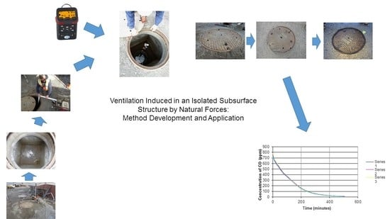
Ventilation Induced in an Isolated Subsurface Structure by Natural Forces: Method Development and Application


1
NorthWest Occupational Health & Safety, North Vancouver, British Columbia V7K1P3, Canada
2
Programa de Pós-Graduação, Universidade Federal Fluminense, Niterói 24210-240, Brazil
3
Escola Politécnica, Universidade Federal do Rio de Janeiro, Rio de Janeiro 21941-972, Brazil
*
Author to whom correspondence should be addressed.
Infrastructures 2019, 4(4), 68; https://0-doi-org.brum.beds.ac.uk/10.3390/infrastructures4040068
Submission received: 28 August 2019
/
Revised: 20 October 2019
/
Accepted: 25 October 2019
/
Published: 31 October 2019
Abstract
:It is believed that isolated subsurface structures of an infrastructure do not ventilate through opening(s) in manhole covers. The literature has almost no information on this topic. This study reports on considerations involved in the development and utilization of a method to study this question. Carbon monoxide (CO) is readily obtainable in engine exhaust, easily detectable at very low concentration, and is relatively safe to handle, which makes it ideal for use as a tracer gas. Transfer into the airspace of the structure was carried out using metal tubing. This study examined the engine operating time and the number of openings in a manhole cover. CO was measured using four instruments in the vertical profile. It was found to generally decrease in a narrow band, initially linearly through a curvilinear region and a linear tail. Clearance of most of the contaminant occurred rapidly during the first part of the process. A decrease to 25 ppm required from 439 min (7 openings) to 1118 min (1 opening). Ambient temperature and near-surface air flow likely influenced these values. The measurement profiles strongly suggest that the atmosphere in the airspace was rapidly and thoroughly well-mixed. The methodology developed and reported here is suitable for a more expanded investigation, the intent being to identify modifications of the design to optimize the process.
1. Introduction
Over the years, some types of workspace have been come to be known as ‘confined spaces.’ Confined spaces are places in which people do not normally work [1]. They may be inaccessible under normal conditions of operation or inactivity. When entry becomes necessary, sometimes special preparation is necessary to gain access. Structures in the subsurface infrastructure that are large enough for entry and performance of work, need to meet the requirements for classification as confined spaces. Structures in the subsurface infrastructure are divisible into two main groups, namely those that are networked together and those that are isolated. Networked structures include manholes and storm chambers, sanitary wastewater collection system, and underground electrical and communication vaults. In both cases, the structures are linked by piping, duct, or some other form of tube. The atmosphere can migrate between structures in the air space of the connecting piping, duct, or tube. Isolated structures, while potentially connected to other structures, do not share a common airspace.
A common characteristic of confined spaces is the boundary surface [2]. Hazardous atmospheres confined by boundary surfaces have resulted in many fatal accidents [2,3,4,5,6,7,8]. The boundary surfaces of subsurface structures in the infrastructure are typically made of concrete and steel. The only defined pathways for air exchange in the subsurface structures containing impervious boundary surfaces are the opening(s) in manhole covers and the access hatches or the open manhole itself.
The technical literature contains considerable conjecture but little substantive information about the confining capabilities of boundary surfaces and the capacity for air exchange, where defined pathways exist. To illustrate, informal inquiry of individuals and groups about the possibility of exchange (ventilation) between the atmosphere in the airspace of a subsurface structure and external atmosphere induced by natural forces, elicits the universal opinion that ventilation does not occur. This opinion is held regardless of the level of education or training or type of work. That is, people educated in occupational health and safety and in confined spaces in particular hold the same view as others.
Ventilation capability of confined spaces in the subsurface infrastructure is an important issue because the safety of passersby and workers who enter and work in these structures depends on the occurrence of continuous air exchange as a means to minimize the concentration of contaminants that have entered. Despite the critical importance of this subject, limited information on this topic exists in the technical literature, as indicated in a recent review [9]. Investigators at the Bureau of Mines studied this question in the mid-1930s and showed that despite common opinion to the contrary, continuous ventilation does occur in the airspace of isolated subsurface manholes, through the opening(s) in the manhole cover [10,11,12,13]. These documents reported on the effect of the number of opening(s) in the manhole cover and the opening area [10], the size and geometry of the structure [11], influence of surface wind on air exchange [12], and the effect of alternate paths of entry [13]. Wiegand and Dunne [14] examined purging through the opened manhole cover through natural influences, including surface air flow.
Lack of information in the published literature opens up the question on how to study ventilation in these structures. Investigators at the Bureau of Mines created concentrated, uniformly distributed, equilibrium mixtures of natural gas or carbon dioxide in the airspace of the structure [10]. The mathematics involved in the study (a constant generation rate during the period of measurement) necessitated careful attention to create and maintain a uniform, immediately-mixed distribution in the airspace. Wiegand and Dunne [14] prepared a finite dilute mixture of N2O by piping compressed gas into the vault from a cylinder and mixed this using a fan (generation rate = 0 during the period of measurement).
Garrison and coworkers [15,16,17,18] examined the mechanical ventilation using a fan in a small model of confined spaces containing various gas mixtures. These studies highlighted the problem of using substances that are normally foreign to these environments and the difficulty in producing the dilute, rapidly, well-mixed atmosphere, required to satisfy the mathematics for uniform dilution during ventilation processes. Recently, McManus [19] and McManus and Haddad [20] explored air exchange between the open atmosphere and the airspace of an isolated subsurface structure through opening(s) in the manhole cover using the more advanced techniques available at this point of time. The method involved a brief introduction of contaminants that are readily encountered in the work environment and air monitoring over time to determine the reduction in concentration induced by the natural ventilation process of the airspace (generation rate = 0 during the period of measurement).
Taken together, the information and comments provided in the articles mentioned above [1,2,3,4,5,6,7,8,10,14] indicated that the desirable characteristics of the contaminant to be used in a study of ventilation induced by natural forces include:
- a normally occurring, easily obtainable substance;
- detectability over a wide range of concentration extending down to zero;
- repeatable preparation of the starting mixture using readily available equipment;
- relative safety in handling and no risk of fire or explosion; and
- passive participation in ventilation processes induced by natural forces.
This study describes considerations involved in undertaking this challenge in a manner that produces a high confidence in the results and provides a stable platform for further study. Demands for establishing and maintaining control over the environment in which the study c occur, introduces further complications that are not often considered or discussed in technical articles. Establishing defensible and repeatable actions that can be taken during the development and implementation of a method in a manner that also creates and provides a safe and healthful environment, within the context of regulatory requirements, is a complex undertaking that is not necessarily apparent when only considering superficial factors.
One of the most important considerations identified in the list, although not directly stated in previous discussions, is health and safety. Discussion about health and safety issues intrinsic in the method and precautionary measures taken to resolve them during research investigations, typically remain undiscussed in technical reports. To illustrate, investigators at the Bureau of Mines utilized mixtures containing natural gas at concentrations necessitated by the detection technology available in the 1930s [10,11,12,13]. These levels posed a fire and explosion hazard. In the work of Wiegand and Dunne [14], the level of N2O in the atmosphere initially expelled from the open manhole during purging induced by natural forces (300 ppm) exceeded the regulatory exposure limit of 50 ppm (parts per million by volume) by a factor of 6.
Recent serious and fatal accidents have focused attention of regulators onto this subject. Workplace regulatory statutes, at minimum, require cover instructors and managers at these facilities who can cover students performing research and investigatory activity. In recognition of the vulnerability to workplace hazards through a lack of education, training, and knowledge, WorkSafeBC—the workplace regulator in the Canadian province of British Columbia—extends coverage to students engaged in unpaid practicums [21]. This policy extends the responsibility to the institution, through instructors and managers, to provide a safe place of work for students engaged in investigative and research activities. This situation imposes an immense challenge onto institutions, managers, and supervisors, to establish and implement a safe system of work when the work to be performed can involve unknown and previously unrecognized hazards. Regulators typically address this burden through a requirement for utilizing a qualified person, an individual possessing education, training, and experience about the hazards and risks involved in performing the activity and strategies for eliminating or, at least, controlling them.
The first decision taken in this situation was to choose a normally occurring, easily obtainable contaminant that is likely to be present in the subsurface isolated structure under study. Decades ago, investigators at the Bureau of Mines have identified automotive fuel vapor, gases of soil origin (such as methane and hydrogen), industrial and domestic fuel gases (such as methane, ethane and acetylene), and CO and CO2 associated with the engine exhaust in these structures [22,23]. More recent study has confirmed the presence of these substances [24].
The literature on fatal accidents strongly suggest that the hazardous atmospheres contained molecules in air [2]. Put another way, most regulatory exposure limits for airborne substances are less than 100 ppm (100 molecules of contaminant per million molecules of air) [25]. The density of this type of contaminated atmosphere is almost indistinguishable from that of the normal atmosphere.
Regulatory exposure limits for gases measured by readily available instruments are 25 ppm (parts per million by volume) for CO; 5000 ppm for CO2; and 25 ppm for NO; 0.2 ppm for NO2, averaged over 8 h. Of further importance are the value concentrations of Immediately Dangerous to Life and Health (IDLH) published by the US National Institute for Occupational Safety and Health (NIOSH) [26]. Respective IDLH values are 1200 ppm for CO; 40,000 ppm for CO2; 100 ppm for NO; and 13 ppm for NO2, averaged over a period of 30 min.
Small gasoline engines emit CO and CO2, some NO and NO2, some water vapor, and some particulates and vapor from unburnt fuel [27]. Absence of reactivity in the natural environment and loss within the period of measurement are important determinants in the choice of contaminant to study. That is, the contaminant must remain stable during the period of measurement in order to ensure that any change in concentration occurs only due to ventilation induced by natural forces and not because of conversion to another substance. Conversion of NO to NO2 can potentially occur through reaction with oxygen and organic substances that might be present in the exhaust [27]. Hence, neither NO nor NO2 is suitable for long duration sampling. Oxidation of CO to CO2 occurs in the atmosphere in the presence of light energy, over an apparent lifespan of several months [28]. This indicates that CO contained in an isolated subsurface structure lacking sunlight would survive, at least, several days and would be suitable for measurement.
CO2 is produced by many sources, such as respiration in roots of plants and respiration by aerobic microorganisms in landfilled materials, as reflected in soil gas [8,19,20,29]. Additional sources of CO2 in the normal environment include exhaust gases from engines. The airspace contains the ambient level of CO2 present in the external atmosphere. Hence, CO2 is not a potential candidate for measurement in the isolated subsurface structures used in this work.
Unburned fuel vapor contains many types of hydrocarbons [27]. Change in composition of gasoline between winter and summer, and differences in emission between operation in cool and cold weather versus warm and hot weather further eliminate the measurement of airborne hydrocarbons from consideration.
The potential for cross-contamination by substances capable of entering the structure from the surrounding air through opening(s) in the manhole cover and from the soil is another consideration. Elimination of the former problem requires isolation of the work area from sources on the contaminant in ambient air. Airspaces that are isolated from the environment normally provide no path for inflow of contamination, except for the openings in the manhole cover. The structure in which this work is proposed comprised a precast concrete base and sides, a concrete top, a steel casting containing a removable manhole cover, and concrete spacer rings that raise the casting to grade level. A thick bead of a mastic caulk inserted between these components prevented migration of water and minimized migration of gas and vapor from the surrounding soil. The concrete base contained no cracks or openings. These requirements also meant that the atmosphere outside the space did not contain the contaminant of interest and that no entry was possible during the test. Hence, the only source of contamination to be measured was that introduced at the start of the test.
Consumption and consequent loss of the substance from the airspace caused by the process of measurement must not unduly influence the output of the instrument. That is, removal of an appreciable quantity of the substance during measurement in a system containing a finite quantity would create an artefact of removal. Given sufficient removal during measurement, this loss could bias the overall measurement. The quantity removed during detection must be negligible compared to the quantity in the airspace. Carbon monoxide sensors, for example, operate through chemical reaction [30]. As a result, molecules of CO are consumed in the process.
The process of measurement must not bias the mechanism of dispersion and self-ventilation through interference with natural forces. Flow induced in the airspace by a source of heat associated with the operation of a sensor or operation of a pump, which removes contaminated air from the instrument for sampling, could induce a motion that would not occur under conditions where the test equipment did not operate. In this regard, an instrument with a passive inflow into sensors seems more appropriate to this investigation than an instrument that actively samples the atmosphere through an internal or external pump. The internal pump in some instruments operates at 1 L/min [30].
The last key concern relates to compatibility of instruments with the environment that they will encounter. Instruments used in confined spaces undergo testing to confirm performance in an ignitable atmosphere. Combustion normally reduces the concentration of organic molecules in the fuel vapor from within the ignitable range to a non-ignitable level in the exhaust.
2. Materials and Methods
This work was performed on the property of a construction contractor located in Burnaby, British Columbia, Canada, a suburb of Vancouver. This company installs and services precast concrete vaults used in underground electrical and communications utilities. The property is located atop a ridge of land and receives little wind. Crews leave the property early in the morning and return late in the afternoon. Otherwise, there is little disturbance of the study location during the day.
The vault offered for this work was previously installed in the ground, following the normal protocol, using customer-specified backfill, spacers to raise the casting to ground level, and a manhole cover with 7 openings—six in the circumference and one in the center. Sections of precast concrete were sealed against leakage using a mastic caulk. The vault had a height of 1.5 m and a volume of 2.5 m3. The vault was not connected to other structures.
Instruments used during these tests included four G460 Multi Gas Detectors (GfG Instrumentation, Inc., Ann Arbor, MI, USA). All instruments contained oxygen, ignitability, and CO and H2S sensors. Two instruments contained CO2 sensors and two contained Photoionization Device (PID) sensors. The instruments were calibrated according to the recommendations of the manufacturer. Dataloggers in the instruments were set to report every minute. The manufacturer indicated that the CO sensor had a resolution of 1 ppm and a tolerance band of ±5 ppm [31]. Other sensors were deactivated following initial testing to confirm the safety of the procedure in order to conserve battery life; entry into the space did not occur.
The instruments were positioned on a photographic light stand (Canadian Studio, Richmond, BC, Canada) (Figure 1) at 38 cm (15 in); 76 cm (30 in); 114 cm (45 in); and 152 cm (60 in) from the ground, respectively. The instruments were activated just prior to insertion into the structure at the beginning of the testing period.
A gasoline-powered Honda engine (GX120, Honda Engines Group, Alpharetta, GA, USA) was used as the source of the exhaust gas to contaminate the air in the vault during testing. The engine was started at an ambient outdoor temperature, using the full-choke setting. The choke was returned to normal position immediately on start-up. At all times, the engine was operated for the minimum amount of time in order to minimize operator exposure to engine exhaust.
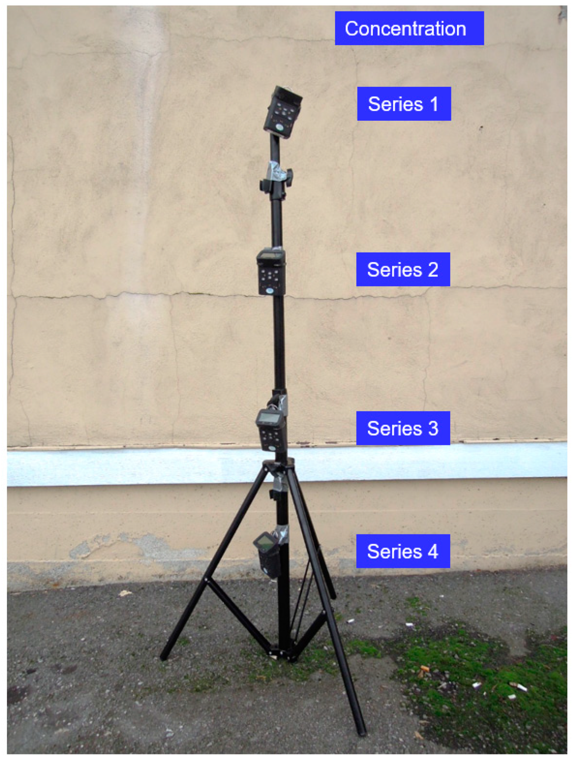
The space was prepared for the daily test in the following manner. The manhole cover was opened the minimum amount needed to accommodate the supply tube (an aluminum tube (75 mm in diameter) containing a 90° elbow.) The engine was started and operated outside the vault and the exhaust was transferred into the bottom. The tube was held against the exhaust port of the engine to ensure an effective seal (Figure 2). During the tests, the engine was operated initially for 180 s, then 60 s, and finally for 30 s. The latter was the minimum time in which to obtain reasonable reproducibility while positioning the tube on the side of the engine and inside the vault. At the end of the period of injection of the exhaust, the manhole cover was then replaced and the atmosphere was allowed to stabilize for 15 min. Just prior to the end of the period of stabilization, the instruments were started up. At the start time, the manhole cover was opened partly and the stand containing the instruments was immediately lowered into the center of the vault and the manhole cover was immediately closed again (Figure 3).
All openings in the manhole cover remained open during the initial series of tests. Subsequently, openings opposite each other in the circumference were plugged two at a time using the mastic caulk described previously. A maximum of six openings in the circumference were closed in this manner, only leaving open the opening in the center. In other series of tests, the opening in the center and one in the circumference were open and in the last series, two positions in the circumference opposite each other were open.
IHSTAT (Industrial Hygiene Statistics) developed and published by the American Industrial Hygiene Association (AIHA) [32] was used for statistical analysis of values within the groups of tests. IHSTAT is an Excel application that determines whether samples are normally or log-normally distributed, in compliance with regulatory standards and guidance values, through goodness of fit tests. AIHA [33] recommends the use of the lognormal distribution for data that appear to be lognormally distributed and for data that are better represented statistically as lognormally distributed or represented by both the normal and lognormal distributions.
The data were subjected to additional statistical analysis to investigate inter-group relationships, using SOFA (Statistics Open For All), Version 1.4.6, an open-source program containing various analytical capabilities [34].
3. Results
Initial testing utilized all available sensors on the instruments in order to confirm safety during the work. Oxygen level in the airspace determined continuously during the tests remained at the normal background level of 20.9%, in almost all situations. On rare occasions, especially during the initial tests in January 2015, oxygen level decreased from 20.9% to 20.7% for very brief periods, during some tests. On other occasions, this decrease persisted for long periods during the day. The cause of these episodes remained undetermined but appeared to be completely unrelated to the tests performed during this work.
The level of CO2 (background + engine exhaust) ranged from 900 ppm to 2400 ppm during early tests. The latter level was less than 50% of the regulatory exposure limit of 5000 ppm, averaged over an 8-h work shift [25]. (The regulatory exposure limit in British Columbia is the threshold limit value published by the American Conference of Governmental Industrial Hygienists.) Subsequent levels ranged from 300 ppm to 400 ppm. These were consistent with the background levels [35]. The CO2 sensors were deactivated to conserve battery energy in order to focus on the measurement of CO.
Hydrocarbon vapors from the unburned fuel were monitored for almost half of the tests. The concentration of hydrocarbon vapors was expressed relative to the concentration of isobutylene (in ppm) used to calibrate the sensor. The concentration of isobutylene was highest during initial measurements in the second half of January (as high as 118 ppm) and decreased steadily to the range of 5 ppm to 7 ppm, as the ambient temperature increased. These concentrations confirmed that gasoline engines emit less unburned fuel vapor in the warmer months of the year. Converting the measured values to concentration of gasoline vapor in air requires multiplication by a conversion factor (1.1) [36] and comparison against the regulatory exposure limit of 300 ppm [25]. Multiplying 118 ppm × 1.1 = 130 ppm. The latter value is considerably less than the regulatory exposure limit. The levels of unburned gasoline vapor measured during these tests were below the threshold of concern. As a result, the PID sensors were deactivated so as to conserve battery energy.
H2S and ignitable substances were undetectable. These sensors were deactivated to conserve battery energy.
Carbon monoxide (CO) became the focus of the study for reasons discussed in the Introduction. The maximum quantifiable concentration was 794 ppm. This was obtainable following a brief operation of the engine (30 s) and provided an ideal means to study ventilation induced by natural forces over a prolonged period of time. In some circumstances, the initial concentration of CO exceeded this value and was not quantifiable. The initial concentration of 794 ppm was many-fold greater than the regulatory exposure limit of 25 ppm averaged over an 8-h work shift [25].
The quality of the exhaust at the beginning of the sample period reflected the ambient temperature at the time of start-up of the engine. The engine remained outdoors and started without any incident on the first pull of the cord, except when the temperature decreased below freezing. The engine produced less CO in summer than in winter for the same conditions of operation. Decrease in concentration of CO in the structure occurred over time when the manhole cover contained one or more openings. The concentration of contaminants in dilute mixtures generally behaved in a predictable manner and decreased to zero, following sufficient time (Figure 4).
Readings from individual instruments generally coalesced to create a single line. The concentrations measured by individual instruments rapidly became indistinguishable from each other. That is, concentrations provided by individual instruments rapidly became almost identical at every level in the vertical profile of the airspace, at every moment, during the period of measurement. Put another way, the concentration measured by individual instruments in the vertical profile was the same for any moment of time. This behavior indicated a process involving thorough and rapid mixing at all levels in the structure.
McManus [19] and McManus and Haddad [20] discussed these and other aspects of the process in considerably more detail. Discussions in this article are focused on the concepts not mentioned in McManus and Haddad [20].
As observable visually, the band of curves generally decreased rapidly in concentration followed by a distinguishable region of intermediate decrease, followed by a region of very slow decrease. This meant that most gaseous contaminant disappeared rapidly from the airspace of the structure. The initial region of rapid decrease was often linear although curvilinearity occurred in some tests. The initial region and the middle region generally required similar time. A point of inflection discernible to the eye generally separated the linear initial region from the curvilinear middle region. On occasion, the curvilinear middle region exhibited an inverted curve that could be described as a hump. The region of slow decrease in concentration (linear tail region) was generally linear and required an extensive period of time.
On occasion, concentration was measured by the instrument in #1 position (top instrument on the stand), sometimes by the instrument in #2 position, and at times #3 position also did not lie within the band of concentration and showed considerable jaggedness. The readings decreased curvilinearly but with a different slope. Despite the displacement of one or more of the curves, the curvilinear decrease remained almost the same in the unaffected curve(s). In other cases, abrupt rapid initial decrease in some concentrations also occurred.
The CO readings provided the basis for calculating the ventilation rate for the system under examination. Table 1 summarizes the results from the characterization of the regions with their measured values (linear initial region and linear tail region), as discussed above. The curves on which Table 1 are based are presented in units of concentration (parts per million) versus time (minutes); (data used to calculate these values are available on request.) Table 1 consolidates the composite curves created from three or four individual curves obtained during each test. From these, values were selected for calculating the slope of the linear initial region, and the linear tail region. The values used to determine the slope of the initial linear region did not include those present in abrupt and abnormal decreases in concentration as seen in some individual curves that were observed during some tests.
The slope expressed in ppm/min/(initial concentration) had units of 1/min since the initial concentration had units of ppm. Hence, this unit multiplied by the volume of the space (2.5 m3) provided an estimate of the rate of ventilation (m3/min) induced by natural forces in that region of the data. Generally, the rate decreased in the two regions (linear initial region and linear tail region). The data showed a general trend of decrease in ventilation rate with a decrease in the number of openings. Temperature and near-surface air motion [19,37], with respect to the time of the year, complicated the clarity in the decrease in ventilation rate that is observable in Table 1. The influence of these factors on the ventilation of isolated subsurface structures during the year remains to be determined.
IHSTAT indicated that, generally, the log-normal distribution better described the data in the groups in the three regions [32]. This was consistent with other analysis of environmental and industrial hygiene data [33,38]. In addition, a high proportion of the geometric standard deviations (GSD) were less than 2.0. This indicated a tight distribution of the data in each group. The GSDs for the groups containing a relative decrease in concentration (ppm/min/(initial concentration), which adjusted for the differences in initial concentration within the group, were generally equal to or smaller than those within the same group, for slopes based on a decrease in absolute concentration (ppm/min). The transformation to the relative decrease in concentration with time, adjusted for the situations where the initial concentration in individual contributors were considerably different.
Rate and effectiveness (efficiency) of ventilation are concepts of major importance in this study. Rate of ventilation depends on the volume of the airspace (2.5 m3 or 90 ft3 as mentioned). Effectiveness (efficiency) of ventilation depends on the previous information plus the area of the opening(s) in the manhole cover. The diameter of the center opening in the manhole cover was 28 mm and the diameter of the outer openings were 29 mm. Previous analysis suggested that the rate of ventilation induced by natural forces was influenced by the number of openings and the position of openings in the manhole cover [10,19,20]. Table 2 summarizes the calculations to determine the numerical value of the rate and the effectiveness of ventilation induced by natural forces.
The results for ventilation rate paralleled the data provided in Table 1, since these results were derived by a multiplication of a constant value (volume of the space). Ventilation effectiveness (efficiency) depended on the area of the opening(s) which changed from group to group in Table 2. Ventilation effectiveness (efficiency) was greatest when the manhole cover contained one or two openings and decreased when more than two openings were present. This finding paralleled data extractable from results published by investigators at the Bureau of Mines but were not highlighted in their reports [9,10,19,20].
The slope of the curves in the curvilinear middle region could not be calculated in the manner used in Table 1 for the linear initial region and the linear tail region because of the necessity to obtain the equations for the curves. The slope at the beginning of the curvilinear middle region was the slope of the linear initial region. Similarly, the slope at the end of the curvilinear middle region was the slope of the linear tail region. The slope in the curvilinear middle region varied with time.
An important consideration in the curvilinear middle region was the mathematical representation of the curves. The curves were fitted to the data points using the curve-fitting function in Microsoft Excel (Table 3). Exponential or second- to fourth-order polynomial curves best fit the data points. Both types of equation provided values of R2 and the correlation coefficient, which was close to the maximum value of 1.0. In some cases, the two types of equations provided almost the same value of R2.
A determination of considerable interest and importance in this investigation was the time required to reach an end-point (Table 4). End-points of interest in occupational health and safety include the regulatory exposure limit (25 ppm averaged over 8-h); action level (half of the regulatory exposure limit) of 12 or 13 ppm at which employers are required to monitor exposures and to take action through various type of controls, to prevent exceedance of the regulatory exposure limit; and the zero level, the true end-point of the study (0 ppm).
Starting concentrations selected for inclusion in Table 4 were similar in magnitude. This means that at least one member in each group was close to or at the maximum starting concentration for CO of 794 ppm. This means that the time to reach the various end-points depended on the number (area) of openings and possibly, as mentioned previously, near-surface air movement and temperature. Clearance to the regulatory exposure limit of 25 ppm ranged from 439 min to 1203 min. Clearance to the action level of 12 ppm could require more than 1000 min for a small numbers of openings. Clearance to the zero level could require 24 h (1440 min) or more for a small numbers of openings in the manhole cover.
4. Discussion
This article introduces and discusses considerations involved in the study of ventilation of an isolated subsurface structure induced by natural forces. These include selection of a commonly occurring, readily obtainable air contaminant that is detectable at very low concentrations, which is easily prepared in a uniform starting concentration using readily available equipment and which imposes no overexposure or fire or explosion hazard when handled appropriately with due care. These considerations while superficially simple could require considerable in-depth investigation to confirm the suitability of a particular course of action. These considerations are seldom discussed in the literature. Faulty decision-making could lead and has led to injury and death.
Carbon monoxide is a readily available air contaminant produced by gasoline engines. It is easily manipulated to generate a hazardous atmosphere for study, as demonstrated in the Method. Molecules of CO have molecular weight of 28 units, one unit different from the molecular weight of the average molecule in air (29 units, mostly nitrogen and oxygen). Hence, an atmosphere containing CO as a contaminant is physically indistinguishable from an atmosphere lacking these molecules. The only way to identify and quantify the presence of CO is a chemical reaction inside the CO sensor contained in the detecting instrument. CO is chemically stable in air for a long period [28] and, therefore, is suitable for detecting change in concentration due to the effect of ventilation. These characteristics are highly advantageous for study as there is no concern about a substance that is foreign to the industrial environment. In addition, CO introduced into the chamber for study is easily isolated from CO produced by other sources in the environment.
The outdoor environment is uncontrollable. It fluctuates according to daily and annual cycles [19,20,37]. Hence, conditions of measurement are not controllable to the extent desired by investigators seeking to vary only one parameter per test. This reality confronted investigators at the Bureau of Mines, as reflected in the comments made in their reports [10,11,12,13], as well as in this situation. The reply to this criticism was that the outdoor environment contains phenomena yet to be discovered and characterized, and was only briefly mentioned in this report (abrupt initial decrease in concentration) and in other reports, by the authors of this document [19,20]. These phenomena could completely defy presumptions [19,20,37]. Only following thorough investigation and characterization could one attempt to duplicate and control the outdoor conditions in the laboratory.
The quest described in these reports [19,20] encountered considerable difficulty for several explicable and sometimes inexplicable reasons. Despite preparation of the atmospheric mixtures from test to test in a consistent and repeatable manner as possible, the starting concentrations within an identical group of replicates, were often considerably different. Comparison against the initial concentration compensated for the abrupt initial losses and other unobserved irregularities. The normal expectation is to presume an influence of ambient temperature, as the engines are known to produce less CO when started warm or hot. However, in this case the temperature of the engine at start-up was always the ambient temperature at the end of the night and not the operating temperature of the engine.
An additional complicating factor was battery failure in the monitoring instruments. In these cases, the batteries failed before the concentration decreased sufficiently to reach one or more of the chosen benchmarks used in Table 4. Decrease of concentration to a low level required extreme performance from the batteries used in these instruments and deactivation of all but the CO sensor.
Given the preceding limitations and difficulties and the importance of the estimate, the decision was taken in preparing Table 4 to select a test from each group of replicates that contained the highest possible concentration. The duration for that test most closely reflected the influence of the number of opening(s) in the manhole cover, ambient temperature, and the near-surface airflow. Collectively, these tests provided some basis to investigate the question about how long it takes for the concentration to decrease to at least the regulatory exposure limit. The data provided in Table 4 were selected independent of each other. For an engine operating time of 30 s, values for clearance time most closely showed the influence of the opening area on the ventilation rate, as reported by the investigators at the Bureau of Mines [10].
One of the concerns mentioned in the Introduction that was unresolved in previous discussion, was consumption of the substance under investigation through the process of measurement. Inspection of the output from the instruments indicated that very low levels of CO (1 or 2 ppm) remained constant for a considerable period of time. This is a preliminary indicator that consumption of CO molecules during detection by the CO sensor did not materially affect the output of the instrument at very low levels.
Oxidation of CO in the CO electrochemical sensor occurred in the following manner [30]:
CO + H2O → CO2 + 2H+ + 2e−
This situation indicated that detection of each molecule of CO created a current of 2 electrons. Completion of the circuit involved reduction of O2 and consumption of the 2 electrons. The CO sensor requires 50 nA/ppm of CO to be detected [39]; (nA is nanoAmpere, a unit of current flow). The number of molecules of CO converted at the level of 1 ppm was (50 nA/ppm of CO/instrument) × (10−9 Coulombs/sec/nA) × (6.2415 × 10¹⁸ electrons/Coulomb) × (molecule of CO consumed/2 electrons) × (4 instruments) = 6.24 × 10¹¹ molecules of CO molecules consumed/sec/ppm of CO detected by all 4 instruments.
Instrumental and atmospheric observations during this study indicated that the airspace was constantly in motion and rapidly and thoroughly well-mixed [19,20]. This meant that the entire volume of air (2.5 m3) and the molecules of CO that it contained were potentially in contact with the CO sensors in the instruments. The number of molecules of CO in the airspace at a concentration of 1 ppm would be 2.5 m3 × 1000 L/m3 × (1 molecule of CO/1,000,000 molecules of air) × (mole/24.45 L) × (6.023 × 10²³ molecules of air/mole) = 6.16 × 10¹⁹ molecules of CO. This differential suggested that at the rate of consumption calculated above, the instrument would read 1 ppm for a considerable period of time.
5. Conclusions
This work investigated and demonstrated the creation and operation of an effective, safe, and stable system for the study of ventilation induced by natural forces in an isolated subsurface structure, a type of confined space. Devising a methodology for the study of behavior of this confined atmosphere necessitates consideration about health and safety, and identification of a substance that is readily available and easily manipulated to create a contaminated atmosphere in a reproducible and controllable manner. Satisfying these requirements requires considerable deliberation, prior to the start of testing. CO is the obvious choice for study as a contaminant. It is easily detected at very low concentration and because its molecular weight is almost identical to other molecules in normal air, it does not actively influence the ventilation processes. Exhaust from a gasoline engine is a suitable source of CO for this type of study. Decrease in concentration of CO is divisible into a linear initial region, a curvilinear middle region, and a linear tail region. The ventilation rate (under as closely replicable conditions as possible) for a system where generation rate = 0 was found to decrease with increasing number of openings (opening area) in the manhole cover. Ventilation effectiveness (efficiency) was greatest for one or two openings. Ventilation rate in the replicates was best described by the lognormal distribution. The methodology developed and reported here is suitable for more expanded investigation, the outcome being the identification of design modifications for an optimization of the process.
Author Contributions
The following aspects of this article received respective contributions: Conceptualization, T.N.M.; methodology, T.N.M.; investigation, T.N.M.; resources, A.H.; writing—original draft preparation, T.N.M.; writing—review and editing, T.N.M. and A.H.; supervision, A.H.; project administration, A.H.; funding acquisition, A.H.
Funding
This research received no external funding.
Acknowledgments
Thomas Neil McManus received a scholarship from CAPES (Coordenação de Aperfeiçoamento de Pessoal de Nível Superior), Brasilia, DF, Brasil. Assed Haddad received a grant from CNPq (Conselho Nacional de Desenvolvimento Científico e Tecnológico), formerly Conselho Nacional de Pesquisas, Brasilia, DF, Brasil (the Brazililian National Research Council) in pursuit of this work. Special thanks are due to Jack Eusebio of Fred Thompson Contractors, Burnaby, British Columbia, Canada for permission to work on their premises during this work and to Bob Henderson of GfG Instrumentation Inc. for providing the instruments used during this work.
Conflicts of Interest
The authors declare no conflict of interest.
References
- McManus, T.N.; Green, G. The Confined Space Training Program, Worker Handbook; Training by Design, Inc.: North Vancouver, BC, Canada, 2004. [Google Scholar]
- McManus, T.N. Safety and Health in Confined Spaces; CRC Press/Lewis Publishers: Boca Raton, FL, USA, 1998. [Google Scholar]
- NIOSH (National Institute for Occupational Safety and Health). Worker Deaths in Confined Spaces; (DHHS/PHS/CDC/NIOSH Pub. No. 94-103); Department of Health and Human Services, Public Health Service, Center for Disease Control, National Institute for Occupational Safety and Health: Cincinnati, OH, USA, 1994. [Google Scholar]
- NIOSH (National Institute for Occupational Safety and Health). Carbon Monoxide Poisoning and Death After the Use of Explosives in a Sewer Construction Project; DHHS (NIOSH) Publication No. 98-122; Department of Health and Human Services, National Institute for Occupational Health: Cincinnati, OH, USA, 1998. [Google Scholar]
- OSHA (Occupational Safety and Health Administration). Selected Occupational Fatalities Related to Toxic and Asphyxiating Atmospheres in Confined Work Spaces as Found in Reports of OSHA Fatality/Catastrophe Investigations; U.S. Department of Labor, Occupational Safety and Health Administration (U.S. DOL/OSHA): Washington, DC, USA, 1985. [Google Scholar]
- OSHA (Occupational Safety and Health Administration). Fatality and Catastrophe Investigation Summaries; U.S. Department of Labor, Occupational Safety and Health Administration (U.S. DOL/OSHA): Washington, DC, USA, 2018. Available online: www.osha.gov/pls/imis/accidentsearch.html (accessed on 9 December 2018).
- NIOSH (National Institute for Occupational Safety and Health). Fatality Assessment and Control Evaluation (FACE) Program; Department of Health and Human Services, Centers for Disease Control and Prevention, National Institute for Occupational Safety and Health: Cincinnati, OH, USA, 2018. Available online: www.cdc.gov/niosh/face/ (accessed on 9 December 2018).
- Smith, P.A.; Lockhart, B.; Besser, B.W.; Michalskic, M.A.R. Exposure of unsuspecting workers to deadly atmospheres in below-ground confined spaces and investigation of related whole-air sample composition using adsorption gas chromatography. J. Occup. Environ. Hyg. 2014, 11, 800–808. [Google Scholar] [CrossRef] [PubMed]
- McManus, T.N.; Haddad, A.N. Natural Ventilation in Isolated Subsurface Structures in the Infrastructure: A Review. Environ. Nat. Resour. Res. 2019, 2, 61–74. [Google Scholar] [CrossRef]
- Jones, G.W.; Miller, W.E.; Campbell, J.; Yant, W.P. Ventilation of Manholes. 1. Effect of Holes in the Covers on Natural Ventilation (RI 3307); Department of the Interior, Bureau of Mines: Washington, DC, USA, 1936. [Google Scholar]
- Jones, G.W.; Miller, W.E.; Campbell, J.; Yant, W.P. Ventilation of Manholes. 2. Effect of the Size of the Manhole on Natural Ventilation (RI 3343); Department of the Interior, Bureau of Mines: Washington, DC, USA, 1937. [Google Scholar]
- Jones, G.W.; Baker, E.S.; Campbell, J. Ventilation of Manholes. 3. Effect of Wind Velocity on Natural Ventilation (RI 3412); Department of the Interior, Bureau of Mines: Washington, DC, USA, 1938. [Google Scholar]
- Jones, G.W.; Miller, W.E.; Campbell, J. Ventilation of Manholes. 4. Effect of Vertical Ducts in Combination with Openings in Manhole Covers on the Natural Ventilation (RI 3496); Department of the Interior, Bureau of Mines: Washington, DC, USA, 1940. [Google Scholar]
- Wiegand, K.; Dunne, S.P. Radon in the workplace—A study of underground BT structures. Ann. Occup. Hyg. 1996, 40, 569–581. [Google Scholar] [CrossRef]
- Garrison, R.P.; Nabar, R.; Erig, M. Ventilation to eliminate oxygen deficiency in a confined space. Part I: A cubical model. Appl. Indust. Hyg. 1989, 4, 1–11. [Google Scholar] [CrossRef]
- Garrison, R.P.; Erig, M. Ventilation to eliminate oxygen deficiency in a confined space—Part II: Non-cubical models. Appl. Indust. Hyg. 1989, 4, 260–268. [Google Scholar] [CrossRef]
- Garrison, R.P.; Erig, M. Ventilation to eliminate oxygen deficiency in a confined space—Part III: Heavier-than-air characteristics. Appl. Occup. Environ. Hyg. 1991, 6, 131–140. [Google Scholar] [CrossRef]
- Garrison, R.P.; Lee, K.; Park, C. Contaminant reduction by ventilation in a confined space model—toxic concentrations versus oxygen deficiency. Am. Indust. Hyg. Assoc. J. 1991, 52, 542–546. [Google Scholar] [CrossRef] [PubMed]
- McManus, T.N. Natural Ventilation of Isolated Subsurface Structures in the Infrastructure. Master’s Thesis, Universidade Federal Fluminense, Programa de Pós Graduação em Engenharia Civil, Niteroí, Brazil, 2016. [Google Scholar]
- McManus, T.N.; Haddad, A. Ventilation of an isolated subsurface structure induced by natural forces. Infrastructures 2019, 4, 33. [Google Scholar] [CrossRef]
- WorkSafeBC. Did you Know? Unpaid Practicum Students are Eligible for Workers’ Compensation Coverage. Available online: https://www.worksafebc.com/en/resources/health-safety/information-sheets/did-you-know-unpaid-practicum-students-are-eligible-for-workers-compensation-coverage?lang=en (accessed on 11 August 2018).
- Katz, S.H.; Meiter, E.R.; Bloomfield, J.J. Gas Hazards in Street Manholes (RI 2710); Department of the Interior, Bureau of Mines: Washington, DC, USA, 1925. [Google Scholar]
- Jones, G.W.; Perrott, G.S.J. Gases in Manholes: A Survey of a Utility in Boston, Mass (RI 3109); Department of the Interior, Bureau of Mines: Washington, DC, USA, 1931. [Google Scholar]
- IEEE (Institute of Electrical and Electronic Engineers). Preventing and Mitigating Manhole Events. In White Paper Prepared by IEEE Insulating Conductors Committee—C34D; Institute of Electrical and Electronic Engineers: New York, NY, USA, 2015. [Google Scholar]
- ACGIH (American Conference of Governmental Industrial Hygienists). TLVs and BEIs for Chemical Substances and Physical Agents & Biological Exposure Indices; American Conference of Governmental Industrial Hygienists: Cincinnati, OH, USA, 2017. [Google Scholar]
- NIOSH (National Institute for Occupational Safety and Health). Immediately Dangerous to Life or Health (IDLH) Values; Centers for Disease Control and Prevention, National Institute for Occupational Safety and Health: Cincinnati, OH, USA, 2019. Available online: https://www.cdc.gov/niosh/idlh/default.html (accessed on 18 August 2018).
- Seinfeld, J.H.; Pandis, S.N. Atmospheric Chemistry and Physics—From Air Pollution to Climate Change; Wiley: New York, NY, USA, 1998. [Google Scholar]
- Reeves, C.E.; Penkett, S.A.; Baugitte, S.; Law, K.S.; Evans, M.J.; Bandy, B.J.; Monks, P.S.; Edwards, G.D.; Phillips, G.; Barjat, H.; et al. Potential for photochemical ozone formation in the troposphere over the North Atlantic as derived from aircraft observations during ACSOE. J. Geophys. Res. 2002, 7, 4707. [Google Scholar] [CrossRef]
- Ryan, M.G.; Law, B.E. Interpreting, measuring, and modeling soil respiration. Biogeochem 2005, 73, 3–27. [Google Scholar] [CrossRef]
- Chou, J. Hazardous Gas Monitors: A Practical Guide to Selection, Operation, and Applications; McGraw-Hill Professional: New York, NY, USA, 1999. [Google Scholar]
- GFG (Gesellschaft für Gerätebau) Instrumentation. G460 Multi-Gas Detector; GfG Instrumentation Inc.: Ann Arbor, MI, USA, 2015; Available online: http://www.gfg-inc.com/englisch/produkte/g460.html (accessed on 7 June 2019).
- AIHA (American Industrial Hygiene Association). IHSTAT (Industrial Hygiene Statistics); American Industrial Hygiene Association: Falls Church, VA, USA, 2016; Available online: https://www.aiha.org/get-involved/VolunteerGroups/Pages/Exposure-Assessment-Strategies-Committee.aspx (accessed on 9 December 2018).
- Jahn, S.D.; Bullock, W.H.; Ignacio, J. (Eds.) A Strategy for Assessing and Managing Occupational Exposures, 4th ed.; American Industrial Hygiene Association: Falls Church, VA, USA, 2015. [Google Scholar]
- SOFA (Statistics Open for All). SOFA (ver. 1.4.6); Paton-Simpson & Associates Ltd.: Auckland, NZ, USA, 2015; Available online: http://www.sofastatistics.com/home.php (accessed on 23 December 2018).
- Lide, D.R. Handbook of Chemistry and Physics on CD-ROM; Version 2006; CRC Press; Taylor & Francis Group: Boca Raton, FL, USA, 2006. [Google Scholar]
- GfG (Gesellschaft für Gerätebau) Instrumentation. 2009 Chemical Ionization Potential (eV) and 10.6 eV Correction Factors (CF) (TN2004); GfG Instrumentation: Ann Arbor MI, USA, 2009; Available online: https://goodforgas.com/wp-content/uploads/2013/12/TN2004_PID_gas_table_01_16_09.pdf (accessed on 9 December 2018).
- McManus, T.N.; Haddad, A. Surface air movement: An important contributor to ventilation of isolated subsurface structures? Infrastructures 2019, 4, 23. [Google Scholar] [CrossRef]
- Leidel, N.A.; Busch, K.A.; Lynch, J.R. Occupational Exposure Sampling Manual (DHEW (NIOSH) Publication No. 77-173); Department of Health, Education, and Welfare (US), Public Health Service, Center for Disease Control, National Institute for Occupational Safety and Health: Cincinnati, OH, USA, 1977. [Google Scholar]
- City Technology. Product data sheet, 2CF3 Carbon monoxide CiTiceL®; City Technology Ltd.: Portsmouth, UK, 2017. [Google Scholar]
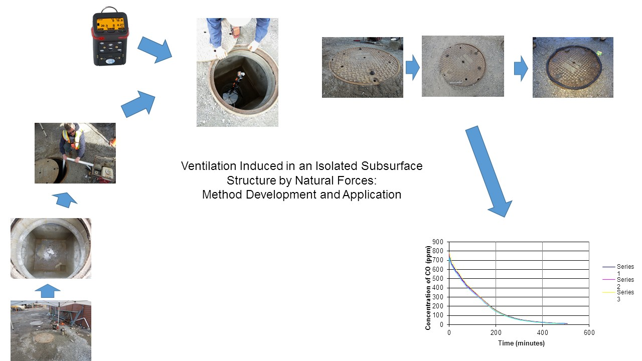
Figure 1.
Instrument stand + instruments. ‘Series’ corresponds to labels used in Figure 4 showing the decrease in concentration of CO with time.
Figure 1.
Instrument stand + instruments. ‘Series’ corresponds to labels used in Figure 4 showing the decrease in concentration of CO with time.

Figure 2.
Transferring exhaust gas into the chamber. The engine was left outdoors at all times and was started ‘cold’ using the choke on the first pull of the starter cord. When the engine started, the choke was immediately disabled and the exhaust gases were transferred into the chamber using the tubing. The tube was held tightly against the engine to prevent the escape of the exhaust gas into the work area. (Note: Heat-resistant gloves were worn during the actual transfer of exhaust gas. The metal of the tubing rapidly became hot to the touch.)

Figure 3.
The instruments in position at the beginning of sample collection just prior to reclosing the manhole cover. The orange color on the displays indicates the alarm condition caused by CO at a concentration of 25 ppm. The instruments entered the alarm condition almost immediately on insertion into the subsurface structure.

Figure 4.
Decrease in concentration of CO in the airspace of the structure with time (16 December 2015). Generally the concentration of CO decreased along a smooth band where the relative position of the readings remained the same. Series 1 to Series 3 reflected the position of the instruments on the stand from top to bottom.


Table 1.
Summary of CO levels measured during this study of ventilation by natural forces in an isolated subsurface structure.
Table 1.
Summary of CO levels measured during this study of ventilation by natural forces in an isolated subsurface structure.
| Characteristics | Slope | |||||
|---|---|---|---|---|---|---|
| Engine Run Time (s) | Number of | Geometric Mean (ppm/min *) | Geometric Standard Deviation | Geometric Mean (ppm/min/(Initial conc) *) | Geometric Standard Deviation | |
| Openings | Tests | |||||
| Linear Initial Region | ||||||
| 180 | 7 | 5 | 4.1 | 1.36 | 0.0048 | 1.27 |
| 60 | 7 | 10 | 4.14 | 1.66 | 0.0072 | 1.39 |
| 30 | 7 | 6 | 4.11 | 1.37 | 0.0056 | 1.22 |
| 30 | 5 (March) | 4 | 4.13 | 1.32 | 0.0055 | 1.29 |
| 30 | 5 (June) | 4 | 4.44 | 1.12 | 0.0070 | 1.15 |
| 30 | 3 | 7 | 1.66 | 2.30 | 0.0049 | 1.28 |
| 30 | 2 (cent + circ) | 11 | 1.59 | 1.42 | 0.0025 | 1.49 |
| 30 | 2 (circ only) | 11 | 1.10 | 2.08 | 0.0041 | 1.28 |
| 30 | 1 | 17 | 0.684 | 1.31 | 0.0017 | 1.32 |
| Linear Tail Region | ||||||
| 180 | 7 | 5 | 0.159 | 3.04 | 0.0048 | 1.27 |
| 60 | 7 | 10 | 0.0974 | 1.46 | 0.0045 | 1.59 |
| 30 | 7 | 6 | 0.104 | 1.39 | 0.0053 | 1.32 |
| 30 | 5 (March) | 4 | 0.042 | 1.13 | 0.0023 | 1.38 |
| 30 | 5 (June) | 4 | 0.0536 | 1.36 | 0.0032 | 1.4 |
| 30 | 3 | 7 | 0.0398 | 1.94 | 0.0017 | 1.26 |
| 3 | 2 (cent + circ) | 11 | 0.0982 | 1.81 | 0.0013 | 1.32 |
| 30 | 2 (circ only) | 11 | 0.0373 | 2.04 | 0.0027 | 1.72 |
| 30 | 1 | 17 | 0.0692 | 2.15 | 0.0015 | 1.83 |
Notes: * Geometric mean in this situation is the antilogarithm of the mean of the logarithms of the measured values expressed in the units stated here. Following are the periods during which these trials occurred: operating time of 180 s—mid-January; operating time of 60 s—late January to mid-February; operating time of 30 s, 7 openings—mid- to late February; operating time of 30 s, 5 openings—early March and early June; operating time of 30 s, 3 openings—late June to mid-July; operating time of 30 s, with 2 circumferential openings opposite each other—mid-July to early August; operating time of 30 s, one central opening—late October to mid-November; operating time of 30 s, two openings, center + circumference—mid-November to late February. (cent + circ) indicates that one opening was in the center and the other on the circumference. (circ only) indicates that the openings were on opposite sides of the circumference. (March) and (June) indicate that this work occurred only during these months.
Table 2.
Summary of rate of ventilation of the airspace by natural forces.
| Characteristics | Relative Rate | Natural Ventilation Rate | Ventilation Effectiveness (Efficiency) | ||||
|---|---|---|---|---|---|---|---|
| Openings | Area | ||||||
| (mm2) | (in2) | (1/min) | (L/min) | (ft3/min) | (mL/min/mm2) | (ft3/min/in2) | |
| Linear Initial Region | |||||||
| 7 (average) | 4579 | 7.10 | 0.0064 | 16.0 | 0.576 | 3.49 | 0.081 |
| 5 (March) | 3528 | 5.47 | 0.0055 | 13.8 | 0.495 | 3.91 | 0.090 |
| 5 June | 3528 | 5.47 | 0.0070 | 17.5 | 0.630 | 4.96 | 0.115 |
| 3 | 1937 | 3.00 | 0.0049 | 12.3 | 0.441 | 6.35 | 0.147 |
| 2 (cent + circ) | 1276 | 1.98 | 0.0026 | 6.5 | 0.234 | 5.09 | 0.118 |
| 2 (circ only) | 1321 | 2.05 | 0.0041 | 10.3 | 0.369 | 7.80 | 0.180 |
| 1 | 616 | 0.95 | 0.0040 | 10 | 0.360 | 16. 2 | 0.379 |
| Linear Tail Region | |||||||
| 7 average | 4579 | 7.10 | 0.0050 | 12.5 | 0.450 | 2.73 | 0.063 |
| 5 March | 3528 | 5.47 | 0.0023 | 5.75 | 0.207 | 1.63 | 0.038 |
| 5 June | 3528 | 5.47 | 0.0032 | 8.00 | 0.288 | 2.27 | 0.053 |
| 3 | 1937 | 3.00 | 0.0016 | 4.00 | 0.144 | 2.07 | 0.048 |
| 2 (cent + circ) | 1276 | 1.98 | 0.0013 | 3.25 | 0.117 | 2.55 | 0.059 |
| 2 (circ only) | 1321 | 2.05 | 0.0027 | 6.75 | 0.243 | 5.11 | 0.119 |
| 1 | 616 | 0.95 | 0.0015 | 3.75 | 0.135 | 6.09 | 0.142 |
Notes: (cent + circ) indicates that one opening was in the center and the other on the circumference. (circ only) indicates that the openings were on the opposite sides of the circumference. Following are the periods during which these trials occurred: operating time of 180 s—mid-January; operating time of 60 s—late January to mid-February; operating time of 30 s, 7 openings—mid- to late February; operating time of 30 s, 5 openings—early March and early June; operating time of 30 s, 3 openings—late June to mid-July; operating time of 30 s, 2 circumferential openings opposite each other—mid-July to early August; operating time of 30 s, one central opening—late October to mid-November; operating time of 30 s, two openings, center + circumference—mid-November to late February. (March) and (June) indicate that this work occurred during these months.
Table 3.
Curve-Fitting using Microsoft Excel of Data Points in the Curvilinear Middle Region.
| Characteristics | Best Equation Fit to the Curve | ||||||
|---|---|---|---|---|---|---|---|
| Engine Run Time | Number of | Exp | Exp/Poly | Exp = Poly Poly = Exp | Poly/Exp | Poly | |
| Sec | Openings | Tests | |||||
| 180 | 7 | 5 | 2 | 3 | |||
| 60 | 7 | 10 | 1 | 6 | 3 | ||
| 30 | 7 | 6 | 6 | ||||
| 30 | 5 (March) | 4 | 1 | 2 | 1 | ||
| 30 | 5 (June) | 4 | 4 | ||||
| 30 | 3 | 7 | 3 | 4 | |||
| 30 | 2 (cent + circ) | 10 | 2 | 2 | 1 | 2 | 3 |
| 30 | 2 (circ only) | 11 | 2 | 4 | 2 | 3 | |
| 30 | 1 | 17 | 1 | 6 | 4 | 6 | |
Notes: Exp means the exponential equation provided the best fit to the curve. Exp/Poly means that the exponential equation provided a slightly better fit to the curve. Exp = Poly and Poly = Exp indicate that both equations provided an equal fit to the curve. Poly/Exp means that the polynomial equation provided a slightly better fit to the curve. Poly means that the polynomial equation provided the best fit to the curve. Exp/Poly and Poly/Exp indicate that the fits to the curve were very close. In all cases, R2 values were very close to 1.0, the maximum value. Following are the periods during which these trials occurred: operating time of 180 s—mid-January; operating time of 60 s—late January to mid-February; operating time of 30 s, 7 openings—mid- to late February; operating time of 30 s, 5 openings—early March and early June; operating time of 30 s, 3 openings—late June to mid-July; operating time of 30 s, 2 circumferential openings opposite each other—mid-July to early August; operating time of 30 s, one central opening—late October to mid-November; operating time of 30 s, two openings, center + circumference—mid-November to late February.
Table 4.
Time Needed for Concentration of CO to Decrease to the Levels of Interest.
| Date | Engine Run Time | Openings in Manhole Cover | Starting Conc. | Time for Concentration to Decrease to | |||
|---|---|---|---|---|---|---|---|
| No. | Area | Exposure Limit (25 ppm) | Action Level (12 ppm) | Zero Level (0 ppm) | |||
| Sec | mm2 | ppm | min | min | Min | ||
| 28.01.2015 | 180 | 7 | 4579 | 772 | 769 | 870 | N Obt |
| 10.02.2015 | 60 | 7 | 4579 | 772 | 534 | 759 | 1021 |
| 24.02.2015 | 30 | 7 | 4579 | 779 | 439 | N Av | N Obt |
| 06.03.2015 | 30 | 5 | 3528 | 777 | 630 | 962 | N Obt |
| 08.06.2015 | 30 | 5 | 3528 | 740 | 663 | 872 | N Obt |
| 03.07.2015 | 30 | 3 | 1937 | 737 | 880 | N Obt | N Obt |
| 24.02.2016 (cent + circ) | 30 | 2 | 1276 | 766 | 1203 | N Obt | N Obt |
| 30.07.2015 (circ only) | 30 | 2 | 1321 | 744 | 990 | N Obt | N Obt |
| 07.12.2015 | 30 | 1 | 616 | 770 | 1118 | N Obt | N Obt |
Notes: No. is number of openings. Conc. is concentration. (cent + circ) indicates that one opening was in the center and the other on the circumference. (circ only) indicates that the openings were on opposite sides of the circumference. N Obt indicates that the value was not obtainable from the data available.
© 2019 by the authors. Licensee MDPI, Basel, Switzerland. This article is an open access article distributed under the terms and conditions of the Creative Commons Attribution (CC BY) license (http://creativecommons.org/licenses/by/4.0/).
Share and Cite
MDPI and ACS Style
McManus, T.N.; Haddad, A. Ventilation Induced in an Isolated Subsurface Structure by Natural Forces: Method Development and Application. Infrastructures 2019, 4, 68. https://0-doi-org.brum.beds.ac.uk/10.3390/infrastructures4040068
AMA Style
McManus TN, Haddad A. Ventilation Induced in an Isolated Subsurface Structure by Natural Forces: Method Development and Application. Infrastructures. 2019; 4(4):68. https://0-doi-org.brum.beds.ac.uk/10.3390/infrastructures4040068
Chicago/Turabian StyleMcManus, Thomas Neil, and Assed Haddad. 2019. "Ventilation Induced in an Isolated Subsurface Structure by Natural Forces: Method Development and Application" Infrastructures 4, no. 4: 68. https://0-doi-org.brum.beds.ac.uk/10.3390/infrastructures4040068