Geometric and Operational Features of Horizontal Curves with Specific Regard to Skidding Proneness

Abstract

(1) Run-off-road (ROR) crashes are a crucial issue worldwide, resulting in a disproportionate number of traffic deaths. In safety research, macro-level analysis on large datasets is usually conducted by linking explanatory variables to ROR crash frequency/severity. Micro-analysis approaches, like the one used in this study, are instead less frequent. (2) A comprehensive Italian Fatal + Injury (FI) crash dataset was filtered to identify two-way two-lane rural road curves on the national road network on which more than one ROR FI crash (i.e., at least two crashes) in the observation period of four years had occurred. The typical features of the ROR FI crashes and the recurrent geometric (characteristics of tangents and curves) and operational features (inferred speeds, acceleration/decelerations) of the crash sites were reconstructed. (3) The main contributory factors in ROR FI crashes are: wet pavements, speeding, and distraction. Sites with a relevant history of ROR FI crashes present recurrent safety issues such as inadequate horizontal curve coordination, an insufficient tangent length for decelerating, and inferred operating speeds comparable/higher than the inferred design speeds. (4) Based on findings, some practical suggestions for road safety management and maintenance are proposed through specific indicators and countermeasures (speed, perception, and friction related).

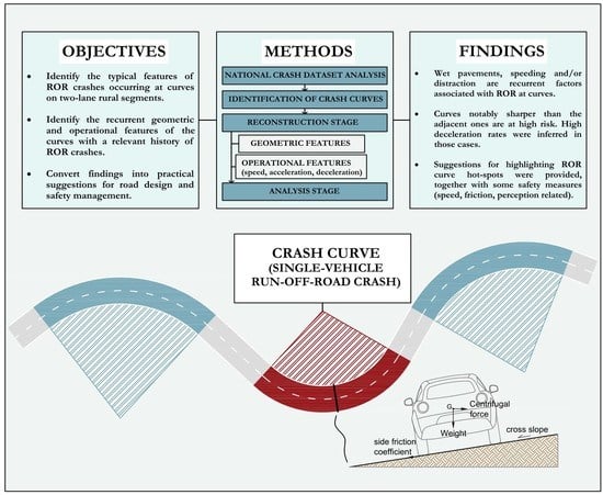
1. Introduction

Among all the crash types, run-off-road (ROR) crashes are a major concern worldwide, given the considerable number of fatalities and serious injuries related to them (see [1,2,3]). These are typically single-vehicle accidents with few interactions with other drivers. In Europe, overall, single vehicle collisions result in about one third of all deaths on roads [4], with most of them occurring in rural environments. The problem is even worse in the United States, particularly for ROR crashes, since fatalities resulting from them account for about half of all traffic fatalities [3].

Clearly, a remarkable number of single-vehicle rural run-off-road crashes (henceforth referred to as ROR crashes) may occur at curves, which involves design aspects that should be highlighted while conducting safety analyses on existing roads [5]. For example, a study by SWOV (Institute for Road Safety Research) [6] (as reported in [4]) highlighted that in a vast majority of ROR crashes at curves (about 90%), the curve radius was inappropriate for the posted speed limit. Moreover, considering detailed statistics from Italy (2014–2017 [7]), ROR crashes at curves with at least one injured person involved accounted for about 3% of all fatal + injury recorded crashes. However, the percentage of fatalities from curve ROR crashes among all fatal crashes is more than double at about 7%. Specifically focusing on undivided two-way rural roads, the disproportion between single-vehicle ROR fatal and fatal + injury crashes increases, about 4% and 1% among the total fatal and fatal + injury crashes, respectively.

Among the main causes of ROR crashes, speed, distraction, and fatigue play an important role (see [4]). Moreover, when specifically focusing on curves, the occurrence of ROR crashes may be influenced, among the other factors, by these road design aspects:

• Geometric curve design, in particular a sharp radius of curvature (see [6,8]);
• Tire-road friction, particularly the side friction available in different conditions [9,10]; and
• Road design consistency, which is intrinsically related to the drivers’ expectations.

In detail, while the first two factors are essentially physically-based and interact between them (design speeds, side friction, and the radii of curvature are typically related), the third factor is more complex. In recent research [11,12], it was shown how crash rates at curves may be influenced by the design characteristics of nearby road elements. For example, drivers, especially if unfamiliar with the road [13], may not expect a sharp curve after a very long tangent. The occurrence of the latter was actually found to be a recurrent safety problem, especially for two-way two-lane rural roads [5].

Research in this field usually includes these above-mentioned factors while investigating ROR crashes. In particular, statistical techniques (e.g., [1,14,15]) are used to capture the most relevant factors that may influence both the occurrence and severity of ROR crashes. However, as previously explained, the most relevant factors may be inter-dependent, both design- and human-related, and may be site-specific. For this reason, in this study, the analysis of ROR crashes was conducted from a “micro” perspective, which has rarely been performed in the literature. In detail, the analysis focused on specific sites with a previous remarkable history of ROR crashes through in depth study of the accident contributory factors and the geometric and operational characteristics of the selected road sites (see [16,17,18]). In this way, specific patterns may be revealed, which are difficult to find with the usual macro-level modeling strategies.

In detail, the study aimed at answering the following research questions:

• What are the typical features of ROR crashes occurring at curves on rural roads, in particular two-way two-lane rural segments?
• What are the recurrent road geometric and operational characteristics of segments including the highlighted curves with a relevant history of ROR crashes?
• Which of the previously highlighted aspects can be useful, and in which way, from a road safety management perspective?

To answer these research questions, two-way two-lane rural road sites seriously affected by ROR crashes at curves belonging to the main Italian national road network were analyzed. In particular, the micro-analysis approach used in this study is presented in Section 2. Thereafter, the results obtained are described and discussed in Section 3. Finally, in Section 4, our conclusions are drawn by focusing on the findings that can be useful for road safety management/maintenance practice (i.e., in the network screening stage by road agencies [19,20], with the aim of reducing the specific ROR crash type through safety-based maintenance (see [3]).

2. Materials and Methods

The materials and methods used in this study are described as follows. First, the road sites to be analyzed in detail were identified based on their recent history of ROR crashes, according to data from the Italian National Institute of Statistics (ISTAT) [7]. Hence, the crash dataset was presented and the criteria used for selecting road sites defined. Next, the criteria used for analyzing the crashes at these road sites and their geometric and operational characteristics were defined.

2.1. Selection of Road Sites Based on Their Run-Off-Road Crash History

The crash dataset used in this study is publicly available on the website of the Italian National Institute of Statistics (ISTAT) [7]. It includes all crashes recorded in Italy with at least one vehicle involved and at least one injured person (i.e., Fatal + Injury (FI) crashes). The time span considered was set according the most complete and recent data available, which was a 4-year observation period from 2014 to 2017.

During this period, a total number of 702,227 FI crashes were recorded (175,557 FI crashes per year on average). Out of this total, 21,608 crashes were ROR crashes at curves. About half of the ROR crashes at curves (9749 FI crashes, of which 518 were fatal (F) crashes) occurred at two-way two-lane rural road segments. It should be noted that, while the number of ROR crashes at curves on these roads have decreased on average over the years, following the general national trend, fatal crashes of this specific type are slightly increasing (or not decreasing) over time.

Based on the information reported in the dataset, it is possible to locate them on the road network (the name of the road and the exact kilometer are generally included in the dataset). Two-way two-lane rural roads can either be main, secondary, or local roads. For the sake of analyzing segments belonging to the same road type, typically carrying comparable traffic volumes, only the main state-level two-way two-lane rural roads were analyzed, for which the localization of crashes was made easier by the presence of evident road milestones. This led to a further narrowing of the number of ROR crashes at curves to 1650 FI crashes over the four year period (412.5 FI crashes/year).

Among those crashes, based on the exact localization (e.g., road has a given ID, at the specific section from the beginning of the road at km X + YYY: kilometer X, YYY meters), the road curves at which more than one crash occurred in the considered 4 year period were selected. In some instances, the road ID and/or the exact localization (km X + YYY) was not provided and so they were excluded from the analysis. Typically, the precision of localization is in the order of 100 m (e.g., km 1 + 100 or km 1 + 200). Hence, two (or more) crashes that occurred at a distance of less than 100 m and both classified as crashes on curve sections were preliminary assigned to the same road curve.

This selection stage led to the identification of 80 curved two-way two-lane rural road sites at which more than one crash occurred in the four year period. These sites were visually inspected by means of on-line sources (i.e., mainly Google Earth^® and Street View^®). The visual inspection aimed to check if the characteristics specified in the dataset actually matched the real conditions, and if there were surrounding elements that may act as confounding factors for the analysis. In fact, ROR crashes at curves may also be influenced by the characteristics of other nearby elements [11,12,13]. At the end of this process, 17 sites were discharged because it was not possible to precisely localize the crash in the case of very close subsequent curves; five due to road works; 12 due to main intersections or significant cross-sectional modifications; nine were partially or entirely placed in sub-urban/urban environments; five were actually not two-lane rural road curves; one was a hairpin turn; and one was close to a tunnel.

At the end of the verification process, 30 two-way two-lane uninterrupted rural road segments belonging to the Italian national road network including the curved ROR crash sites (more than one ROR FI crash in the period 2014–2017) were so selected.

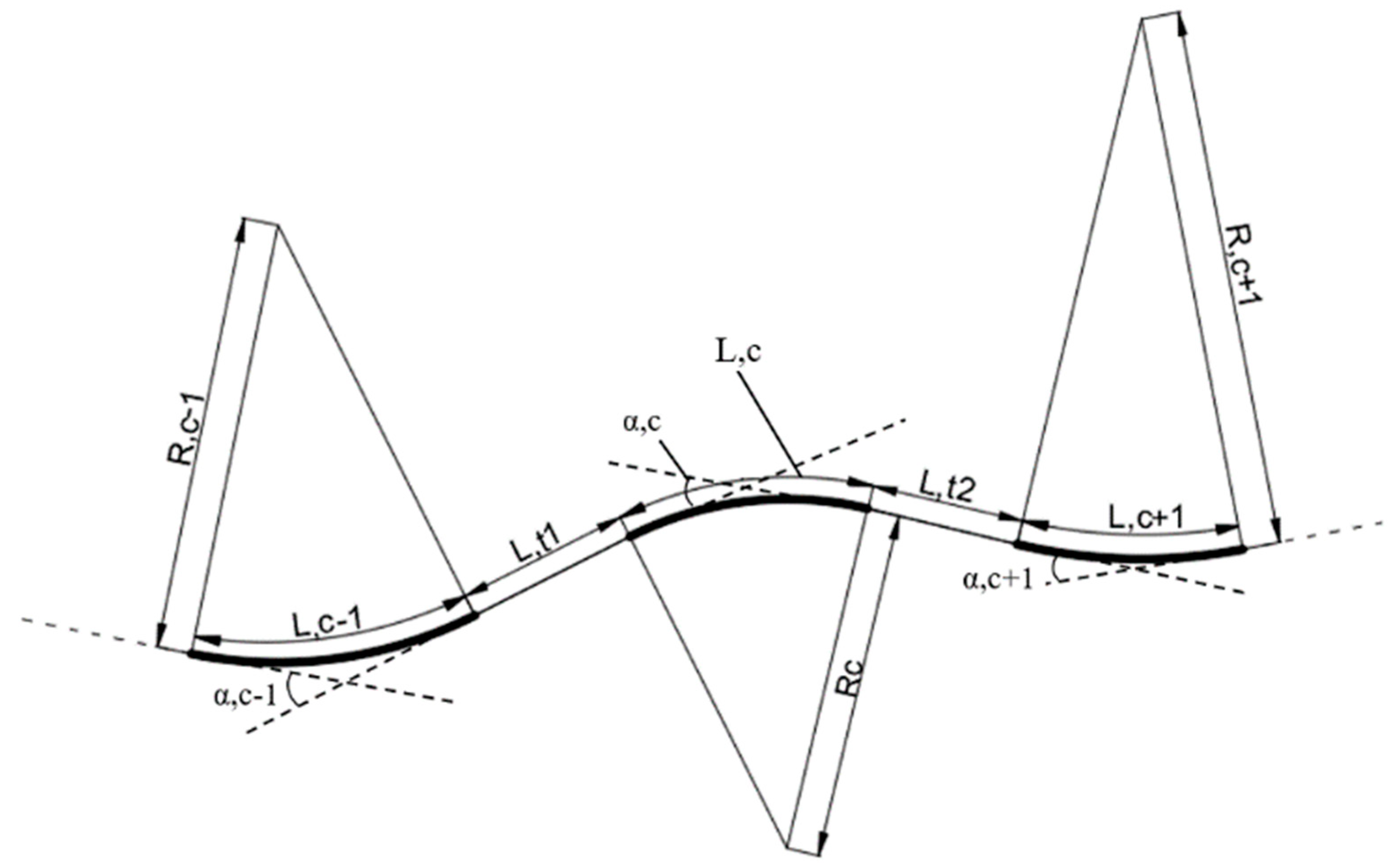
2.2. Geometric Characteristics of the Selected Road Sites

Once road segments including the curved ROR crash sites were identified, their geometric characteristics were collected. This operation was manually conducted by means of on-line sources (i.e., mainly Google Earth^® and Street View^®, see [21,22]) given the unavailability of consistent datasets of road geometric information (such as those used in [13]).

The following geometric features of road segments were inferred (see Figure 1):

• Radius (“R,c”) of the curve (“C”) at which more than one ROR FI crash has occurred;
• Length of the above defined curve (“L,c”)
• Radius (“R,c+1”) and length (“L,c+1”) of the curve (“C+1”) following the curve “C”;
• Radius (“R,c-1”) and length (“L,c-1”) of the curve (“C-1”) previous to the curve “C”;
• Length (“L,t1) of the tangent (“T1”) included between the curves “C” and “C-1”; and
• Length (“L,t2”) of the tangent (“T2”) included between the curves “C” and “C+1”.

In addition to these measures, the average road width “W,c” at the curve “C” was collected, alongside the average slope “i,c” of the curve “C”, which was estimated through the elevation profile obtained through Google Earth^®. Note that the attributes “previous” and “following” given to the curves/tangents were defined as only based on the order in which they were reconstructed, since the direction of travel of the crashed vehicle was unknown.

Based on these direct measures, other indirect measures of curvature were computed, namely the curvature change ratio (CCR) [23] both for curve “C” and the overall segment, as follows:

$$CCR,c=\frac{\alpha ,c}{L,c}=\frac{63.66}{R,c \left[km\right]}$$

(1)

$$CCR,tot=\frac{{{\displaystyle \sum }}_i{\alpha }_i}{L,tot}=\frac{{{\displaystyle \sum }}_i{\left(\frac{L}{R}\right)}_i}{L,tot}=\frac{{\left(\frac{L}{R}\right)}_{,C-1}+{\left(\frac{L}{R}\right)}_{,C}+{\left(\frac{L}{R}\right)}_{,C+1}}{L_{,C-1}+L_{,C}+L_{,C+1}+L_{,t1}+L_{,t2}}$$

(2)

where

CCR,c = curvature change ratio of the ROR crash curve C [gon/km];

CCR,tot = curvature change ratio of the overall segment [gon/km];

$\alpha ,c$ = angle included between the two tangents preceding and following the curve C [gon];

$\alpha ,i$ = angle included between the two tangents preceding and following a given curve [gon];

L,tot = total segment length [km].

R,_c, R,_c-1, R,_c+1, L,_c-1, L,_c, L,_c+1, L,_t1, and L,_t2 are the measures above specified in this paragraph [km].

It should be noted that it is possible to plausibly reconstruct the geometry of curves without relying on transition curves, and then Equations (1) and (2) do not account for them. Clearly, on one hand, the reconstructions were limited by the use of on-line sources, but on the other hand, the transition curves could actually be absent. In fact, in most cases, the road layouts analyzed were very old and have belonged to the main national network for decades, which could explain the absence of transition curves.

2.3. Operational Characteristics of the Selected Road Sites

Based on the reconstructed geometric characteristics, it was possible to infer the operational characteristics of the 30 selected road segments where these characteristics mainly concerned speeds.

2.3.1. Inferred Operating Speeds

Operating speeds can be computed based on the geometric characteristics through appropriate local models from previous research. The selected road segments belong to the Italian national road network and so Italian operating speed models were searched. Models retrieved in [24,25], namely for two-way two-lane rural road curves and tangents, were selected from the review of operating speed models included in [26]. These models are reported as follows:

$$S_{85,C}=a-b R_{C,i}{}^{-0.5}$$

(3)

$$S_{85,T}=S_{85,Cp}+0.081 L_{T,i}{}^{0.75}$$

(4)

where

$S_{85,C}$ = 85^th percentile of the operating speed at the two-way two-lane rural curve C,i [km/h];

$S_{85,T}$ = 85^th percentile of the operating speed at the two-way two-lane rural tangent T,i [km/h];

$S_{85,Cp}$ = 85^th percentile of the operating speed at the curve C_p previous to the tangent T,i [km/h];

$R_{C,i}$ = radius of curvature of the curve C,i [m];

$L_{T,i}$ = length of the tangent T,i [m];

$a$ = constant [km/h] depending on the CCR computed for the single curve C (see Equation (1)), namely equal to 124.1 (CCR < 30 gon/km), 118.1 (30 ≤ CCR < 80 gon/km), 111.6 (80 ≤ CCR < 160 gon/km), 110.8 (CCR ≥ 160 gon/km);

$b$ = constant [km*m^0.5/h] depending on the CCR computed for the single curve C (see Equation (1)), namely equal to 563.78 (CCR < 30 gon/km), 510.56 (30 ≤ CCR < 80 gon/km), 437.44 (80 ≤ CCR < 160 gon/km), 346.62 (CCR ≥ 160 gon/km).

Equations (3) and (4) were used in this study to compute the speeds at tangents and curves of the investigated road segments, based on their geometric characteristics. Note that the inferred 85^th operating speed was deemed more informative than the posted speed limits since: (a) the maximum speed limit on this Italian specific road category is 90 km/h, but the geometric characteristics may compel drivers to lower speeds; (b) no fixed speed control enforcement systems were noted on the segments, mainly located in sparsely populated rural areas; and (c) in several cases, it was not possible to associate a specific posted speed limit to the road sections analyzed.

2.3.2. Inferred Design Speeds

Operating speeds (measured through their 85^th percentiles, as in Equations (3) and (4) may suggest the actual speed that is not exceeded by 85% of drivers at a given curve or tangent, based on their geometric characteristics. If the operating speeds are much higher than the design speeds for each road element, this may result in a safety issue [5,20,27]. This is particularly relevant for curves, for which high speeds may result in not meeting equilibrium conditions. For this reason, in this study, the difference between curve operating and design speeds was investigated.

The theoretical curve design speeds can be inferred from standard equilibrium considerations:

$$R_C={\frac{S_{D,Ci}{}^2}{127\ast \left(q\left(R_{C,i}\right)+ f_t\left(S_{D,Ci}\right)\right) }}_{}$$

(5)

where

$S_{D,Ci}$ = inferred design speed for the curve C,i [km/h];

$R_{C,i}$ = radius of curvature of the curve C,i [m];

$q\left(R_{C,i}\right)$ = cross slope (superelevation) of the curve C,i, usually set as a function of $R_{C,i}$[-];

$f_t\left(S_{D,Ci}\right)$ = side tire-pavement friction coefficient at the curve C,i, which depends on several variables and is usually assumed as varying with vehicle speed $S_{D,Ci}$ at curve C,i [-].

The inferred design speed obtained by inverting Equation (5) is equal to the maximum speed allowed for a given radius under given friction coefficients and cross slopes. Hence, for existing roads (see [5,27]), if operating speeds are higher than the design speeds inferred based on their geometric characteristics, a safety issue can be highlighted. In this study, this comparison was conducted for both ROR crash curves and adjacent non-ROR crash curves, to reveal potential differences. Since the direction of travel of the crashed vehicle is not known from the dataset, differences were searched between the crash curves and the adjacent (previous/following) curves through averages.

It should be pointed out that Equation (5) is internationally used in the practice of road design. However, both relationships $q= q\left(R_C\right)$ and $f_t=f_t\left(S_{D,C}\right)$ actually vary between countries (see [28]) as well as the maximum values for cross slopes (e.g., 0.07 for Italy [29], 0.08 for the United States [30], and 0.10 in local Australian guidelines [31]). Since the curves on Italian two-way two-lane national road network were analyzed in this study, those relationships were developed according to the Italian standards [29] for the relevant road type, and are reported as follows:

$$f_t\left(S_{D,C}\right)=k_1 S_{D,C}{}^2-k_2 S_{D,C}+k_3$$

(9)

where

$R_{C,i}, q\left(R_{C,i}\right), S_{D,Ci}$ has been previously defined with the inferred $S_{D,Ci}$ computed according to Equation (5). Note that for new projects, the design speed of all of the road layout elements should be included between 60 km/h and 100 km/h, according to the reference Italian standards [29], but this was not considered since design speeds were here inferred for existing roads;

$R_{q,min}$ = minimum radius for which the minimum cross slope $q_{min}$ is implemented;

$R_{q,max}$ = maximum radius for which the maximum cross slope $q_{max}$ is implemented;

$k_1, k_2, k_3$ = coefficients of the regression curve obtained based on the values suggested: (a) in the Italian standards in case of wet pavements, (b) in [27,32] in the case of dry pavements. (c) In the case of icy pavements, $f_t$ was assumed to be constant in the range of possible values: $k_1$ = $k_2$ = 0, $k_3$ = 0.10 (see e.g., [33]). Note that dry and icy coefficients are not mentioned in the Italian standards [29] and so they were otherwise determined.

The application of Equations from (6) to (9) to Equation (5) provides the following Equation (10):

$$S_{D,Ci}{}^2\left(\frac{1}{127R_{C,i} }-k_1\right)+k_2 S_{D,Ci}-\left(q\left(R_{C,i}\right)+ k_3\right)=0$$

(10)

where all the terms have been previously defined. The solution of Equation (10) provides the inferred design speed $S_{D,Ci}$ for a given radius of curvature according to the values imput for the triad of coefficients $k_1, k_2, k_3$, previously defined for dry, wet, and icy conditions, respectively. The crash dataset analyzed included information on the pavement conditions at the moment of the crash (i.e., dry, wet, or icy). Hence, it was possible to compute a design speed value for each pavement condition at each crash site where relevant (e.g., using wet coefficients in case of crashes on wet pavements at a given site).

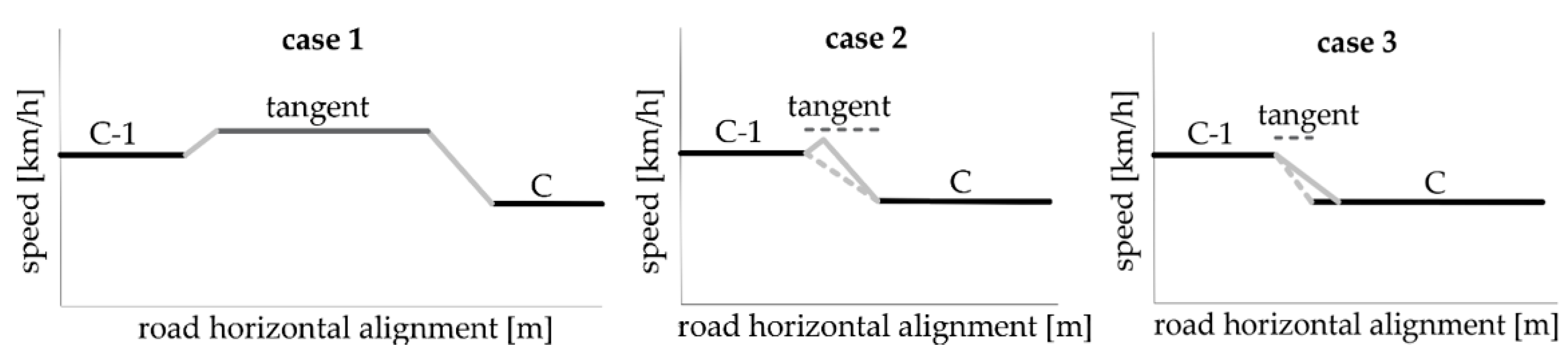
2.3.3. Acceleration Rates

The inferred operating speeds were also used to compute acceleration/deceleration rates in approaching/departing from curves for the curves at which ROR FI crashes occurred. Instead of relying on single constant values, acceleration/deceleration rates were computed based on local acceleration models such as in the case of operating speeds. In this case, experimental models retrieved in [24] were selected from the review of acceleration models included in [26], which relate the acceleration/deceleration rates [m/s²] (namely AR and DR) to the radius of curvature $R_{C,i}$ [m]:

$$AR,i=1.328-0.159\ln R_{C,i}$$

(11)

$$DR,i=1.757-0.222\ln R_{C,i}$$

(12)

Based on the accelerations/decelerations inferred from the above defined equations for each curve, it is possible to compute the necessary lengths for the acceleration/deceleration to occur, in other words, for accelerating after the curve (to the following tangent speed based on Equation (4)) or decelerating before it (starting from the previous tangent speed, Equation (4)). In some cases, it could also be possible (e.g., in the case of short tangents included between a sharp and a larger radius of curvature) that the previous tangent speed is lower than the inferred following curve speed. In this case, an acceleration is likely to occur before the curve, rather than a deceleration.

The acceleration/deceleration lengths can be easily computed as follows:

$$L,a=\frac{0.077 (S_0^2-S_1^2)}{\pm 2 a}$$

(13)

where

L,a = length of acceleration/deceleration [m];

$S_0^{}$= initial speed [km/h];

$S_1^{}$= final speed [km/h];

a = acceleration (AR, computed from Equation (11)) or deceleration (DR, computed from Equation (12)) [m/s²], in the case of deceleration, the minus sign is considered.

Based on the computed lengths through Equation (13), three cases can occur (see Figure 2):

• The tangent before the crash curve C can include both the previous curve-to-tangent acceleration length and the tangent-to-curve C acceleration/deceleration length;
• The tangent before the curve C is not long enough to include both the previous curve-to-tangent acceleration length and the tangent-to-curve C acceleration/deceleration length; and
• The tangent before the curve C is so short that it cannot even include the tangent-to-curve C acceleration/deceleration length.

In both cases 1 and 2, the assumptions about the acceleration/deceleration rates computed through Equations (11) and (12) are reasonable: there is enough space for the driver to accelerate/decelerate through these rates. However, in the second case, since there is not enough space on the included tangent for two acceleration/deceleration phases (from the previous curve to the tangent, and from the tangent to the curve C), a single acceleration/deceleration phase is considered, depending on the difference between the subsequent curve speeds (Figure 2). In the case of curve C with a speed less than the previous curve speed, a single deceleration phase (DR depending on curve C, Equation (12)) is considered. In the opposite case, a single acceleration phase is considered (AR depending on curve C-1, Equation (11)).

In the third case instead, assuming the computed AR/DR (Equations (11) and (12)) as a reference is misleading, since an adequate tangent length is not available (assuming constant speeds in curves). Only in this case, the corrected actual AR/DR are computed by inverting Equation (13), as follows:

$$\pm a=\frac{0.077 (S_{C-1}^2-S_C^2)}{2 L_T}$$

(14)

where all the terms were previously defined (in this case, the initial speed is the previous curve speed, the final speed is the curve C speed, and the length L_T is the tangent length).

Note that the acceleration/deceleration rates and the related relationships are independently computed for both directions of travel for the sake of obtaining a complete portrait of acceleration/deceleration behaviors at curves. This means that the three cases depicted in Figure 2 were taken into account for both directions of travel.

2.4. Safety Measures of Selected Road Sites

Finally, safety indicators were computed for the curves included in the selected road sites. The selected indicators were two crash modification factors (CMFs) for horizontal curves on two-way two-lane rural roads: the first included in the Highway Safety Manual (HSM) [19] (based on [34]), considering the absence of spiral transition curves in Equation (15), and the second provided in [12] (adapted from the original source in Equation (16), considering the presence of curves and the CCR measure). These can be reported as follows:

$$CMF,i \left(HSM\right)=1+\frac{80.2}{1.55\ast R_{C,i}\left[ft\right]\ast L_{C,i}\left[mi\right]}=1+\frac{25380.9}{R_{C,i}\left[m\right]\ast L_{C,i}\left[m\right]}$$

(15)

$$CMF,i \left(Gooch et al. 2016\right)=\exp \left(0.053+0.001479 CCR\right)$$

(16)

where all the terms have been previously defined.

The computation of the CMF for both curves with ROR FI crashes and adjacent curves with no ROR FI crashes was performed in order to reveal significant differences.

3. Results and Discussion

Results obtained from the analysis are reported and discussed as follows, according to the main research questions posed in the introduction. The typical features of ROR crashes occurring at curves of two-way two-lane rural roads segments and the recurrent road geometric and operational characteristics of these ROR FI highly-prone segments are shown. The way in which these aspects could be useful from a road safety management perspective will also be discussed.

3.1. Typical Features of Run-Off-Road Fatal+Injury Crashes

On the curved road sites identified, 69 ROR FI crashes occurred during the observation period (2.3 ROR FI crash/curve, maximum: 5, minimum: 2). Those crashes resulted in 85 injuries (1.23 per crash, 2.83 per curve), and four deaths (0.06 per crash, 0.13 per curve). Moreover, an additional six ROR FI crashes recorded at curves adjacent to the crash C curves were included in the study segments.

The typical features of the ROR FI crashes that occurred at the road curves analyzed are reported in

Table 1. Run-Off-Road Fatal+Injury specific crash features at the selected two-way two-lane rural road curves with statistics averaged over the total crashes (69) and total curve sites (30).

Crash Features	Classes of the Crash Features
Period of the day	Morning	Afternoon	Evening	Night
Per crash	21 (0.30)	34 (0.49)	6 (0.09)	8 (0.12)
Per curve site
(most frequent class per site) 1	3 (0.10)	10 (0.33)	0 (0.00)	3 (0.10)
(most frequent together with others) 2	14 (0.47)	21 (0.7)	4 (0.13)	5 (0.17)
Pavement conditions	Dry	Wet	Icy
Per crash	29 (0.42)	38 (0.55)	2 (0.03)
Per curve site
(most frequent class per site) 1	9 (0.30)	12 (0.40)	0 (0.00)
(most frequent together with others) 2	17 (0.57)	20 (0.67)	2 (0.07)
Vehicle	Auto	Motorcycle	Heavy vehicle
Per crash	47 (0.68)	14 (0.20)	8 (0.12)
Per curve site
(most frequent class per site) 1	16 (0.53)	4 (0.13)	1 (0.03)
(most frequent together with others) 2	25 (0.83)	8 (0.27)	6 (0.20)
Contributory factor	Speeding	Distraction	Avoiding strike	Missing
Per crash	29 (0.42)	29 (0.42)	5 (0.07)	6 (0.09)
Per curve site
(most frequent class per site) 1	8 (0.27)	8 (0.27)	2 (0.07)	0 (0.00)
(most frequent together with others) 2	15 (0.50)	20 (0.67)	3 (0.10)	4 (0.13)
Driver age	Young: 18–29	Adult: 30–64	Over 65	Missing
Per crash	15 (0.22)	46 (0.67)	7 (0.10)	1 (0.01)
Per curve site
(most frequent class per site) 1	2 (0.50)	14 (0.67)	0 (0.10)	0 (0.00)
(most frequent together with others) 2	10 (0.33)	28 (0.93)	5 (0.17)	1 (0.03)

¹ Quantifies in how many curves the specific class of the crash feature was the most frequent by also presenting the percentage over all curves (e.g., in three sites out of 30 (10% of sites), morning crashes were the most frequent). ² Quantifies in how many curves the specific class of the crash feature was the most frequent together with the others (i.e., the most frequent feature shared between two or more classes given the small amount of data) by also presenting the relative percentage over all curves (e.g., in 14 sites out of 30 (47% of sites), morning crashes were the most frequent or the most frequent together with other periods such as evening/night).

, with specific regard to the period of the day, the pavement conditions, the vehicle involved in the crash, the main reported contributory factor reported, and the driver age.

Some useful indications can be argued from the data in Table 1. In 14 out of 69 ROR FI curve crashes, the crash occurred during the evenings or nights (21% of all crashes). It is worth noting that at three sites, night crashes were the most frequent (up to five sites if they are considered the most frequent together with other periods). At four sites, evening crashes were the most frequent (together with other periods). This means that at nine sites (30% of all sites), lighting systems could be a serious issue (lack of visibility has been previously linked to these types of crashes [35]), since most evening/night crashes occur at these curves. The percentage of evening/night crashes (21%) was less than the percentage (36%) computed for all traffic crashes that occurred in Italy on all roads (i.e., in 2017, as a benchmark sample). This could be related to the typical features of the investigated segments, which were far from densely populated urban centers with a likelihood of scarce traffic in the evening/night hours.

As expected, most of the ROR FI crashes analyzed occurred in wet pavement conditions. This was the most frequent condition (in some cases shared with other conditions) in 20 sites out of 30. However, this means that several crashes also occurred during dry conditions. The icy pavement condition was very rare (only two crashes out of 69). The percentage of wet pavement crashes (55%) was disproportionate with respect to the benchmark dataset for all crashes, where it was only 13%. This was expected and is coherent with previous research [35,36], given that loss of friction is more likely on wet pavements.

A significant number of ROR FI curve crashes involved motorcyclists. Considering that most of the investigated segments are far from densely populated urban settlements, motorcycle crashes should be even more highlighted (and is actually a well-known issue, see [37]). Moreover, at eight sites, motorcycle ROR FI crashes were the most frequent (together with other vehicles). However, the percentage of motorcycle crashes (20%) was not disproportionate with respect to the benchmark dataset for all crashes (15%). Conversely, there were few crashes with heavy vehicles involved (about 10%), while in other contexts, this was raised as a more urgent problem [38].

Data on contributory factors are considerably important in understanding the crash dynamics, even if they are essentially based on police reports, and in some cases are subjective and/or may be biased. Aside from the “speeding” contributory factor, which was overwhelmingly expected (see [39] or [36] for fatal crashes), the “distraction” factor was also revealed to be important (42% of crashes, the same as speeding crashes). Clearly, defining if the driver was distracted immediately before the crash is a hard task, even based on police reports. However, this is an interesting aspect that is consistent with previous research [35], which will be addressed in more detail. It is paramount that even for distracted drivers, speed could have been a crucial factor: when the curve is noticed, a low speed could have helped in the case of very delayed steering maneuvers, while high speeds could have been detrimental. In this case, it is difficult to make comparisons with the benchmark dataset for all crashes, since the number and the nature of contributory factors may vary in the official statistics by ISTAT [7], according to the crash type. However, note that the percentages for the “distraction” contributory factor and the “speeding/not complying with limits” contributory factor accounted for only 10% and 14% in the benchmark dataset for all crashes, respectively.

Concerning the driver age, there are no particular results to highlight being that the “adult” (30–64 years old) class was the most involved in these crashes. Nevertheless, the number of young drivers involved was noticeable, with 22% of crashes involving drivers aged 18–30. However, this percentage is strictly in line with that estimated from the benchmark dataset for all crashes. Moreover, the small dataset does not allow for investigation into combinations of these factors, but previous research has shown that the ages of different drivers may also be associated with different risk factors for ROR crashes [15].

3.2. Typical Features of Road Segments Including Curves with Notable History of ROR FI Crashes

In this section, the results obtained from the investigation of typical features of segments including curves with a notable history of ROR FI crashes are presented and discussed. The presentation is divided according to the different characteristics investigated: geometric, operational, and safety-related.

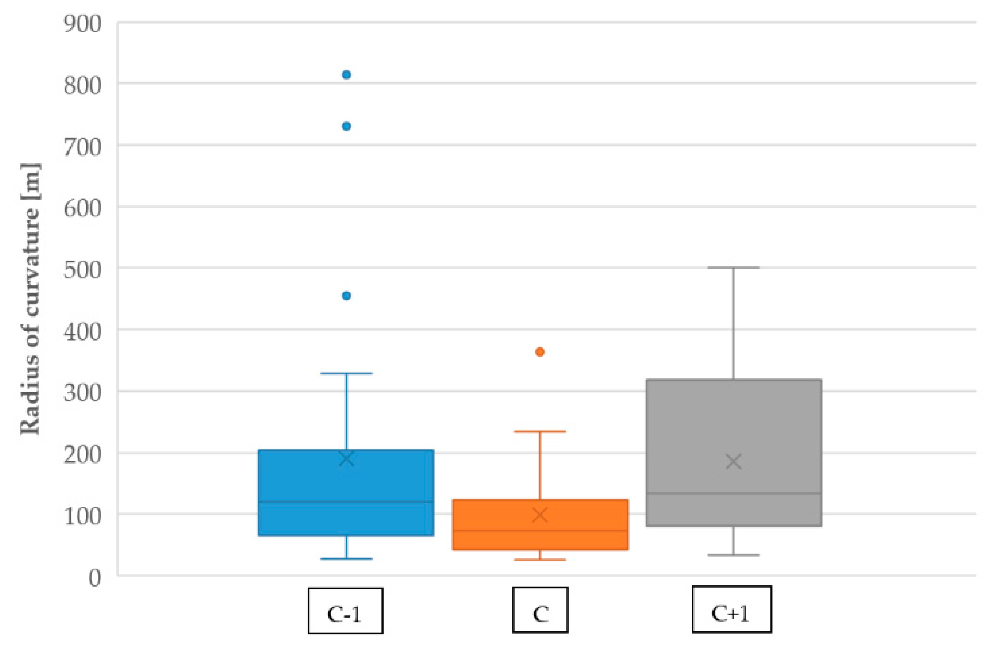
3.2.1. Geometric Characteristics

General results. The 30 road segments analyzed, which included the ROR FI crash-prone curves, were on average 562.9 m long (st. dev. = 461.3 m, max. = 1846.0 m, min. = 175.0 m). A synthetic average measure of their curvature was obtained through the overall CCR (curvature change ratio) of the segment: 380.1 gon/km (st. dev. = 285.9 gon/km, max. = 1250.0 gon/km, min. = 39.6 gon/km). These two measures show a high variability within the sample of segments analyzed: on average, they include three curves in about 600 m, but the standard deviation was not negligible: some segments were extremely short (down to 175 m), while others were very long (up to about 2 km). This means that the possible influence of the lengths of tangents included between the curves on speeds (see [27]) is extremely variable within the segments. A very broad variation of the curvature can also be appreciated: some segments had a negligible curvature compared to their length (down to about 40 gon/km), while for others, the CCR was noticeable (up to about 1300 gon/km).

Hence, further investigations are needed to highlight some common features, besides those used in preliminary measures. More detailed information about geometric features are reported in

Table 2. Descriptive statistics of the geometric features of ROR FI curved crash sites (each statistic is computed over the total number of curve sites: 30).

Crash Curve Geometric Features	Descriptive Statistics
	Mean	St. Dev.	Maximum	Minimum
Radius of curvature Rc [m]	112.3	86.9	364.0	26.0
Length of the curve Lc [m]	93.7	79.3	302.0	24.0
CCR ratio–curve C [gon/km]	924.6	607.2	2448.5	174.9
Length of adjacent tangent 1 [m]	151.7	212.3	1193.0	9.0
Curve road width [m]	7.5	1.2	9.5	4.5
Curve average longitudinal slope [%]	4.0	2.8	12.0	0.0
Mean radius of adjacent curves 1 [m]	190.9	160.3	814.0	26.0
Mean length of adjacent curves 1 [m]	82.9	63.3	299.0	7.0
CCR ratio—adjacent curves 1 [gon/km]	618.5	534.8	2448.5	78.2

¹ Statistics for adjacent curves refer to the average between the following and previous curves to curve C (i.e., curves C-1 and C+1 in Figure 1).

. Synthetic measures were computed for the crash curve C (see Figure 1), which included other geometric information about the analyzed segment (tangents, previous and following curves).

As expected, the average radius of the curvature of the crash curves was sharp (about 110 m on average) and the related standard deviation was relatively small (with a maximum radius of 364 m). This means that there were no large curves (e.g., with a radius > 400 m) in the analyzed sample of the ROR FI crash-prone curves. A similar tendency was noted for the crash curve lengths: on average, curves were only about 100 m long. On the other hand, there was high variability in the average length of the previous/following tangents of about 150 m long, with a standard deviation greater than the mean. Note that the minimum average tangent is about 10 m long (practically negligible, i.e., the tangent could have no effect on speeds, which are mainly governed by the subsequent curves), while the maximum average tangent is more than 1 km long (high speeds can be reached on tangents before curves). The crash curve width is in line with standard measures for two-way two-lane rural roads. However, curve enlargements may be needed for different reasons (i.e., for visibility reasons or to avoid dangerous encroachments of heavy vehicles). Hence, it seems that in several cases (given an average curve width of 7.5 m), enlargements were not present. Note that there were also cases of crash curves on narrow roads (down to 4.5 m). Moreover, it is important to note that most crash curves are on a notably steep longitudinal slope (average of 4%, up to 12%). This could clearly have affected the vehicle dynamics while approaching curves (i.e., while braking in downhill sections).

Furthermore, the measures computed by taking into account the geometric features of adjacent elements provide some additional insights. In detail, the mean radius of adjacent curves was significantly greater than the crash curve radius (about 190 m, with respect to about 110 m). The computed average ratio of the crash curve radius to the average previous/following curve radii was 0.78 (st. dev. = 0.56). However, the mean length of adjacent curves (about 80 m) was comparable with the mean length of the crash curves (about 90 m). The average CCR computed for the adjacent curves was significantly higher than the average crash curve CCR. Considering both the above reported comparisons for the curve radii and lengths, this noticeable difference in the CCR values can be mostly attributed to largely different radii.

In-depth analysis. The qualitatively identified differences between the radii and lengths of the crash curves with respect to adjacent curves on which, on the contrary, no ROR FI crashes have occurred were tested by means of statistical tools. Given that the distributions of both curve radii and lengths do not evidently follow normal distributions, non-parametric tests were conducted. Moreover, the crash curve and the adjacent curves (both the populations of previous and following curves) belong to the same segment. Hence, they were considered as paired measures, thus leading to the selection of the non-parametric Friedman test. The differences between (a) the radii of curvature, and (b) the lengths of the three populations of crash curves C, previous curves C-1, and following curves C+1 were tested. Six adjacent curves to the analyzed crash curves C on which one ROR FI crash had occurred in the observation period were discharged. In this way, differences between the ROR FI crash-prone curves (more than two crashes in four years) and the no-ROR FI crash curves can be captured.

As a result of the tests, there was a statistically significant difference at the 5% significance level in the radius of curvature depending on the curve type (crash/previous/following curve), χ2(2) = 10.126, p = 0.006 (see boxplots in Figure 3). Post-hoc analysis with the Nemenyi test revealed that, as expected, the only statistically significant differences were between curves C/C-1 and C/C+1, and not between curves C-1/C+1. In fact, the boxplots in Figure 3 evidently show that the radius of the curvature of the adjacent curves was higher, on average, than the radius of the curvature of the crash curve. Instead, there was no statistically significant difference in the curve length depending on the curve type (crash/previous/following curve), χ2(2) = 0.083, p = 0.959.

Results from the statistical tests suggest that a significantly different radius of the crash curve with respect to the adjacent curves could have fostered the crash to occur at that specific curve. This was expected from previous research on road design consistency (see [40], with respect to the average radius of the curvature of the road section). Moreover, the homogeneity of the subsequent curve radii is a recommendation/prescription included in several guidelines/standards worldwide [23]. Hence, this result shed additional light on the importance of consistency between adjacent road curves. The opposite trend is also known from previous research: when a curve is included between sharper adjacent curves, its safety performance improves [11,12]. In this study, the lack of consistency was specifically linked to the ROR FI crash frequency occurrence (at least two ROR FI crashes in four years of observation). Hence, it can surely be used as an indicator while conducting a road safety audit or when planning inspections [20], specifically in case of a dedicated safety campaign (e.g., [41]). On the other hand, among other characteristics, it seems that the relationship between the length of adjacent curves and the length of the crash curve is not influential. In practice, the curve minimum length can be set as a function of its speed (and then its radius) [29], but without specifying the relationship between subsequent curve lengths. In this case, if the radii are consistently designed, then the lengths will also be consistently designed as a consequence. Moreover, when checked against Italian requirements [29] for minimum curve lengths (which can be traveled in at least 2.5 s), only two crash curves out of 30 did not meet the minimum requirements. Hence, this can be considered as a minor issue.

Link between geometric and crash features. As previously discussed, the unexpected nature of the curve (i.e., with a significantly sharper radius) can lead to sudden maneuvers with undesired outcomes. Clearly, this process can be further hampered if the driver is distracted or in the case of non-optimal visibility conditions. Given the available data, some further analyses were conducted to investigate this aspect in detail. In fact, the number of crash sites in which (a) most crashes had distraction as a main contributory factor, and (b) the most crashes that occurred during evening/night have been previously defined (see Table 1 for the case of the most frequent together with other factors). Binary logistic regression was used to establish if the average ratio between the crash curve and the average adjacent curves radii could predict: (a) the likelihood of being a “distraction” crash site versus a “non-distraction” crash site, and (b) the likelihood of being a “evening/night” crash site versus a “morning/afternoon” crash site.

As a result of the binary logistic regression, an increase in the percentage ratio (crash curve to adjacent curves radius) was associated with a decreased likelihood (odds ratio = 0.983, p = 0.097) at the 10% significance level of being a site with the most crashes with distraction as a contributory factor. This is highlighted in the boxplots of the ratios of crash curve radii to adjacent radii in Figure 4 for both the “distraction” and “not distraction” crash sites. This result means that, the greater the difference between the crash curve radius and the adjacent curve radii, the more the crash site will be related to “distraction” contributory factors. Distracted drivers, who are driving in an almost unconscious state (see [42]), may be even more surprised than other drivers by an inconsistent radius of curvature with respect to previous curves to which they are used to. This may occur even if distracted drivers are more prone to adapt their speeds at sharp curves (i.e., lower speeds) when compared to other drivers [43]. This finding confirms the crucial relationship between road design consistency and road safety [23,41,44], and the importance of criteria for ensuring geometric design consistency (see [45,46]).

Instead, no statistically significant relationships were found between the curve ratios for evening/night crashes versus morning/afternoon crashes. This means that, even if there is a significant percentage of evening/night crashes, which may indicate visibility issues (fostering ROR crashes, see [35]), the effect of inconsistent curve radii with respect to the adjacent ones is not affected by the day/night condition.

3.2.2. Operational Characteristics

General results. Design and operating speeds were inferred for the 30 curves in the analyzed segments. The results are reported in

Table 3. Descriptive statistics of the operational features of ROR FI curved crash sites (each statistic was computed over the total number of curve sites that met the specific requirements considered).

Curve Operational Features	Descriptive Statistics
	Mean	St. Dev.	Max.	Min.
Dry inferred maximum design speed—curve C [km/h] 1	65.5	20.2	104.6	38.2
Wet inferred maximum design speed—curve C [km/h] 2	54.3	15.6	89.1	33.4
Icy inferred maximum design speed—curve C [km/h] 3	44.4	20.1	58.6	30.1
Dry inferred max. design speed—adjacent curves 4 [km/h]1	77.5	23.8	135.4	39.4
Wet inferred max. design speed—adjacent curves 4 [km/h]2	65.0	19.2	110.7	31.4
Icy inferred max. design speed—adjacent curves 4 [km/h]3	53.8	22.0	85.0	33.8
Dry 85th—max. design speed difference: curve C [km/h]1	−3.5	7.2	2.4	−21.9
Wet 85th—max. design speed difference: curve C [km/h] 2	7.9	4.5	11.7	−6.5
Icy 85th—max. design speed difference: curve C [km/h] 3	16.0	1.8	17.2	14.7
Dry 85th—max. design speed diff.: adjacent curves 4 [km/h] 1	−8.0	12.1	2.4	−46.8
Wet 85th—max. design speed diff.: adjacent curves 4 [km/h] 2	4.5	8.2	11.7	−22.0
Icy 85th—max. design speed diff.: adjacent curves 4 [km/h] 3	13.6	11.2	20.0	−3.2
Deceleration in approaching curve C—both directions [m/s2] 5	−1.6	2.0	-0.4	−9.7
Acceleration in approaching curve C—both directions [m/s2] 6	2.2	-	-	-
Discordant deceleration/acceleration in approaching curve C in the two different directions [m/s2] 7	0.3	2.4	2.4	−2.0

^1,2,3 Design/85^th speed inferred for curves at which at least one crash occurred in (1) dry conditions (21 sites), (2) wet conditions (21 sites), and icy conditions (two sites). ⁴ Statistics for adjacent curves refer to the average between the curves following and preceding curve C. ⁵ In this case, there is deceleration in approaching to curve C in both directions (20 segments out of 30). ⁶ In this case, there is acceleration in approaching to curve C in both directions (one segment). ⁷ In this case, there is acceleration from one direction, and deceleration from the opposite direction (nine segments).

in terms of: (a) the maximum design speeds for both crash curve C and the average adjacent curves (in dry, wet, and icy conditions), (b) the difference between the 85^th operating and maximum design speeds for both the crash curve and the average adjacent curves; and (c) the acceleration/deceleration rates in approaching the crash curve C.

Consistently with the results concerning geometric features, the inferred maximum design speeds for the curve C were lower, on average, than the speeds computed for the adjacent curves. In fact, this basically depends on the different average radius across the two categories of curves. The average maximum design speed at crash curves was 65.5 km/h (st. dev. = 20.2 km/h) in dry conditions and 54.3 km/h (st. dev. = 15.6 km/h) in wet conditions. This means that the equilibrium requirements (Equation (5)) are theoretically met if those speeds are not exceeded in the respective pavement condition (dry/wet). However, if ROR crashes occurred at those curves, then it is likely that those speeds were actually exceeded. There are some cases in which the inferred maximum design speed was very high and could not be clearly realistic (e.g., the max. dry speed = 135.4 km/h). In these cases, it is likely that some other aspects could have contributed to the crash besides that of only speeding (e.g., distraction, see Table 1). However, even if other factors were determinants, speed is still a crucial factor; if adequate speeds were operated, then a recovery maneuver could have possibly led to avoiding the crash. While similar remarks are valid for icy conditions, this is not further discussed since they only were found at two sites.

In dry conditions, the average inferred 85^th operating speed was lower, but comparable (−3.5 km/h) with the maximum design speed on the crash curve and even significantly lower (−8.0 km/h) than the maximum design speed on the adjacent curves. Clearly, according to the standard deviation values, there were several cases in which the 85^th operating speed was higher than the maximum design speeds. However, in dry conditions, the inferred 85^th operating speed values did not provide enough clear evidence that the drivers’ speeds could have been higher than the maximum design speeds for those curves, even if they were comparable. On the other hand, in wet conditions, the average inferred 85^th operating speed was significantly higher (+7.9 km/h) than the maximum design speed on the crash curve as well as on the adjacent curves (+4.5 km/h). Moreover, considering the values of the standard deviations, in the case of crash curves, most of the operating speeds were consistently higher than the inferred maximum design speeds. However, operating speed models are usually estimated considering good weather conditions and are not applicable to the case of wet conditions, even if previous research has shown that the difference can be not significant [47]. It is also important to note that, if compared with a commonly used method for evaluating the safety of two-way two-lane rural roads [23,27], a difference between the operating and design speed of less than 10 km/h (as found here, on average) should not indicate safety issues.

The most interesting result concerns the deceleration rates. In most cases (20 segments out of 30), based on the operating speeds computed for the geometric elements of the analyzed segments, a deceleration is likely to occur in approaching the crash curve from both directions. The average deceleration rate was −1.6 m/s² (max. = −9.7 m/s²), which is higher than the average deceleration rates closer or smaller than the −1 m/s² found in previous research (e.g., [48,49]) and considered in the standards and guidelines (e.g., [29]). It should be pointed out that:

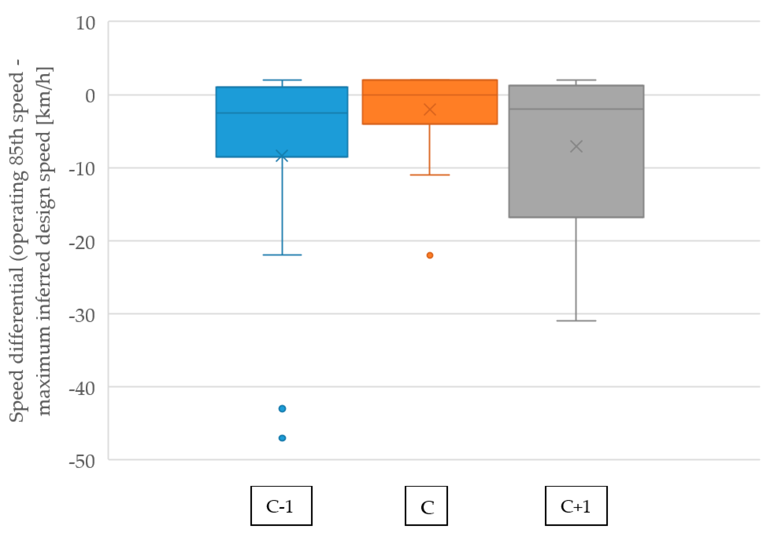
• In eight cases, the length of the tangents included between the crash and adjacent curves were sufficient for both acceleration from the previous curve and further deceleration to the considered curve, with the AR/DR rates computed through Equations (11) and (12) (case 1, Figure 2).
• In seven cases, both the previous and following tangent lengths were insufficient (based on Equation (13) for a proper deceleration computed through Equation (12) to occur, and assumed to possibly occur on tangents only (an experimentally verified usual condition [48]). In cases of insufficient tangent length (case 3, Figure 2), the deceleration rate was computed through Equation (14).
• In all other cases, the length of tangents between the crash curve and the adjacent curves were not sufficient for both acceleration from the previous curve and deceleration to the crash curve to occur (case 2, Figure 2). Hence, in this case, only the deceleration from the previous curve was computed (hypothesis of no acceleration).

These results indicate that, even more than the possible incorrect speed at curves (i.e., higher than the maximum allowed), the sequence of curves implies severe decelerations that may have caused skidding in approaching the curves. The increase in the average degree of variation of operating speeds was actually related to an increase in the expected crash rate in previous research [44]. Moreover, considering that wet conditions were the most frequent for crashes, the role of tire-wet pavement friction in the case of hard braking could have been crucial. Conversely, previous research has shown the positive effect of short tangents between subsequent curves on crashes on the following curve [12,50]. However, these tangents are not entirely comparable: the average distance between the curves in [12] was about 300 m, while in this study, it was about half that (150 m). Hence, the issue pointed out in this study is technically different: very short tangents included between curves having largely different radii may be of particular concern for ROR FI crashes due to the severe decelerations implied.

In-depth analysis. Statistical tests were also conducted for the operational features. In detail, speed differentials (85^th operating—maximum inferred design speed) at crash curves were compared with those at adjacent curves on which, in contrast, no crashes have occurred. Given that the distributions of these speed differentials also do not evidently follow normal distributions, non-parametric tests were conducted. Moreover, they were considered as paired measures (such as in the previous case of geometric features), thus leading to the selection of the non-parametric Friedman test. The differences between (a) the speed differentials (85^th operating—maximum inferred design speed) in dry conditions and (b) the speed differentials in wet conditions of the three populations of crash curves C, previous curves C-1, and following curves C+1 were tested.

As a result of the tests, there was a statistically significant difference at the 10% significance level in the speed differential in dry conditions depending on the curve type (crash/previous/following curve), χ2(2) = 5.943, p = 0.051 (see boxplots in Figure 5). Post-hoc analysis with the Nemenyi test revealed that, in this case, the only statistically significant differences were between crash curves C and previous curves C-1. Instead, there was no statistically significant difference in the speed differential in wet conditions depending on the curve type (crash/previous/following curve), χ2(2) = 3.930, p = 0.140.

Results from the statistical tests showed that there was a significant discrepancy in the speed differential (85^th operating—maximum inferred design speed) between the crash curves and adjacent curves only in the dry condition. The previously discussed general results showed that, in general, the speed differentials are greater on the crash curve than on the adjacent curves in both dry and wet conditions. However, this difference seems noticeable only in the dry condition. This confirms that the 85^th operating speed at the crash curve is comparable with the maximum design speed at the same curve, while it is significantly lower than the maximum design speed on adjacent curves. Hence, drivers who are selecting speeds based on geometric characteristics of adjacent elements, with enough safety margins in dry conditions (average margin of the 85^th speed from the maximum inferred design speed = −8.0 km/h) may continue to rely on their speed selection process even at the crash curve, where the safety margin is significantly lower (on average = −3.5 km/h). This could be crucial for the crash outcome if combined with other potential crash contributing factors (such as the previously discussed distraction issue). The practical implication of this involves being more cautious in interpreting the margins between the 85^th and design speed (e.g., the <10 km/h margin indicated as good design practice [23,27]) for the specific case of ROR FI crash-proneness.

In wet conditions, the populations of speed differentials were similar between the crash curve and the adjacent curves, and average 85^th operating speeds were consistently higher than the maximum inferred design speeds. Hence, there were no particularly evident differences between the crash curve and the adjacent curves, which may suggest that using this speed differential parameter is influential in the crash occurrence at that specific curve. In fact, if aggressive drivers consistently select speeds as suggested by the geometric characteristics, they would surely be in danger of ROR crashes at all curves along the analyzed segment in wet conditions. Hence, on the crash curve, there should be other contributory factors that may have fostered the crash to occur.

3.2.3. Predicted Safety Characteristics

Crash modification factors (CMFs), which were chosen as indicators of the predicted safety characteristics, were computed for both the crash curves and adjacent curves. These are synthetic parameters that may express the crash risk of given curves, based on both their length and radius of curvature (see Equations (15) and (16)). Descriptive statistics on their computed values are reported in

Table 4. Descriptive statistics of the predicted safety features of ROR FI curved crash sites (each statistic was computed over the total number of curve sites (30)).

Crash curve Predicted Safety Characteristics	Descriptive Statistics
	Mean	St. Dev.	Max	Min.
Crash Modification Factor—curve C—Equation (15) [-]	8.6	7.8	36.3	1.2
Crash Modification Factor—adjacent curves 1—Equation (15) [-]	7.3	8.6	39.6	1.1
Crash Modification Factor—curve C—Equation (16) [-]	6.5	8.1	39.5	1.4
Crash Modification Factor—adjacent curves 1—Equation (16) [-]	4.3	6.8	39.5	1.2

¹ Statistics for the adjacent curves refer to the average between the following and previous curves to curve C.

.

It is possible to note that the CMFs for crash curve C were higher, on average, than the CMFs for adjacent curves, especially in the case of the CMFs computed according to Equation (16), where they were evidently larger. However, the standard deviation was high, suggesting an overlap of the two CMF populations, especially for the Highway Safety Manual (HSM) CMF (Equation (15)). A Friedman test conducted on the three populations of CMFs (curves C, C-1, C+1) revealed no statistically significant differences for the HSM CMF (χ2(2) = 0.083, p = 0.959). The same test conducted on the other CMF (Equation (16)) instead revealed statistically significant differences at the 5% significance level (χ2(2) = 10.564, p = 0.005) with the Nemenyi post-hoc test indicating differences between curves C and the following curves (5% significance level). In addition, in these tests, six adjacent curves on which a ROR FI crash occurred were excluded to highlight the differences between high-risk curves and no-crash curves.

First, both CMFs were for the total crashes. This means that, based on the high average CMF values, most of the curves analyzed in this study (both crash and adjacent curves) could be at risk of crashes (CMFs indicate the relative number of crashes compared to straight sections), but that these crashes are not necessarily fatal + injury (FI) and/or ROR. Depending on the local statistics and injury scales, the FI crashes are usually only a small percentage (i.e., around 17% including only severe injuries in [19] for the same road category). This means that, based on CMFs, property-damage-only crashes could have occurred even on the adjacent curves at which ROR FI crashes did not occur in the same period. Moreover, CMFs were developed by using American data and the transferability of CMFs to other countries is not straightforward [8]. Note that an average CMF for horizontal curves that also includes European countries (but not Italy) can be found in [8], even if it is referred to as the base condition of a curve with R = 1000 m (and not to tangents). However, its application would have revealed significant differences between the ROR FI and no-ROR FI crash curves as well as the CMF in Equation (16) [12].

It is important to note that the CMF from Equation (16) outperformed the HMS CMF (Equation (15)) in highlighting sites that may have potential for skidding proneness (with a relevant history of ROR FI crashes). Hence, this CMF, which only depends on the CCR value, could be used to identify high-risk ROR FI crash curves in the network screening stage (at least based on the analyzed data).

3.3. Practical Implications for Road Safety Management

In this section, the results presented and discussed in the previous sub-sections are used to define their practical implications for road safety management purposes. Moreover, some practical design aspects are also discussed that are useful for safety interventions at similar sites.

3.3.1. Recurrent Features Useful for Road Safety Management

Based on the findings from this study, a list of features to be used as indicators of ROR FI crash-prone rural two-way two-lane curves was proposed. These features can be used during the network screening stage (typically conducted by highway agencies or public entities) to highlight some sites that should be studied in more detail (e.g., for on-site inspections or safety-based management). In particular, in this specific case, network screening can be aimed at reducing specific type of crashes such as run-off-road FI crashes. In the following list, only the elements that are immediately available to practitioners are included, considering a scenario in which some sites should be analyzed in more detail in a large road network managed by the same agency. These features are:

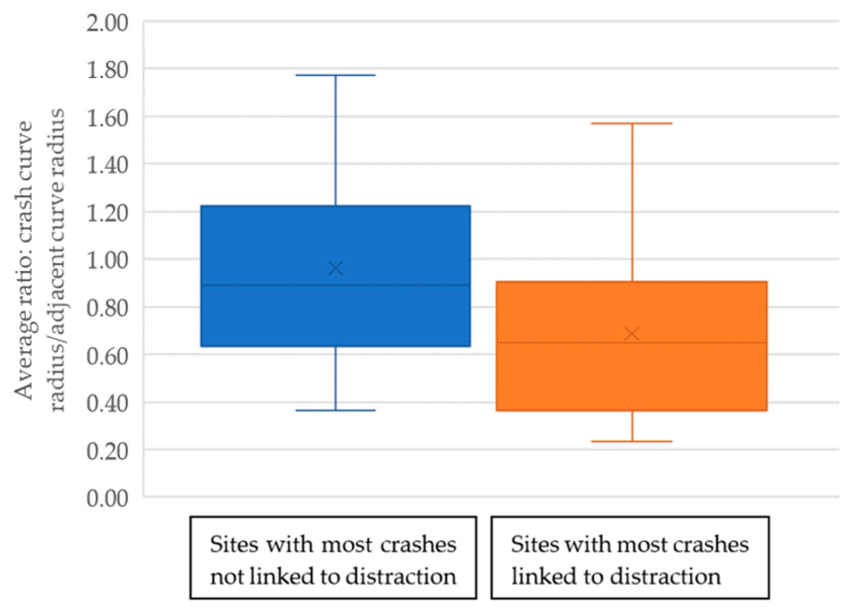
• The ratio between the curve radius and the radius of the adjacent curves (average between the previous and the following curves, since the road type is two-way operated). In this study, by excluding the adjacent curves on which the ROR FI crashes occurred, the average ratio between the crash curve radius and the average adjacent curve radius (on which ROR FI crashes did not occur) was equal to 0.59 and the 85^th percentile of the distribution of ratios for the crash curves was 0.76. Hence, for road safety management purposes, two-way two-lane rural curves with

  $$R_C\le \left(0.59÷0.76\right)\ast \left(\frac{R_{C+1}+R_{C-1}}{2}\right)$$

  (17)

  could be targeted for further investigation while conducting campaigns dedicated to preventing ROR FI crashes on two-way two-lane rural road curves. The choice between the two values proposed (the mean and the 85^th percentile) may depend on the capability for planning further investigations (e.g., inspections) at curves. The CMF (Equation (16) [12]), which has been demonstrated to have the capability to highlight ROR FI crash sites, only depends on the CCR. Hence, a suggested measure based on the difference in CMFs would have been redundant, having already provided the above described relation in Equation (17).
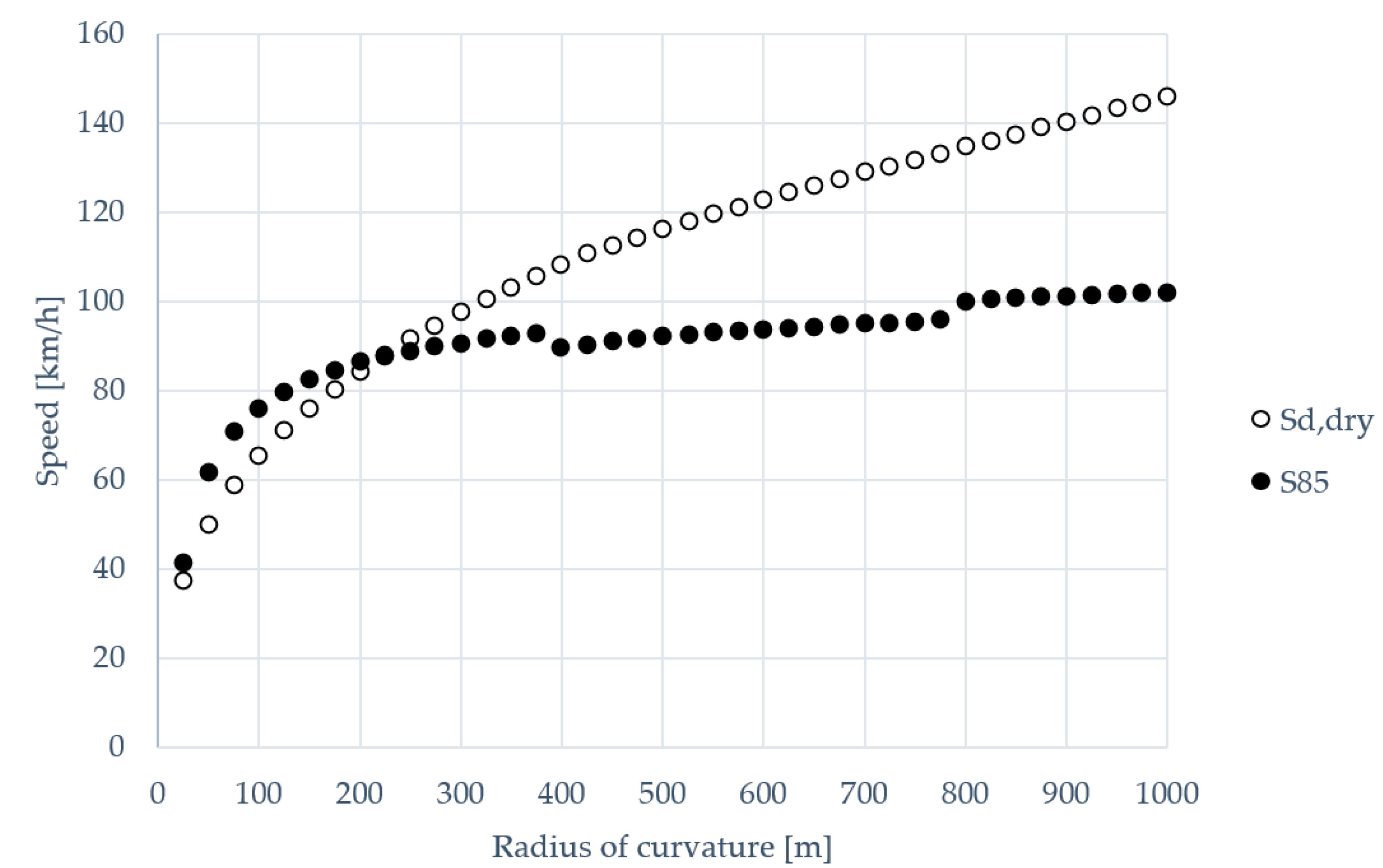
• The difference between the operating speed and design speed in dry conditions. In dry conditions, an inferred operating speed significantly close to the maximum inferred design speed (average margin of −3.7 km/h) was found to be associated with ROR FI crashes at curves. In Figure 6, Equation (3) (85^th inferred operating speed) and Equation (10) (max. inferred design speed) are solved. Given the findings from this study, the radii of curvature for which the 85^th operating speed is greater or closer than the maximum inferred design speed could be targeted for further investigation. In this case, the threshold can be set to around 250 m (close to the intersection between the two curves in Figure 6 and roughly corresponding to the same average margin found in this study). This indication is more conservative than using the conventional 85^th-design speed margin of +10 km/h [23,27] as a threshold, which would correspond to curves with a radius of less than around 150 m, as based on Figure 6.
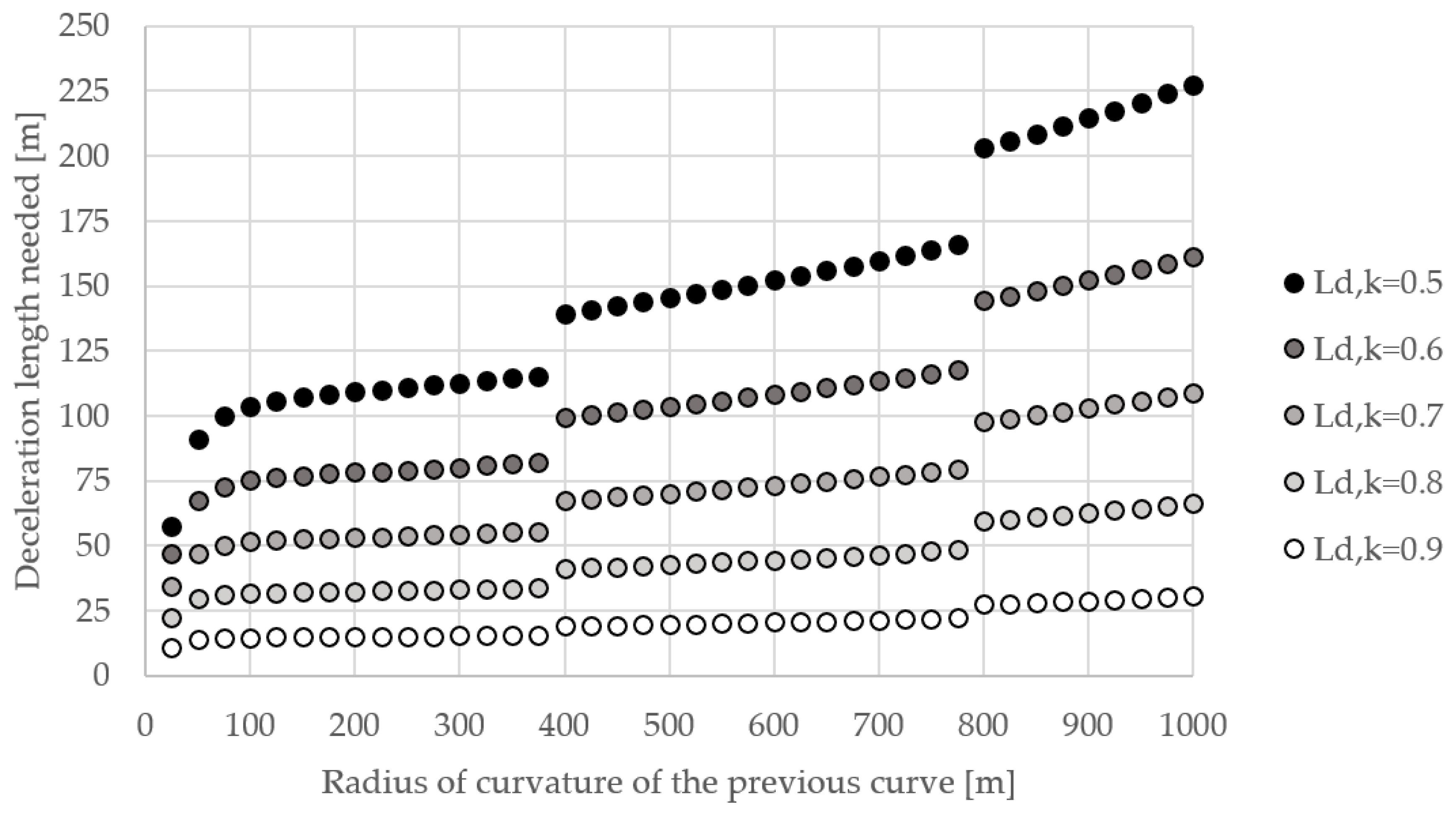
• Deceleration rates. High inferred deceleration rates were found to be associated with ROR FI crash curves. This clearly points out that the length of the tangent included between two subsequent curves (with largely different radii) plays a crucial role. Hence, if the tangent length does not allow a deceleration compatible with Equation (12) (i.e., the tangent is shorter), then tangents before curves with a radius of curvature sharper than the previous ones should be targeted for further investigation. A practice-ready abacus is graphically depicted in Figure 7 and provides the minimum length of the tangent set as equal to the minimum deceleration length needed from the previous curve (with larger radius) to the following curve (with sharper radius). This can be used starting from the radius of the previous curve and by reading the value of the necessary tangent length for different k values (ratio between the radii of the following and previous curve). Tangents that do not satisfy this minimum criterion should be targeted for further investigation during the network screening stage.
• Longitudinal slope. This was highlighted as a critical factor for ROR FI crashes at curves: the average slope was 4.0% in the study sample. This suggests that, as expected, curves on steep slopes should certainly be targeted for further investigation. No further detailed indications are provided in this study since the vertical alignment was considered to a minor extent, given the available data sources and the need for accurate data.

3.3.2. Remarks for Safety Countermeasures on Similar Sites

Based on both the findings from this study and the remarks made in the previous sub-section, a discussion about possible countermeasures on two-way two-lane ROR crash-prone curves is provided as follows.

Basically, the possible countermeasures can be differentiated into long-term and short-term measures, and different sets of countermeasures can be implemented to optimize safety maintenance interventions [5]. Long-term measures typically involve re-designing the road alignment to strictly adhere (or tend to) the current regulations/guidelines (i.e., meeting requirements for radii and transition curves). In several cases, this is not feasible and thus alternative short-term measures can be implemented in some cases specifically dedicated to the ROR crash type (e.g., [41]). The elementary short-term measures that can help in this specific case are:

• Speed reducing measures. Clearly since speeding was indicated as a crucial contributing factor, the importance of reducing speed is paramount. This can be effectively achieved through transverse rumble strips [51] and traffic speed control (e.g., [52]).
• Perceptual measures. It was extensively shown how the mis-perception of the crash curve or the drivers’ distraction could have played an important role in the analyzed crashes. Hence, measures such as curve delineation, warning signs, and sequential flashing beacons can effectively reduce crashes [53] by acting on the drivers’ perceptual mechanism.
• Physical improvements. It is paramount that one of the most frequent ROR FI crash mechanisms is the loss of friction (i.e., when the friction demanded exceeds the available friction [9,10]). A design friction coefficient varying with speed was assumed in the calculations made throughout the paper, since no direct measurements were available. However, considering drivers travelling at the inferred 85^th operating speeds in sharp radii curves (higher than then maximum inferred design speeds, see Figure 6 for R shorter than about 225 m), the friction used is higher than the friction computed in the case of design speed. The actual friction used can be computed through the following equation (obtained by rearranging Equation (5), where q = q_max = 0.07 due to the assumed sharp radii):

  $$f_t\left(S_{85}\right)=\frac{S_{85}{}^2}{127\ast R_C }-q_{max}{}_{}$$

  (18)
  The cross friction coefficients used (light grey dashed line in Figure 8) were significantly higher than the design cross friction coefficients in wet conditions (black dashed line in Figure 8). In fact, a threshold for indicating an unacceptable design condition could be a difference between the used and design cross friction coefficients of more than 0.04 [23,27]. This means that treatments for improving skid resistance should be implemented where there is noticeable evidence that this condition could occur, especially in the case of sharp radii. Another solution could be an increase in the cross slope (superelevation) up to 10% (as suggested in particular cases, e.g., in [31]). In this case, no skid resistance treatments are needed (that is, still assuming the design cross slope is valid) and can be applied to radii of curvature roughly down to 300 m (see black solid line in Figure 8) where q = 0.10 is reached. However, a similar treatment should be considered with extreme cautiousness, especially in the presence of notable vertical grades and possible icy pavements. In fact, the compound slope is often limited by design guidelines, thus resulting in the unfeasibility of implementing cross slopes equal to 10%. Finally, considering the implementation of both increased superelevation and skid resistance treatments does not dramatically reduce the need for increased available friction, especially for very sharp radii (compare dashed light grey line with dashed grey line in Figure 8).

4. Conclusions

In this study, Italian two-way two-lane rural road curves on which more than one ROR FI crash in the observation period of five years occurred were analyzed. The aims of the study were: (a) the identification of recurrent specific features for ROR FI crashes at curves of the road type analyzed, (b) the identification of recurrent specific geometric and operational features that may be associated with the occurrence of ROR FI crashes at curves, and (c) link empirical findings from the study to road safety practice. These research questions were addressed through a micro-analysis approach involving accident reconstructions [16,17,18,39], which allowed for additional insights than traditional macro-level approaches (e.g., [2,54]).

The following conclusions can be drawn based on the research questions:

• There were some recurrent features in the ROR FI crash dataset analyzed. In particular, a typical ROR FI crash is an injury light vehicle crash that occurs to adult drivers (aged between 30–64) in the afternoon, on wet pavements, with speeding and/or distraction as a contributory factor.
• Typically, curves with a relevant history of ROR FI crashes have significantly smaller radii of curvature than the adjacent ones. This finding was associated with possible distraction and great deceleration rates, based on the data exploration. In fact, crashes in which distraction was a contributory factor were associated with crash curves having a notably smaller radius than the previous one. Moreover, several crash curves require high deceleration rates, thus also implying insufficient tangent lengths before curves. Nevertheless, in dry conditions, the 85^th inferred operating speeds are comparable with the inferred design speeds that meet the curve equilibrium, while they are higher in wet conditions.
• Some suggestions for road safety management and safety interventions (i.e., reducing speeds, improving perception and skid resistance) are provided based on the findings. The suggestions for targeting specific ranges of radii of curvature, ratios between the curve radius and the average adjacent radii, and previous tangent lengths may be useful in targeting two-way two-lane rural road curves for further investigation (e.g., while attempting to reduce the ROR crash type).

Concluding Remarks on Strengths and Limitations

This study was based on an Italian dataset. Even if some values included in the Italian road standards were considered (to be coherent with the local dataset) for calculation purposes, several aspects of the discussed findings are transferrable. In fact, the discussed relationships between ROR FI crashes and speeding, distraction, geometric, and operational features are all transferrable. However, even if some of the proposed practice-ready tools are based on values taken from local models (e.g., Figure 6 and Figure 7), their frameworks are still valid and transferable once the applied models are adjusted according to the local environment. Moreover, clearly, the findings and frameworks from this study could be useful for application on the existing road network for the aim of design enhancement. Policies and practices for the enhancement of existing road networks may also vary across countries.

Aside from the transferability issue, which is typical of local road safety studies (see e.g., [55]), the present study is not without limitations. First, it was based on geometric data achieved through online sources in the absence of more accurate tools, and this could have affected the data accuracy related to each single site. However, the possible generation of inaccuracies is consistent for all of the considered samples and then their overall effect on averages may be levelled. Due to the same data source used, information about sight distance and lateral obstacles, which may be relevant for ROR crashes (see [2,56]) were not collected. Moreover, detailed information about the vertical alignment, spiral transition curves, and speed limits of the sections was not available, which may also affect the drivers’ speed choice. Traffic volumes were not available for the investigated sections, but the homogeneity of the road category chosen (and the actual location of the segments) may indicate this lack as a minor issue. Moreover, single-vehicle crashes in which interactions with other vehicles were null or minor were analyzed and the functional relationship between traffic volumes and ROR crash frequency may not be trivial (see [2,14]).

However, given the level of resolution of the study, some insights are provided based on our findings, which may be useful and potentially applicable in practice. The micro-analysis approach proposed was able to reveal some interesting patterns (e.g., the great deceleration rates involved), which are not easily revealed in traditional macro-level studies. In fact, a strength of this study is the level of disaggregation of the analysis, which led to the identification of some patterns that are otherwise hidden in aggregated statistical analysis. The use of aggregate geometric and operational predictors of road safety mostly relate to average measures or objective indicators, which do not take into account the degree of deviation of the individual driver from the ideal behavior. Most of these unwanted patterns relate to human-based tendencies (e.g., unexpected maneuvers, distracted driving, hard braking), which could be potentially solved with the advent of self-driving vehicles in fully autonomous modes (see [57,58]). In this case, information about the adequate operating safe speeds [59] could be shared between the vehicles and infrastructure through I2V systems (see [60]). Based on the micro-analysis approach used, it may be of interest to replicate similar studies with other international datasets since ROR FI crashes are a worldwide safety issue.

References

- Liu, C.; Ye, T.J. Run-off-Road Crashes: An on-Scene Perspective; Report No. DOT HS-811 500; United States Department of Transportation, National Highway Traffic Safety Administration: Washington, DC, USA, 2011.
- Wegman, F. Analyzing road design risk factors for run-off-road crashes in the Netherlands with crash prediction models. J. Saf. Res. 2014, 49, 121.e1–127. [Google Scholar]
- Federal Highway Administration. US Department of Transportation. Roadway Departure Safety. Available online: https://safety.fhwa.dot.gov/roadway_dept/ (accessed on 24 November 2019).
- Adminaite, D.; Jost, G.; Stipdonk, H.; Ward, H. Reducing Deaths in Single Vehicle Collisions; PIN Flash Report 32; European Transport Safety Council (ETSC): Brussel, Belgium, 2017. [Google Scholar]
- Colonna, P.; Intini, P.; Berloco, N.; Ranieri, V. Integrated American-European protocol for safety interventions on existing two-lane rural roads. Eur. Transp. Res. Rev. 2018, 10, 5. [Google Scholar] [CrossRef]
- Davidse, R.J.; Doumen, M.J.A.; van Duijvenvoorde, K.; Louwerse, W.J.R. Bermongevallen in Zeeland: Karakteristieken en oplossingsrichtingen (Run-off-Road Crashes in the Province of Zeeland: Characteristics and Possible Solutions); SWOV: Leidschendam, The Netherlands, 2011. [Google Scholar]
- Istituto Nazionale di Statistica, ISTAT, Italy. Rilevazione degli Incidenti Stradali con Lesioni a Persone: Microdati ad Uso Pubblico. Available online: https://www.istat.it/it/archivio/87539 (accessed on 17 November 2019).
- Elvik, R. International transferability of accident modification functions for horizontal curves. Accid. Anal. Prev. 2013, 59, 487–496. [Google Scholar] [CrossRef] [PubMed] [Green Version]
- Lamm, R.; Choueiri, E.M.; Mailaender, T. Side friction demand versus side friction assumed for curve design on two-lane rural highways. Transp. Res. Rec. 1991, 1303, 11–21. [Google Scholar]
- Colonna, P.; Berloco, N.; Intini, P.; Perruccio, A.; Ranieri, V. Evaluating skidding risk of a road layout for all types of vehicles. Transp. Res. Rec. 2016, 2591, 94–102. [Google Scholar] [CrossRef]
- Elvik, R. The more (sharp) curves, the lower the risk. Accid. Anal. Prev. 2019, 133, 105322. [Google Scholar] [CrossRef]
- Gooch, J.P.; Gayah, V.V.; Donnell, E.T. Quantifying the safety effects of horizontal curves on two-way, two-lane rural roads. Accid. Anal. Prev. 2016, 92, 71–81. [Google Scholar] [CrossRef]
- Intini, P.; Berloco, N.; Colonna, P.; Ottersland Granås, S.; Olaussen Ryeng, E. Influence of Road Geometric Design Consistency on Familiar and Unfamiliar Drivers’ Performances: Crash-Based Analysis. Transp. Res. Rec. 2019. [Google Scholar] [CrossRef]
- Roque, C.; Cardoso, J.L. Investigating the relationship between run-off-the-road crash frequency and traffic flow through different functional forms. Accid. Anal. Prev. 2014, 63, 121–132. [Google Scholar] [CrossRef] [Green Version]
- Gong, L.; Fan, W.D. Modeling single-vehicle run-off-road crash severity in rural areas: Accounting for unobserved heterogeneity and age difference. Accid. Anal. Prev. 2017, 101, 124–134. [Google Scholar] [CrossRef]
- Claros, B.; Edara, P.; Sun, C. Site-specific safety analysis of diverging diamond interchange ramp terminals. Transp. Res. Rec. 2016, 2556, 20–28. [Google Scholar] [CrossRef] [Green Version]
- Intini, P.; Colonna, P.; Berloco, N.; Ranieri, V.; Ryeng, E. The relationships between familiarity and road accidents: Some case studies. In Transport Infrastructure and Systems, Proceedings of the AIIT International Congress on Transport Infrastructure and Systems, Rome, Italy, 10–12 April 2017; CRC Press: Boca Raton, FL, USA, 2007. [Google Scholar]
- Intini, P.; Berloco, N.; Colonna, P.; Ranieri, V.; Ryeng, E. Exploring the relationships between drivers’ familiarity and two-lane rural road accidents. A multi-level study. Accid. Anal. Prev. 2018, 111, 280–296. [Google Scholar] [CrossRef] [PubMed]
- American Association of State Highway and Transportation Officials. Highway Safety Manual, 1st ed.; American Association of State Highway and Transportation Officials: Washington, DC, USA, 2010. [Google Scholar]
- Directive 2008/96/EC of the European Parliament and of the Council of 19 November 2008 on road infrastructure safety management. OJL 2008, 319, 59–67.
- La Torre, F.; Domenichini, L.; Corsi, F.; Fanfani, F. Transferability of the Highway Safety Manual Freeway Model to the Italian Motorway Network. Transp. Res. Rec. J. Transp. Res. Board 2014, 2435, 61–71. [Google Scholar] [CrossRef]
- Shin, H.S.; Dadvar, S.; Lee, Y.J. Results and lessons from local calibration process of the highway safety manual for the state of Maryland. Transp. Res. Rec. 2015, 2515, 104–114. [Google Scholar] [CrossRef]
- Lamm, R.; Psarianos, B.; Choueiri, E.M.; Soilemezoglou, G. A practical safety approach to highway geometric design. In International Case Studies: Germany, Greece, Lebanon, and the United States, Proceedings of theInternational Symposium on Highway. Geometric Design Practices, Boston, MA, USA, 30 August–1 September 1995; Transportation Research Board: Washington DC, USA, 1995. [Google Scholar]
- Marchionna, A.; Perco, P. Operating speed-profile prediction model for two-lane rural roads in the Italian context. Adv. Transp. Stud. 2008, 14, 57–68. [Google Scholar]
- Crisman, B.; Marchionna, A.; Perco, P.; Roberti, R. Operating speed prediction model for two-lane rural roads. In Proceedings of the 3rd International Symposium on Highway Geometric Design, Chicago, IL, USA, 29 June–1 July 2005. [Google Scholar]
- Santagata, F.A. (Ed.) Strade: Teoria e Tecnica delle Costruzioni Stradali; Pearson Education: Milano, Italy, 2016. [Google Scholar]
- Lamm, R.; Psarianos, B.; Mailaender, T. Highway Design and Traffic Safety Engineering Handbook; Mc Graw-Hill: New York, NY, USA, 1999. [Google Scholar]
- Lamm, R.; Choueiri, E.M.; Goyal, P.B.; Mailaender, T. Design Friction Factors of Different Countries Versus Actual Pavement Friction Inventories. Transp. Res. Rec. 1990, 1260, 135–146. [Google Scholar]
- Ministero delle Infrastrutture e dei Trasporti. Norme Funzionali e Geometriche per la Costruzione delle Strade; Decreto Ministeriale 6792; Ministero delle Infrastrutture e dei Trasporti: Rome, Italy, 2001.
- American Association of State Highway and Transportation Officials. A Policy on Geometric Design of Highways and Streets; American Association of State Highway and Transportation Officials: Washington, DC, USA, 2001. [Google Scholar]
- Queensland Government (Australia), Department of Transport and Main Roads (DTMR). Road Planning and Design Manual, 2nd ed.; Queensland Government (Australia), Department of Transport and Main Roads (DTMR): Queensland, Australia, 2013.
- Eboli, L.; Mazzulla, G.; Pungillo, G. Combining speed and acceleration to define car users’ safe or unsafe driving behaviour. Transp. Res. Part C Emerg. Technol. 2016, 68, 113–125. [Google Scholar] [CrossRef]
- Juga, I.; Nurmi, P.; Hippi, M. Statistical modelling of wintertime road surface friction. Meteorol. Appl. 2013, 20, 318–329. [Google Scholar]
- Harwood, D.W.; Council, F.M.; Hauer, E.; Hughes, W.E.; Vogt, A. Prediction of the Expected Safety Performance of Rural Two-Lane Highways; No. FHWA-RD-99-207, MRI 4584-09, Technical Report; Federal Highway Administration: McLean, VA, USA, 2000.
- McLaughlin, S.B.; Hankey, J.M.; Klauer, S.G.; Dingus, T.A. Contributing Factors to Run-off-Road Crashes and near-Crashes; Report No. DOT HS 811 079; United States Department of Transportation, National Highway Traffic Safety Administration: Washington, DC, USA, 2009.
- Liu, C.; Subramanian, R. Factors Related to Fatal Single-Vehicle Run-off-Road Crashes; Report No. DOT HS-811 232; United States Department of Transportation, National Highway Traffic Safety Administration: Washington, DC, USA, 2009.
- Preusser, D.F.; Williams, A.F.; Ulmer, R.G. Analysis of fatal motorcycle crashes: Crash typing. Accid. Anal. Prev. 1995, 27, 845–851. [Google Scholar] [CrossRef]
- Peng, Y.; Boyle, L.N. Commercial driver factors in run-off-road crashes. Transp. Res. Rec. 2012, 2281, 128–132. [Google Scholar] [CrossRef]
- Davis, G.A.; Davuluri, S.U.J.A.Y.; Pei, J. Speed as a risk factor in serious run-off-road crashes: Bayesian case-control analysis with case speed uncertainty. J. Transp. Stat. 2006, 9, 17. [Google Scholar]
- Fitzpatrick, K.; Wooldridge, M.D.; Tsimhoni, O.; Collins, J.M.; Green, P.; Bauer, K.; Parma, K.D.M.; Koppa, R.; Harwood, D.W.; Anderson, I.; et al. Alternative Design Consistency Rating Methods for Two-Lane Rural Highways; No. 21 FHWA-RD-99-172; Federal Highway Administration: McLean, VA, USA, 2000.
- Torbic, D.J.; Harwood, D.W.; Gilmore, D.K.; Pfefer, R.; Neuman, T.R.; Slack, K.L.; Hardy, K.K. Guidance for Implementation of the AASHTO Strategic Highway Safety Plan, Volume 7: A Guide for Reducing Collisions on Horizontal Curves; No. Project G17-18 (3) FY’00; Transportation Research Board: Washington DC, USA, 2004. [Google Scholar]
- Charlton, S.G.; Starkey, N.J. Driving without awareness: The effects of practice and automaticity on attention and driving. Transp. Res. Part F Traffic Psychol. Behav. 2011, 14, 456–471. [Google Scholar] [CrossRef]
- Oviedo-Trespalacios, O.; Haque, M.M.; King, M.; Washington, S. Effects of road infrastructure and traffic complexity in speed adaptation behaviour of distracted drivers. Accid. Anal. Prev. 2019, 101, 67–77. [Google Scholar] [CrossRef]
- Camacho-Torregrosa, F.J.; Pérez-Zuriaga, A.M.; Campoy-Ungría, J.M.; García-García, A. New geometric design consistency model based on operating speed profiles for road safety evaluation. Accid. Anal. Prev. 2013, 61, 33–42. [Google Scholar] [CrossRef]
- Hassan, Y. Highway design consistency: Refining the state of knowledge and practice. Transp. Res. Rec. 2004, 1881, 63–71. [Google Scholar] [CrossRef]
- Lamm, R.; Guenther, A.K.; Choueiri, E.M. Safety module for highway geometric design. Transp. Res. Rec. 1995, 1512, 7–15. [Google Scholar]
- Lamm, R.; Choueiri, E.M.; Mailaender, T. Comparison of operating speeds on dry and wet pavements of two-lane rural highways. Transp. Res. Rec. 1990, 1280, 199–207. [Google Scholar]
- Figueroa Medina, A.M.; Tarko, A.P. Speed changes in the vicinity of horizontal curves on two-lane rural roads. J. Transp. Eng. 2007, 133, 215–222. [Google Scholar] [CrossRef]
- Fitzpatrick, K.; Elefteriadou, L.; Harwood, D.W.; Collins, J.M.; McFadden, J.; Anderson, I.B.; Krammes, R.A.; Irizarry, N.; Parma, K.D.; Bauer, K.M.; et al. Speed Prediction for Two-Lane Rural Highways; Report No. FHWA-RD-99-171; Federal Highway Administration: McLean, VA, USA, 2000.
- Findley, D.J.; Hummer, J.E.; Rasdorf, W.; Zegeer, C.V.; Fowler, T.J. Modeling the impact of spatial relationships on horizontal curve safety. Accid. Anal. Prev. 2012, 45, 296–304. [Google Scholar] [CrossRef]
- Montella, A. Safety evaluation of curve delineation improvements: Empirical Bayes observational before-and-after study. Transp. Res. Rec. 2009, 2103, 69–79. [Google Scholar] [CrossRef]
- Jeong-Gyu, K. Changes of speed and safety by automated speed enforcement systems. IATSS Res. 2002, 26, 38–44. [Google Scholar]
- Montella, A.; Galante, F.; Mauriello, F.; Pariota, L. Low-cost measures for reducing speeds at curves on two-lane rural highways. Transp. Res. Rec. 2015, 2472, 142–154. [Google Scholar] [CrossRef]
- Das, S.; Sun, X. Association knowledge for fatal run-off-road crashes by Multiple Correspondence Analysis. IATSS Res. 2016, 39, 146–155. [Google Scholar] [CrossRef] [Green Version]
- Intini, P.; Berloco, N.; Binetti, R.; Fonzone, A.; Ranieri, V.; Colonna, P. Transferred versus local Safety Performance Functions: A geographical analysis considering two European case studies. Saf. Sci. 2019, 120, 906–921. [Google Scholar] [CrossRef]
- Lee, J.; Mannering, F. Impact of roadside features on the frequency and severity of run-off-roadway accidents: An empirical analysis. Accid. Anal. Prev. 2002, 34, 149–161. [Google Scholar] [CrossRef]
- Colonna, P.; Intini, P.; Berloco, N.; Ranieri, V. Connecting Rural Road Design to Automated Vehicles: The Concept of Safe Speed to Overcome Human Errors. In International Conference on Applied Human Factors and Ergonomics; Springer: Cham, Germany, 2017; pp. 571–582. [Google Scholar]
- Intini, P.; Colonna, P.; Berloco, N.; Ranieri, V. Rethinking the main road design concepts for future Automated Vehicles Native Roads. Eur. Transp. 2019, 73, 3. [Google Scholar]
- Colonna, P.; Berloco, N.; Intini, P.; Ranieri, V. The method of the friction diagram: New developments and possible applications. In Transport Infrastructure and Systems, Proceedings of the AIIT International Congress on Transport Infrastructure and Systems, Rome, Italy, 10–12 April 2017; CRC Press: Boca Raton, FL, USA, 2017; p. 309. [Google Scholar]
- De Cerio, D.; Valenzuela, J. Provisioning vehicular services and communications based on a bluetooth sensor network deployment. Sensors 2015, 15, 12765–12781. [Google Scholar] [CrossRef] [Green Version]