Towards More Sustainable Pavement Management Practices Using Embedded Sensor Technologies

Abstract

Road agencies are constantly being placed in difficult situations when making road maintenance and rehabilitation decisions as a result of diminishing road budgets and mounting environmental concerns for any chosen strategies. This has led practitioners to seek out new alternative and innovative ways of monitoring road conditions and planning maintenance routines. This paper considers the use of innovative piezo-floating gate (PFG) sensors and conventional strain gauges to continuously monitor the pavement condition and subsequently trigger maintenance activities. These technologies can help develop optimized maintenance strategies as opposed to traditional ad-hoc approaches, which often lead to poor decisions for road networks. To determine the environmental friendliness of these approaches, a case study was developed wherein a life cycle assessment (LCA) exercise was carried out. Observations from accelerated pavement testing over a period of three months were used to develop optimized maintenance plans. A base case is used as a guide for comparison to the optimized systems to establish the environmental impacts of changing the maintenance workflows with these approaches. On the basis of the results, the proposed methods have shown that they can, in fact, produce environmental benefits when integrated within the pavement management maintenance system.

1. Introduction

1.1. The Needs of Current Pavement Maintenance Systems and Practices

In today’s global landscape, there are significant challenges for development being faced by countries of all sizes and types. One of the primary concerns is the condition of the roadway network as this is a key determinant for development. This is because it is considered the gateway to mobility and access for citizens, which in turn leads to economic and social benefits for the nation and its people [1]. This concern is further worsened by the continuing budget reductions for road authorities for pavement maintenance and rehabilitation programs [2]. These reductions result in authorities not having sufficient financial resources to maintain their networks in an optimal state.

There are attempts to utilize optimization systems such as the pavement management system (PMS), which is based on utilizing the available financial resources in the most efficient and valued manner based on the needs of the road network [3]. However, while the use of the PMS helps authorities to make optimized decisions, it is also highly dependent on the availability of data on the condition of the roads in the network. The acquisition of this road condition data can be quite costly, as the most accurate technologies to date largely involve expensive equipment and vehicles featuring elements such as laser profilers [4]. These systems in many cases require significant time and substantial training for the authorized personnel working in the road authorities. As a result of this, agencies quite often rely on the use of manual surveys to obtain this data [5] and, as a result, these data can be considered subjective and, in some cases, inaccurate. This leads to the development of poor maintenance strategies or, in many cases, a pre-set strategy with no capacity to adapt to real-time circumstances and challenges. To this end, it has been the goal of many authorities and agencies to find lower-cost solutions for monitoring road conditions for the purpose of building accurate and robust asset databases.

There are several different areas of research in this domain [6,7]. Generally, the two most researched areas of study of automated pavement distress collection systems are the ones based on systems utilizing lasers and imaging technologies [8]. There are advantages and disadvantages of both of these systems, with the laser-based systems generally being more accurate, but the imaged-based ones carrying a lower cost. However, with both systems, there is still a need for continuous physical surveys to be carried out on the road to inspect conditions.

Apart from the aforementioned technologies, there is significant research built around the use of in situ monitoring systems for the acquisition of accurate information concerning the conditions of the pavement. Such systems allow documenting the level of service of the road asset via the use of embedded sensors and technologies, which can allow for remote and continuous monitoring over the life cycle of the pavement for fatigue [9,10,11,12,13]. Such systems do not require frequent surveys and the state of the pavements can be monitored without any disruption to the traffic or road network, which is an advantage over the systems mentioned before. These embedded systems typically work by monitoring strains of the asphaltic layers, which can then be interpreted to help road agencies to discern information on the condition of the pavement. Accurate post-processing and analysis of data coming from the sensors are fundamental in order to define an adapted and cost-effective management plan. The information can be commonly utilized within a PMS for particular needs, as shown in Figure 1 below [14]. The full extent to which the information can be utilized within the PMS is not covered within this study, but the ways in which the data collected can be used for determining needs of the pavement and for planning interventions are the main focus of the work. Furthermore, the data obtained through the sensors can be considered under information quality level 4, which considers the structure and condition of the pavement for planning and performance evaluation.

The use of the data can, therefore, extend the road service life and improve its safety. For the purpose of this paper, conventional strain gauges and piezoelectric sensors are considered for monitoring road conditions, and consequently triggering maintenance activities. An insight into their use is explored and the possibilities of their use in road condition monitoring are identified through an experimental case study.

1.2. Environmental Concerns about Employing New Detection Systems

With the use of these embedded technologies, it is possible for early detection of pavement distresses and for preventative maintenance to be employed instead of the costlier corrective maintenance practices that would be needed once the pavement would have already failed [15,16,17,18]. In scenarios typical in small authorities, there is usually a pre-set maintenance plan for the life cycle of the pavement based on the experience of the area and the available funds. With the use of these types of maintenance plans, there is no customization based on the real conditions of the roads. Therefore, limited preventative maintenance is done to help lengthen the pavement life cycle and save money for the authority. They essentially operate on the ‘worst-first’ approach, wherein the pavements are allowed to reach their failure point without any preventative measures deployed [1]. As a result, the use of embedded sensors would be a welcome addition for the authority.

However, the use of these proactive sensors can result in more frequent maintenance interventions as more preventative interventions would be utilized based on the triggers of the sensors to delay the use of the more costly corrective maintenance interventions when the pavement has suffered both functional and structural failure. This result brings into question the environmental friendliness of using these approaches, as more frequent interventions can have more severe environmental impacts.

Transportation can be quite energy-intensive, and thus the associated environmental impacts can be adverse. In many cases, however, the construction, operation, and maintenance of the road pavements or road networks have been considered less significant in terms of environmental impacts, when compared with the potential environmental impacts by the vehicles utilizing the specific road or road network during its life cycle [19,20]. Given the need for more sustainable transportation infrastructures and asphalt pavements, it has lately become apparent that aspects such as the road construction and maintenance could lead to significantly increased amounts of energy consumed, and hence to higher amounts of emissions [19,21]. To further investigate, the aforementioned environmental implications the life cycle assessment methodology can be utilized as described in international standards [22,23].

This study, however, has as a main objective to compare the environmental impacts of three different alternatives, namely, three different maintenance pipelines, focusing only on the use phase of the asphalt road and specifically on its maintenance. Numerous studies have been conducted so far that assess the environmental impacts of asphalt pavements over their life cycle. For instance, Häkkinen & Mäkele assessed the environmental impacts of the pavement construction, maintenance, and traffic, followed by Chappat and Bilal, who also focused on the same aspects of the environmental assessment of a road [24,25]. Other researchers also included the environmental impacts arising owing to the construction of the necessary earthworks, surrounding a road pavement [19,26], while Hoang et al. only assessed the environmental impacts of the road construction and maintenance [27].

It thus becomes evident that the use of life cycle assessment for roads is strongly correlated with the objective of the study and can be implemented. In the specific investigation, as it has a comparative nature, the comparison is undertaken with the same pavement structure. However, with alternative maintenance strategies each time, the stage of pavement construction, the impacts of the earthworks’ construction, the traffic impacts, and the end of life were omitted from the study. This is because of the fact that a comparative study would not benefit from the inclusion of identical aspects in all the alternatives. In other words, the omitted aspects would have no influence on the outcomes of the study.

1.3. Aim of the Study

This paper carried out a life cycle assessment (LCA) case study to quantify the environmental impacts of the maintenance pipelines based on three different scenarios (technologies). The baseline scenario is where no sensors are embedded in the pavement structure, and thus a preset maintenance plan is followed; the second scenario utilizes piezo-electric sensors and the third utilizes conventional strain gauges, in order for optimized maintenance pipelines to be achieved. The LCA was carried out using results from the experimental test section, where the sensors were deployed in an accelerated pavement testing setup. Environmental impacts of devising maintenance plans based on intervention triggers from the sensors as opposed to a typical pre-set plan were compared and analyzed.

1.4. Structure of the Study

Before the LCA case study could be done, it was also very important to understand how the sensor results are read and interpreted, as this will establish the practicality of using them in real-world conditions. To this end, Section 2 describes the gauges and sensors utilized in the study and Section 3 explains the experimental setup of the study. The results of the sensors in the case study are then provided in Section 4, detailing how results are read and analyzed, whereas Section 5 deals with the formulation of the maintenance strategies. Finally, the results of the LCA are provided in Section 6, with further discussions being made on the results of the LCA and the use of the embedded sensors.

2. Embedded Sensors Considered in the Study

2.1. Strain Gauges

This study used a strain gauge denoted as type KM-100HAS, provided by TML (Tokyo Measuring Instruments Laboratory Co., Ltd.—Tokyo Sokki Kenkyujo) (Figure 2). This device is waterproof, and it is designed to withstand high temperatures and compaction loads, usually associated with asphalt pavement construction [28]. Strains are sensed when the flanges are slightly varied by strains generated inside the asphalt and small displacements are transferred to the spring element. Asphalt strains are then converted into electrical signals and read out by a data acquisition system. Typical solutions for the transmission of the data use external boxes for storing the cables (wires) and the data acquisition system. These boxes can be located at the roadside and can be powered by solar panels, allowing data transmission to a cloud server. The transducer has an apparent elastic modulus of approximately 40 N/mm², resistance of 350 ohm (Ω) full bridge, rated output approximately of 2.5 mV/V, capacity of ±5000 × 10⁻⁶ strain, and a temperature range between −20 °C and 180 °C. Equation (1) shows the calculation method when variation in temperature is ignored, where ε₁ corresponds to the strain value (×10⁻⁶), C_ε to the calibration coefficient (10⁻⁶/1 × 10⁻⁶), and ε_i to the measured change from the initial value (×10⁻⁶) considering a gauge factor of two.

$${\epsilon }_1=C_{\epsilon }\ast {\epsilon }_i$$

(1)

2.2. Piezoelectric Sensors

Piezoelectric sensors have become more popular in strain and vibration sensing owing to their ability to harvest mechanical energy from ambient variations [10,29]. Recent research has shown that piezoelectric transducers can be used to self-power sensors for long-term monitoring applications [13]. Under traffic loading, piezoelectric sensors harvest the induced micro-strain energy in the asphalt concrete (AC) layer to power the sensor electronics and to assess the pavement condition. In this study, a rectangular polyvinylidene fluoride (PVDF) film is used to convert strain energy into an electrical signal. The open source voltage (V) generated by a PVDF ceramic transducer material can be calculated using Equation (2), where S, Y, d₃₁, h, and ε, are the applied strain, Young’s modulus of the piezoelectric material, piezoelectric constant, thickness, and electrical permittivity, respectively. The generated energy (E_n) from a piezoelectric transducer across a load resistance (R) is shown in Equation (3), where t_f is the loading time.

$$V=\frac{SY{d}_{31}h}{\epsilon }$$

(2)

$$E_n={{\displaystyle \int }}_0^{t_f}\frac{V^2\left(t\right)}{R}dt$$

(3)

For the purpose of this study, a particular type of piezoelectric sensor was utilized—the recently developed piezo-floating-gate (PFG) sensor, Figure 3. This sensor is equipped with a series of memory cells that successively store the duration of strain events. The PFG sensor starts measuring when the amplitude of the input signal, coming from the piezoelectric transducer, exceeds one or more threshold [30,31]. The piezoelectric sensor can incorporate an antenna for direct (wireless) data transmission. A reader (in a form of a USB) then communicates with the sensor through a specific radio frequency; initial experiments have shown that data transmission could be done up to a maximum car speed of 70 km/h.

Sensor results can be characterized by the following cumulative distribution (CDF) function, Equation (4), where μ is the mean of the deformation distribution, σ is the standard deviation considering load and frequency variability, and α is the total cumulative time of the applied strain. The statistical parameters μ and σ of the deformation distribution can be considered as indicators of damage progression. In fact, μ and σ are the only viable tools to analyze the results delivered by the PFG sensor. These parameters are obtained by means of a curve adjustment of the sensor distribution results taken from the memory cells (D1–D7) [31].

$$F\left(\epsilon \right)=\frac{\alpha }{2}\left[1-erf\left(\frac{\left(\epsilon -\mu \right)}{\sigma \sqrt{2}}\right)\right]$$

(4)

3. Experimental Test Section

To analyze the use of the aforementioned technologies, an experimental setup was orchestrated wherein the technologies were set up in a situation simulating real-world conditions. The experiment was carried out in a section of approximately 32 m in length of the fatigue carrousel, Figure 4, which is an accelerated pavement testing (APT) facility owned and managed by The French Institute of Science and Technology for Transport, Development, and Networks (IFSTTAR). Both technologies were powered by an external data center owned and operated by IFSTTAR. This setup also allowed for the transmission of data during the experiment. Within Figure 4, the precise location of the sensors is shown, wherein T1 and T2 are the strain gauges and H3–H8 are the piezoelectric sensors. The four arms of the APT were equipped with standard dual wheels of 65 kilo-Newton (kN) equivalent to half of the standard French equivalent axle load [32]. The loading program began on 14 November 2017 and finished on 15 February 2018, where a total of 999,200 repetitive loads were applied with an approximate velocity of 76 km/h, corresponding to 10.0 rounds per minute (0.1667 Hertz).

The tested pavement structure is flexible by nature and comprised of 10 cm of bituminous surface and binder courses, and 76 cm of unbound granular base laid upon the subgrade. The structure of the pavement is depicted in Figure 5. The pavement configuration was done given typical testing conditions for testing new materials and equipment by IFFSTAR.

The section was instrumented with two horizontal strain gages placed at the bottom of the asphalt layer in the longitudinal direction, as well as six PFG sensors (five in the longitudinal direction and one in the transverse direction), as shown in Figure 4. The above-mentioned sensors were placed at the center of the APT wheel path. The radius of the circular wheel path exhibits a radius of 19.0 m. Temperature variations in the asphalt layer were recorded at the top, middle, and bottom of the AC.

Temperature measurements were performed at time intervals of 10 min over the duration of the test. Strain gages and PFG sensors measurements were recorded at approximately every 20,000 load repetitions. Figure 6 shows the responses from sensors T1 and H3 after 5000 load repetitions (1250 cycles). This loading was based on sensor survivability tests carried out to ensure all the sensors utilized in the study were still alive. As can be seen, the sensors clearly respond to the passing arms of the carousel. The maximum strain (from TML sensors) and voltage (from PFG sensors) were considered for the purposes of this paper. For the purpose of applying the sensors in real-world conditions, the traffic wander, and particularly the wheel wander, are important to ensure sensors are being deployed along the correct paths [30]. Wandering distribution is studied through eleven positions, equidistant every 0.11 m. Position one is at 18.48 m from the center of the carousel, while position eleven is at 19.53 m. The loading program followed a Gaussian distribution, where position six located at radius 19.0 m supports 22.0% of the total loads and positions from one to five supported 1%, 3%, 7%, 11%, and 17% respectively.

4. Sensor Results

To allow for the application of the sensors in practical fields, it is important to understand how they generally function and the types of results that are generated from the sensors for different load responses. To this end, Figure 7 shows the average longitudinal strain response from both TML sensors during the APT experiment, where a clear difference in terms of the maximum value is seen. This highlights how the maximum values utilized for this study were ascertained. Figure 7 (left) shows the responses from T1 where a constantly increasing trend occurs until 591,200 load applications where its maximum value, 123.3 microstrain (µs), is reached. On the other hand, Figure 7 (right) shows the responses from T2 where its maximum value, 1446.7 µs, is reached at 820,000 load repetitions. It is worth mentioning how the compression–tension–compression (CTC) cycle changes between the two TML gauges.

Table 1. Maximum and minimum values for longitudinal strain gauges with load applications. TML, Tokyo Measuring Instruments Lab.

Load Applications	TML–T1			TML–T2
	Min-1	Max	Min-2	Min-1	Max	Min-2
5000	−22.7	87.7	−16.2	−21.6	105.5	−13.3
591,200	−18.6	123.3	−28.2	−64.8	641.6	−49.6
820,000	N/A	N/A	N/A	−161.9	1446.7	−190.2
999,200	−13.5	13.2	−55.8	−72.1	309.4	−364.8

summarizes the CTC cycle and Figure 7 depicts how the shape of the longitudinal strain changes with the increasing number of loads. It is known that the shape will not be entirely symmetrical because of the viscoelastic behavior of the asphalt concrete (AC); nonetheless, it is observed for both TML sensors how the CTC decrease/decrease/increase with damage.

It was also noted that there is an effect caused by the movement of the load on the surface. This is important as this must be considered when identifying the location for the installation of the sensors. Figure 8 shows the effect of distributing the load on the surface, wandering, where it is seen how the responses decrease its values as the load moves further from the center, radius 19.0 m. Figure 8 (left), PFG–H3, shows how the higher responses occur around loading position 6, whereas Figure 8 (right), PFG–H5, shows how the signal disappears with respect to the load positioning.

Finally, the most important result from the sensors was the comparison of the evolution of the maximum strain/voltage against the number of loads. Figure 9 and Figure 10 show the combined responses from sensor H3 against the T1 and T2 gauges, respectively, with an increasing number of loads/years. The figures displayed show graphical plots of sensor voltage (left y-axis) against loading for the PFG sensor and microstrain (right y-axis) against loading for the strain gauges. The plots are not made on the same figure to allow for a combined visualization of the trends over the loading period. Figure 9 shows an inverse trend around 600,000 load repetitions (12 years), where the responses suffer an important drop/rise from sensors T1 and H3, respectively. A second change occurs at 800,000 load repetitions (16 years), where there is an appearance of cracking at the surface. Figure 10 on the other hand, shows a constant growth for both sensors, which is triggered at 600,000 load repetitions when the responses rapidly increase.

5. Development of Maintenance Intervention Strategies

Given the results from the sensors and gauges, the next step in the study was the development of maintenance intervention strategies based on triggers that could be inferred from the results. To allow for this comparison to be done, a baseline was created of a typical predefined maintenance strategy, over a 30-year period. Environmental impacts imposed during the maintenance of a specific road stretch could then be compared with the equivalent impacts originating from the maintenance strategy of the same road stretch and period, after utilizing information from the sensors and gauges, optimizing the maintenance strategy. The current approach was setup based on inputs from local experts and previous work in the sector on baseline maintenance strategies [33,34]. This baseline pre-set maintenance plan is given below in

Table 2. Pre-set maintenance actions for road under analysis.

Year	0	1	2	3	4	5	6	7	8	9	10	11	12	13	14	15	16	17	18	19	20	21	22	23	24	25	26	27	28	29	30
Baseline Interventions	0	0	0	0	0	0	0	0	1,2	0	0	0	0	0	0	4	0	0	0	0	0	0	0	1,2	0	0	0	0	0	0	5

.

Where:

0: Do nothing
1: Cracks, rutting, potholes filling and sealing	[Routine Maintenance]
2: Microsurfacing	[Routine Maintenance]
3: Thin Overlay—2 cm Hot Mix Asphalt (HMA)	[Preventative Maintenance]
4: Conventional structural mill and replace, Wearing course only	[Corrective Maintenance]
5: Conventional structural mill and replace, wearing and binder	[Corrective Maintenance]

The optimized approaches were then generated utilizing information from the gauges as triggers for intervention strategies on the pavement, and are explained in the following section.

5.1. Optimized Plan Based on PFG Sensors Response

In order to determine an optimized plan for the PFG sensors, a correct threshold definition is essential for the cumulative voltage time (CVT) approach. This study used percentiles P-95 and P-05 to define the upper and lower limits (D7 and D1, respectively) based on the entire responses for each PFG sensor. Once D1 and D7 have been defined, equally space values are calculated (D2 to D6).

Table 3. Threshold definition and activations.

Threshold	H3		H7
	Definition	Activation	Definition	Activation
1	0.018	--	0.016	--
2	0.025	--	0.028	--
3	0.031	591,200	0.038	125,600
4	0.038	591,200	0.048	125,600
5	0.045	789,200	0.059	N/A
6	0.051	789,200	0.069	N/A
7	0.058	789,200	0.080	N/A

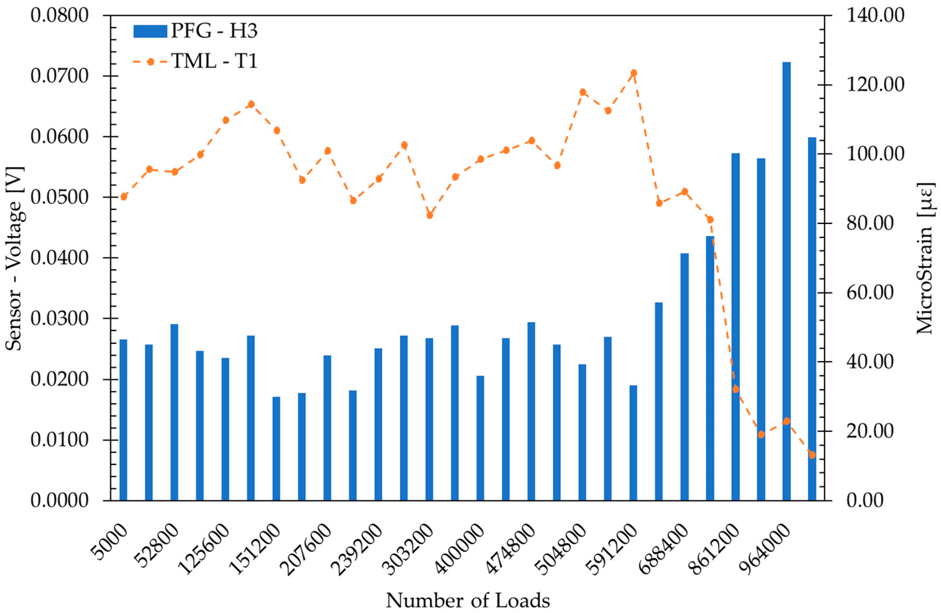
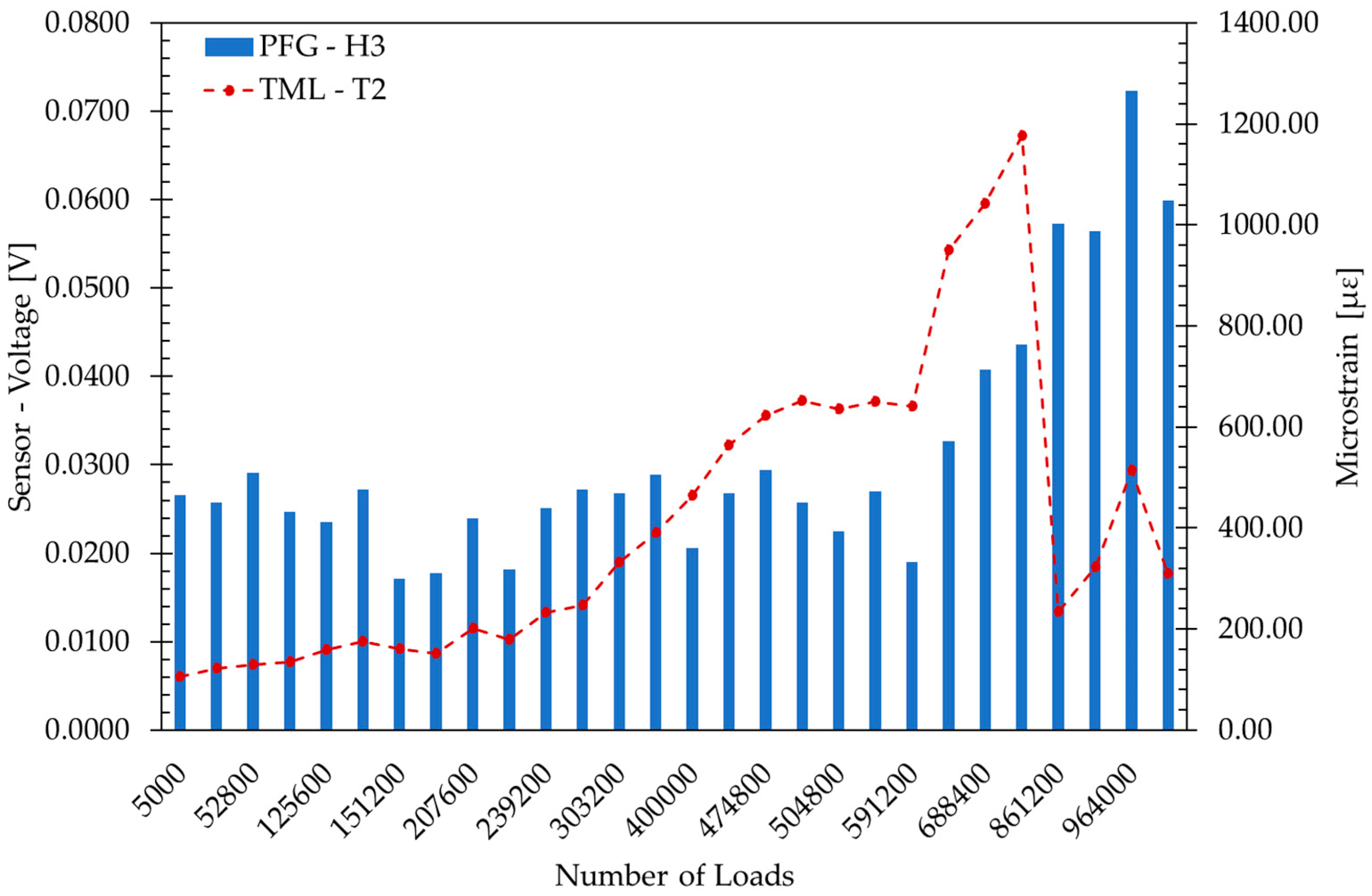
shows the seven thresholds for PFG–H3/H7 and activation number for the “waking-up” of the sensor along with the number of load applications. “Waking-up” of the sensor signifies that it starts recording after a particular number of load applications. Figure 11 (top) shows the CVT for sensor H3, whereas Figure 11 (bottom) shows the CVT for sensor H7.

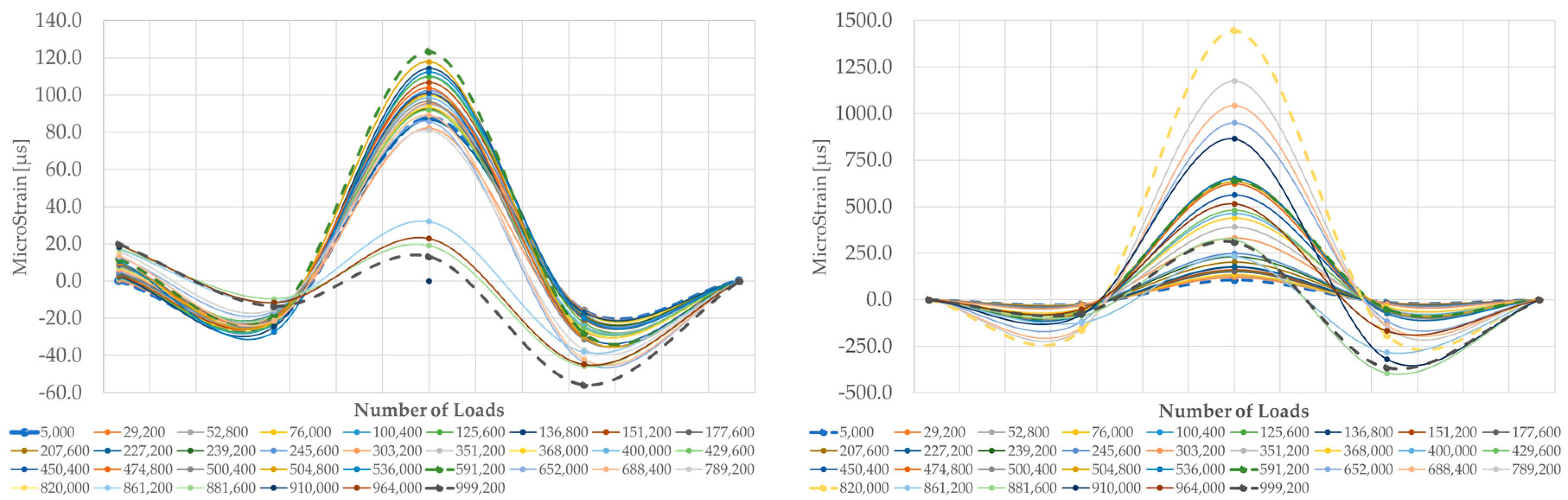
Using Figure 9, Figure 10 and Figure 11, there are specific points that clearly stand out where the change in response, slope, denotes the appearance of damage. Figure 11 (top) supports the previous statement where the “waking-up” of threshold level 3 and onwards occurs. Points located at 125,000, 591,200, and 789,200 load repetitions (3.0, 12.0, and 16.0 years, respectively) were thus selected for developing the maintenance strategies.

At a loading value of 125,000 (equivalent to 3 years of the life cycle), threshold level 2 comes alive. This can be considered as a point where the post-compaction of the AC layer is concluded and damage starts to grow, but at this point, it is also considered as low severity distress. Given that the sensors have indicated that there is something wrong, the routine maintenance that was expected to be carried out at year 8 can be moved up to now take place two years after the sensors have indicated that something is wrong. This intervention is routine maintenance, characterized by minor surface treatments.

The next instance of noted change by the sensors is at an equivalent load of 591,200 (equivalent to 12 years of the life cycle). At this point, the values of threshold levels 1 and 2 have kept growing as expected. The damage is now considered as medium severity, as threshold levels 1 and 2 have changed their slope and threshold levels 3 and 4 are becoming alive as well. Therefore, given this development, another intervention at year 14 can be planned. At year 13 (two years after the trend has now picked up on the sensor/gauge), intervention 1 and 3 can be introduced instead of waiting for year 15, as was planned in the pre-set maintenance plan. Additionally, intervention 2 can be introduced midway between these planned interventions given the fact that the sensor shows the distress is evolving, and this would enable its development to be reduced, prolonging the necessity of corrective maintenance.

At a loading of 789,200 (equivalent to year 16 in the life cycle), the values at threshold levels 1 and 2 grow with no variation in their slope; nonetheless, the values of threshold levels 3 and 4 have increased and threshold levels 5, 6, and 7 have been initiated. This, therefore, infers that the damage is now considered as medium/high severity, indicating that surface cracks are imminent. Therefore, in the optimized plan, interventions can be planned to extend the point at which this will happen. Subsequently, using intervention 3 along with the routine maintenance would be an intervention of less financial impact than that of intervention 4, which is scheduled at year 15 in the baseline.

It is necessary to note here that, while the sensors in the experimental section only provided data for 20 years, these data do allow for a projection of what can happen over a 30-year period, and thus enable the environmental evaluation over this period. This is based on the common interventions over similar times [33], and thus enable the environmental evaluation over this period. As interventions in years 0–20 have been shifted, the subsequent interventions in the following 10 years can then be shifted as well. Therefore, the next intervention to account for is intervention 4 (shown at year 15 in the baseline). In the optimized approach, intervention 1 can be introduced at year 19 (given the inclusion of a thin overlay at year 13), which accounts for routine surface maintenance. This is in line with the visual inspections in the study, showing cracking appearing at a loading of 910,000 (equivalent to year 18). Consequently, major intervention 4 can be performed at year 23, which would then be at a similar stage to that of an intervention in the baseline given the shift of processes.

Finally, at year 30, interventions 1 and 3 can be introduced, which would be at a similar stage to that of an intervention in the baseline, but much less significant than the full intervention 5. This, therefore, indicates that, within the optimized 30-year period under analysis, intervention 5 is not carried out. It must be noted that, over the full life cycle of the pavement, this intervention would be needed. However, by lengthening its life expectancy carrying out more preventative and correction intervention actions, intervention 5 has been shifted out of the assessment period. This means that the impacts, both financially and environmentally, would be spread over a longer period. Considering the loading values and the inferences made from the gate activity, the optimized maintenance plan is given in

Table 4. Optimized maintenance action plans based on responses from piezo floating gate (PFG)-H3 sensors.

Year	0	1	2	3	4	5	6	7	8	9	10	11	12	13	14	15	16	17	18	19	20	21	22	23	24	25	26	27	28	29	30
Optimized Interventions	0	0	0	0	0	1	0	0	0	2	0	0	0	1,3	0	0	0	0	0	1	0	0	0	4	0	0	0	0	0	0	1,3

.

5.2. Optimized Plan Based on Asphalt Strain Gauges Response

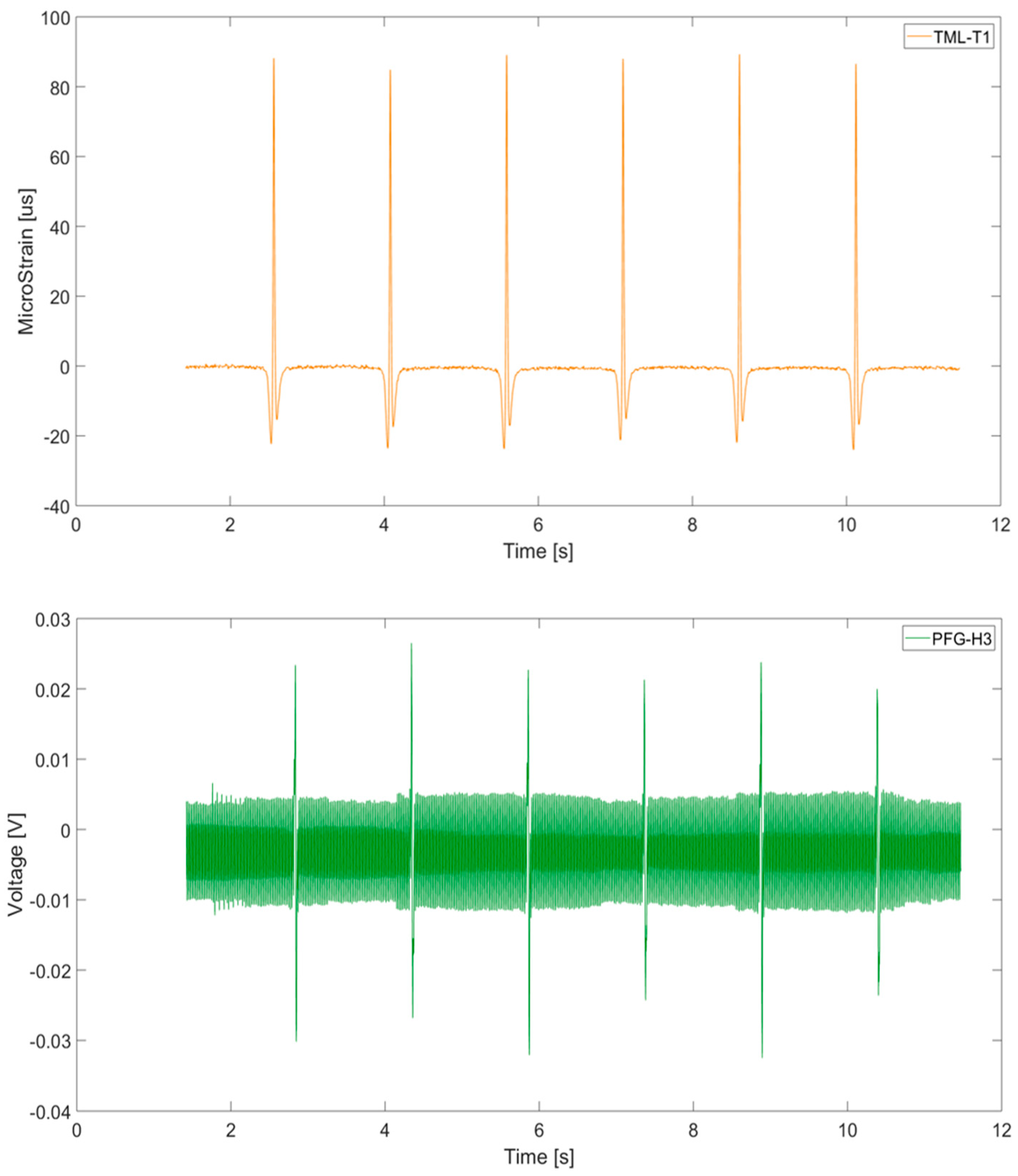
For the strain gauges utilized in the test section, similar trigger points were observed (Figure 9 and Figure 10). Considering the trend shown by sensor T1 (Figure 9), the first point to be considered as a trigger for intervention is at 207,600 loads (equivalent to four years). This point is based on the standard deviation of the max values shown from the sensor, which indicate that there is some damage is occurring within the pavement. The routine maintenance that was expected to be carried out at year 8 can be moved up to two years after the sensors have indicated that something is wrong, similar to the approach taken with the results from the PFG sensors. This is a year after the similar intervention is done with sensor H3. The next instance of noted change by the gauges is at an equivalent load of 591,200 (equivalent to 12 years of the life cycle), which again is similar to the results of sensor H3. However, given that the first noted change from the gauges is a year later than the PFG sensors, it can reasonably be assumed that the damage would have worsened further without any action, as opposed to the road monitoring scenario with the PFG sensor. This assumption is appropriate given the fact that it is the same pavement under analysis. Given this, an additional routine maintenance was inserted to ensure the condition is kept optimal. Therefore, routine maintenance intervention 1 was inserted at year 11 along with intervention 2 at year 10. Intervention 2 can be introduced midway between these planned interventions given the fact that the gauge is showing the distress is evolving, and this would enable its development to be reduced, prolonging the necessity of corrective maintenance. Subsequently, at year 15, intervention 1 and 3 can be introduced at the same point that intervention 4 was planned in the pre-set maintenance plan.

A similar approach, as applied with the plan for the PFG sensors, for the interventions taking place between years 20–30 was also applied for the strain gauge. Therefore, the next intervention to account for is intervention 4 (shown at year 15 in the baseline). In the optimized approach, intervention 1 can be introduced at year 20 (given the inclusion of a thin overlay at year 15), which accounts for routine surface maintenance. This is also in line with the results from the PFG sensors indicating that, at a loading of 900,000 (equivalent to year 18), there are cracks appearing at the surface. Then, subsequent to this, major intervention 4 can be performed at year 24, which would then be at a similar stage to that of an intervention in the baseline given the shift of processes.

Finally, at year 30, interventions 1 and 3 can be introduced, which would be at a similar stage to that of an intervention in the baseline, but much less than the full intervention 5. Considering the loading values and the inferences made from the threshold activity, the optimized maintenance plan is given in

Table 5. Optimized maintenance action plans based on responses from strain gauges.

Year	0	1	2	3	4	5	6	7	8	9	10	11	12	13	14	15	16	17		18	19	20	21	22	23	24	25	26	27	28	29	30
Optimized Interventions	0	0	0	0	0	0	1	0	0	0	2	1	0	0	0	1,3	0	0		0	0	1	0	0	0	4	0	0	0	0	0	1,3

.

Comparable to the optimized plan for the sensors, intervention 5 is not carried out. Additionally, as previously indicated, within the full life cycle of pavement (which would now be more than the 30 years under analysis), this intervention would be needed. Similar to the plan for sensor H3, the impacts, both financially and environmentally, would be allocated over a longer period, making the effect less per year.

6. The Use of Life Cycle Assessment

Having identified different maintenance pipelines for each scenario, it was noted that, using the monitoring techniques, there are now more interventions occurring. They are of a lesser value in terms of work and financial costs, but together they signify a larger number of interventions than in the pre-planned system. Therefore, the question arises as to whether using more interventions will cause more damage to the environment, even if they are extending the life of the pavement. Given the knowledge that the maintenance and rehabilitation of asphalt pavements can be quite environmentally impactful [35], the next step was to quantify their environmental impacts in terms of LCA indicators.

6.1. Goal and Scope Definition

The study was performed in order for the environmental impacts of the three alternative product systems to be quantified and compared. The product systems include the maintenance phase of the same stretch of asphalt pavement. In the baseline scenario, the maintenance regime to be followed is one typical of usually implemented typical predefined maintenance strategies. The two alternatives consist of optimized maintenance planning based upon the data acquired from the different types of sensing technologies that have been embedded in the corresponding pavement structures. The study thus aims to quantify the environmental burdens affiliated with the maintenance pipeline of the two optimized scenarios and identify whether they exhibit an improvement compared with the baseline.

6.2. Functional Unit

The functional unit that was utilized for the specific study can be described as 1 m² of the asphalt pavement’s surface, along with the underlying asphaltic layers, providing adequate performance for a period of 30 years. In detail, two bituminous layers are technically included and are both composed by the EME2 asphalt mixture, a high modulus mixture widely used in road engineering in France [36]. The functional unit can be seen in Figure 12.

6.3. System Boundaries

Having defined the functional unit, the next step was the definition of the system boundaries. As defined in different guidance documents [22,23,37], the four stages of an asphalt pavement’s life cycle are the product stage, the construction stage, the use stage, and the end of life stage. In this study, the selected system boundaries are limited to the use stage and specifically to B2: maintenance, B3: repair, and B4: replacement. The reason behind this methodological choice is the fact that the LCA exercises are conducted for the same pavement structure and the same analysis period of 30 years. Thus, the environmental impacts arising from the product, the construction, and the end of life stages would be the same. However, having optimized maintenance pipelines per alternative also indicates that there are potential differences in their environmental severity. The system boundaries for all three alternatives can be seen in Figure 13. However, it is worth mentioning that, in the use phase (i.e., maintenance, repair, replacement), the processes related to the raw materials needed to be extracted in order for the maintenance to be achieved; their transport to the mixing plant and the construction site, along with the production of products necessary for the maintenance of the pavements, were included in the system boundaries. It should also be noted that more frequent interventions in the road segment, even if of lower significance/duration), could potentially impose higher costs for the users. However, as the analysis conducted in this study focuses only on the environmental pillar of sustainability, the user/agency costs were not taken into consideration. Moreover, the required interventions now, in the optimized scenario, consist of mainly surface treatments and not structural interventions. That would mean that, indeed, a higher amount of interventions would occur, but at the same time, these interventions would cost, in terms of time, significantly less. Finally, the environmental impacts of these interventions have already been quantified, utilizing the maintenance itself as system boundaries. Environmental impacts related to traffic congestion or rerouting were not taken into consideration, based on the very definition of our product system.

For the completion of the LCA case studies, Gabi ts, by Thinkstep [38], was utilized along with the Gabi Professional and Ecoinvent 3 databases. Moreover, no primary data were acquired, and instead reputable data sources and literature, reports, international standards, product category rules (PCRs), and environmental product declarations (EPDs) were used [22,23,37,39,40,41,42,43]. In terms of impact assessment methodology, ReCiPe 2016, Hierarchist (H) [44] was utilized for both Mid and Endpoint indicators.

6.4. Life Cycle Assessment Results

As mentioned before, ReCiPe 2016 (H) was utilized as the impact assessment methodology in this study. Thus, as proposed within the very same methodology and for reasons concerning the increased accuracy of the study, the analysis of the LCA impact category indicators was conducted in two levels: MidPoint and EndPoint. The midpoint indicators are associated with a wider range of analysis, while the endpoint impact category indicators correspond to three aggregated indicators, also characterized as areas of protection (AOP). It is recommended for the two levels of analyses to be implemented in parallel, in order for more informed results to be acquired [44].

6.4.1. MidPoint Impact Category Indicators

Following the life cycle impact assessment and life cycle interpretation phases that were undertaken for the realization of this study, the MidPoint impact category indicators can be found in Figure 14 for all three scenarios. This radar graph indicates the relative percentage variation of the values of the MidPoint impact category indicators compared with the baseline. The latter is depicted as the black dashed line, while in red and green colors, the scenarios with the strain gauges and the PFG sensors can be found, respectively.

From Figure 14, it can be seen that, in both the scenarios, where embedded sensing technologies were utilized, all the MidPoint impact category indicators exhibit lower values compared with the baseline. This can be explained by the fact that, when the aforementioned sensing technologies are utilized, the amount of available data about the condition of the pavement is significantly higher compared with situations where no sensors are utilized. Thus, more informed decisions regarding the way of selecting the most appropriate maintenance strategy and the most beneficial time interval to execute it can be achieved. Moreover, it can also be said that, when PFG sensors are used, the values of the MidPoint indicators are slightly lower compared with the two other scenarios, because, with this technology, it became possible to acquire “warning data” concerning the condition of the pavement earlier that when conventional strain gauges were utilized.

6.4.2. EndPoint Impact Category Indicators

The next step to be undertaken according to the ReCiPe 2016 (H) impact assessment methodology is the quantification of the EndPoint impact category indicators. They are able to provide a broader view of the impacts that the studied scenarios impose in the environment. In detail, they allocate the damages originating from the maintenance regimes of the three scenarios in three areas of protection; namely, damage to human health measured in disability-adjusted life years (DALY), damage to ecosystems expressed as time-integrated species loss, and damage to resource availability with surplus cost as its metric. In Figure 15, the values of the EndPoint impact category indicators per scenario are displayed.

As Figure 15 depicts, the values of the Endpoint indicators are slightly reduced for both scenarios that utilize embedded sensing technologies. In detail, the values of the EndPoint indicators for the scenario with the PFG sensors are slightly reduced compared with those corresponding to the scenario where conventional strain gauges were used.

7. Summary and Conclusions

In this study, two embedded sensing technologies (PFG sensors and conventional asphalt strain gauges) were used to develop optimized maintenance plans for road pavement management. In addition, in order to assess the environmental impact of the optimized approaches, a life cycle assessment (LCA) exercise was carried out.

The sensors were located at the bottom of the asphalt layer of a section of the APT facility owned and managed by the IFSTTAR. Their responses were collected over the duration of the experiment (three months) and analyzed in terms of maximum strain/voltage evolution with the increasing number of loads. The results show that both technologies depict the weakening of the pavement structure with strain and voltage measurements having a good correlation for the majority of the experiment. It was, however, noted that there were significant differences in the maximum microstrain measurements from the strain gauges for the T1 and T2 gauges. This is important as it demonstrates that, for this technology, it is critical to have an array of devices employed to allow for critical evaluation and accuracy by pavement engineers. This issue was not detected with the results of the PFG sensors, as there was more consistency in the results of these sensors, and thus this represents an advantage of utilizing this technology. Additionally, the newer version of piezoelectric sensors is wireless, which decreases field installation complexity and creates more flexible data transmission protocols that can be associated with the strain gauges. Furthermore, piezoelectric sensors will be categorized as low-cost solutions, which makes them more attractive not only for research projects, but for real case studies.

Sensors T2 and H3 (Figure 10) suffer a drastic change in slope at approximately 600,000 load repetitions. After this point, defined as critical, damage in the AC layer will grow at a much higher rate, which may lead to structural failure if no maintenance is scheduled. The results from sensor H3, Figure 11 (top), support this as the middle thresholds (3 and 4, Table 3) also become alive at approximately 600,000 load repetitions. Finally, surface cracking is seen around 900,000 load repetitions, when all the thresholds have been wakened up, which validates the idea of using PFG sensors for preventive pavement monitoring.

While the sensor results allowed for the generation of optimized pavement maintenance strategies, the LCA case study allowed for an evaluation of the environmental friendliness of these actions. The evaluation was done utilizing a commercial software, Gabi ts, and for life cycle impact assessment methodology, ReCiPe 2016 (H) was selected. Through this assessment, it was shown that both strategies presented environmental benefits during the maintenance phase of the asphalt pavements, with the PFG sensors providing the greater benefits of the two. It can thus be deduced that, when sensing technologies are embedded in the pavement structure and are able to provide the decision-makers with “in-time” information about the condition of the pavement, more informed choices can be made that lead to more environmentally friendly maintenance regimes, compared with the case when sensors are absent. A critical point in the analysis is that the optimized schedules allow for an extended life cycle of the pavement. This is done by carrying out more preventative maintenance interventions and not waiting on the more environmentally harmful corrective maintenance interventions when pavement failure has already occurred.

These results present a pipeline for practical application of utilizing the embedded technologies within the pavement management industry. The use of the sensors has practical advantages given their embedded nature and, therefore, the lack of intrusiveness provided by the data collected from these sensors as compared with other technologies that require consistent physical intervening surveys. However, there is still more research to be done on these technologies given doubts with regards to the technologies’ life expectancy, the reliability of the results, and their end of life strategies. The failure of sensors needs to be further examined in future work as well, because once a sensor has suffered failure, there is no easy solution given that they are embedded. Given these drawbacks to the technologies, this study helps to bridge these gaps by providing an understanding how to utilize the data from these sensors and how they can be interpreted for maintenance strategy formulation. It should also be noted that the cost of implementation of the sensors needs to be fully understood in future works, as this is a key component to practical implementation. More real-world experiments, similar to those in the study, will help validate and support the use of these technologies moving forward. Future developments should line up with the miniaturization of the technology, reducing complexity for field deployments, and providing easy ways for visualization and management of the data.

References

1. Vandam, T.J.; Harvey, J.T.; Muench, S.T.; Smith, K.D.; Snyder, M.B.; Al-Qadi, I.L.; Ozer, H.; Meijer, J.; Ram, P.V.; Roesier, J.R.; et al. Towards Sustainable Pavement Systems: A Reference Document FHWA-HIF-15-002; Federal Highway Administration: Washington, DC, USA, 2015. [Google Scholar]
2. International Road Federation (IRF). IRF World Road Statistics 2018 (Data 2011–2016); International Road Federation (IRF): Brussels, Belgium, 2018. [Google Scholar]
3. Peterson, D. National Cooperative Highway Research Program Synthesis of Highway Practice Pavement Management Practices. No. 135; Transportation Research Board: Washington, DC, USA, 1987; ISBN 0309044197. [Google Scholar]
4. Li, X.; Goldberg, D.W. Toward a mobile crowdsensing system for road surface assessment. Comput. Environ. Urban Syst. 2018, 69, 51–62. [Google Scholar] [CrossRef]
5. Radopoulou, S.C.; Brilakis, I. Improving Road Asset Condition Monitoring. Transp. Res. Procedia 2016, 14, 3004–3012. [Google Scholar] [CrossRef] [Green Version]
6. Ragnoli, A.; De Blasiis, M.; Di Benedetto, A. Pavement Distress Detection Methods: A Review. Infrastructures 2018, 3, 58. [Google Scholar] [CrossRef] [Green Version]
7. Coenen, T.B.J.; Golroo, A. A review on automated pavement distress detection methods. Cogent Eng. 2017, 4, 1374822. [Google Scholar] [CrossRef]
8. Inzerillo, L.; Di Mino, G.; Roberts, R. Image-based 3D reconstruction using traditional and UAV datasets for analysis of road pavement distress. Autom. Constr. 2018, 96, 457–469. [Google Scholar] [CrossRef]
9. Xue, W.; Wang, D.; Wang, L. A review and perspective about pavement monitoring. Int. J. Pavement Res. Technol. 2012, 5, 295–302. [Google Scholar]
10. Lajnef, N.; Rhimi, M.; Chatti, K.; Mhamdi, L.; Faridazar, F. Toward an integrated smart sensing system and data interpretation techniques for pavement fatigue monitoring. Comput. Civ. Infrastruct. Eng. 2011, 26, 513–523. [Google Scholar] [CrossRef]
11. Merenda, M.; Praticò, F.G.; Fedele, R.; Carotenuto, R.; Corte, F.G. Della A real-time decision platform for the management of structures and infrastructures. Electronics 2019, 8, 1180. [Google Scholar] [CrossRef] [Green Version]
12. Fedele, R.; Praticò, F.G.; Carotenuto, R.; Della Corte, F.G. Energy savings in transportation: Setting up an innovative SHM method. Math. Model. Eng. Probl. 2018, 5, 323–330. [Google Scholar] [CrossRef]
13. Hasni, H.; Alavi, A.H.; Chatti, K.; Lajnef, N. A self-powered surface sensing approach for detection of bottom-up cracking in asphalt concrete pavements: Theoretical/numerical modeling. Constr. Build. Mater. 2017, 144, 728–746. [Google Scholar] [CrossRef]
14. American Association of State Highway and Transportation Officials (AASHTO). Pavement Management Guide; American Association of State Highway and Transportation Officials (AASHTO): Washington, DC, USA, 2012. [Google Scholar]
15. Xue, W.; Wang, L.; Wang, D.; Druta, C. Pavement Health Monitoring System Based on an Embedded Sensing Network. J. Mater. Civ. Eng. 2014, 26, 04014072. [Google Scholar] [CrossRef]
16. Duong, N.S.; Blanc, J.; Hornych, P.; Bouveret, B.; Carroget, J.; Le feuvre, Y. Continuous strain monitoring of an instrumented pavement section. Int. J. Pavement Eng. 2018, 8436, 1435–1450. [Google Scholar] [CrossRef]
17. Gaborit, P.; Sauzéat, C.; Di Benedetto, H.; Pouget, S.; Olard, F.; Claude, A.; Monnet, A.J.; Audin, R.M.; Sauzéat, C.; Di Benedetto, H.; et al. Investigation of highway pavements using in-situ strain sensors. Int. Conf. Transp. Infrastruct. 2013, 28, 331. [Google Scholar]
18. Blanc, J.; Hornych, P.; Duong, N.S.; Blanchard, J.Y.; Nicollet, P. Monitoring of an experimental motorway section. Road Mater. Pavement Des. 2017, 20, 74–89. [Google Scholar] [CrossRef]
19. Stripple, H. Life Cycle Assessment of Road, A Pilot Study for Inventory Analysis; IVL RAPPORT. 1210; IVL: Linköping, Sweden, 2001; Volume 2. [Google Scholar]
20. Carlson, A. Life Cycle Assessment of Roads and Pavements—Studies Made in Europe; VTI Rapp. 736A; Statens väg-och transportforskningsinstitut: Linköping, Sweden, 2011; Volume 22. [Google Scholar]
21. ECRPD. Energy Conservation in Road Pavement Design, Maintenance and Utilisation. 2010, pp. 1–63. Available online: https://ec.europa.eu/energy/intelligent/projects/sites/iee-projects/files/projects/documents/ecrpd_publishable_report_en.pdf (accessed on 29 December 2019).
22. The International Standards Organisation. Environmental Management—Life Cycle Assessment—Requirements and Guidelines; ISO 14044; The International Standards Organisation: Geneva, Switzerland, 2006; pp. 652–668. [Google Scholar]
23. International Organization for Standardization. ISO 14040-Environmental Management—Life Cycle Assessment—Principles and Framework; The International Standards Organisation: Geneva, Switzerland, 2006; Volume 3, p. 20. [Google Scholar]
24. Chappat, M.; Bilal, J. La route écologique du futur—Analyse du Cycle de Vie, Consommation d’énergie & émission de gaz à effet de serre. Développement Durable 2003, 40. [Google Scholar]
25. Häkkinen, T.; Mäkelä, K. Environmental Impact of Concrete and Asphalt Pavements; Technical Research Center of Finland: Espoo, Finland, 1996; ISBN 9513849074. [Google Scholar]
26. Mroueh, U.M.; Laine-Ylijoki, J.; Eskola, P. Life-cycle impacts of the use of industrial by-products in road and earth construction. Waste Manag. Ser. 2000, 1, 438–448. [Google Scholar]
27. Hoang, T.; Jullien, A.; Ventura, A.; Crozet, Y. A global methodology for sustainable road—Application to the environmental assessment of French highway. In Proceedings of the 10 DBMC International Conference On Durability of Building Materials and Components, Lyon, France, 17–20 April 2005. [Google Scholar]
28. Tokyo Measuring Instruments Lab. TML Pam E-2020C Tranducers 2017. Available online: https://tml.jp/eng/documents/Catalog/Transducers_E2020C.pdf (accessed on 12 November 2019).
29. Karim, C.; Alavi, A..; Hassene, H.; Lajnef, N.; Faridazar, F. Damage Detection in Pavement Structures Using Self-powered Sensors. In Proceedings of the 8th RILEM International Conference on Mechanisms of Cracking and Debonding in Pavements, Nantes, France, 6–9 June 2016; Springer: Berlin, Germany, 2016; pp. 665–671. [Google Scholar]
30. Lajnef, N.; Chatti, K.; Chakrabartty, S.; Rhimi, M.; Sarkar, P. Smart Pavement Monitoring System; Federal Highway Administration: Washington, DC, USA, 2013. [Google Scholar]
31. Alavi, A.H.; Hasni, H.; Lajnef, N.; Chatti, K.; Faridazar, F. An intelligent structural damage detection approach based on self-powered wireless sensor data. Autom. Constr. 2016, 62, 24–44. [Google Scholar] [CrossRef]
32. Loboratoire Central des Ponts et Chaussées. French Design Manual for Pavement Structures; Loboratoire Central des Ponts et Chaussées: Paris, France, 1997. [Google Scholar]
33. SETRA-LCPC. Catalogue des Structures Types de chaussées Neuves; SETRA-LCPC: Paris, France, 1998. [Google Scholar]
34. Laurent, G. Evaluation économique des chaussées en béton et classiques sur le réseau routier national français; ETUDES ET RECHERCHES DES LABORATOIRES DES PONTS ET CHAUSSEES-SERIE: ROUTES CR 33; ETUDES ET RECHERCHES DES LABORATOIRES DES PONTS ET CHAUSSEES: Paris, France, 2004. [Google Scholar]
35. Mantalovas, K.; Di Mino, G. The sustainability of reclaimed asphalt as a resource for road pavement management through a circular economic model. Sustainbility 2019, 11, 2234. [Google Scholar] [CrossRef] [Green Version]
36. Petho, L.; Denneman, E. Implementing EME2, the French high modulus asphalt in Australia. In Proceedings of the 6th Eurasphalt & Eurobitume Congress, Prague, Czech Republic, 1–3 June 2016. [Google Scholar]
37. EAPA. Guidance Document for Preparing Product Category Rules (Pcr) and Environmental Product Declarations (Epd) for Asphalt Mixtures; EAPA: Arlington County, VA, USA, 2017; p. 43. [Google Scholar]
38. Thinkstep AG Gabi ts 2019. Available online: https://www.thinkstep.com/content/gabi-databases-2019-edition (accessed on 29 December 2019).
39. The Norwegian EPD Foundation. Product-Category Rules (PCR) for Preparing an Environmental Product Declaration (EPD) for Product Group Asphalt and Crushed Stone; The Norwegian EPD Foundation: Skien, Norway, 2009. [Google Scholar]
40. EAPA. The Use of Warm Mix Asphalt; EAPA—Position paper; EAPA: Arlington County, VA, USA, 2014; p. 23. [Google Scholar]
41. BRE. Product Category Rules for Type III Environmental Product Declaration of Construction Products to EN 15804:2012; BRE Group: Watford, UK, 2013; p. 43. [Google Scholar]
42. European Bitumen Association. Life Cycle Inventory: Bitumen; European Bitumen Association: Harrogate, UK, 2012; ISBN 2930160268. [Google Scholar]
43. EC-European Commission. COMMISSION RECOMMENDATION of 9 April 2013 on the Use of Common Methods to Measure and Communicate the Life Cycle Environmental Performance; EC-European Commission: Brussels, Belgium, 2013; pp. 1–45. [Google Scholar]
44. Huijbregts, M.A.J.; Steinmann, Z.J.N.; Elshout, P.M.F.; Stam, G.; Verones, F.; Vieira, M.D.M.; Zijp, M.; van Zelm, R. ReCiPe 2016: A harmonized life cycle impact assessment method at midpoint and enpoint level—Report 1: Characterization. Natl. Inst. Public Health Environ. 2017, 22, 138–147. [Google Scholar]
Figure 1. Typical uses of pavement management information in a pavement management system (PMS).
Infrastructures 05 00004 g001
Figure 2. Tokyo Measuring Instruments Lab (TML) strain gauge.
Infrastructures 05 00004 g002
Figure 3. Piezo floating gate (PFG) sensor composition. PVDF, polyvinylidene fluoride.
Infrastructures 05 00004 g003
Figure 4. Distribution of sensors within the pavement structure.
Infrastructures 05 00004 g004
Figure 5. Structure of pavement used in the test section.
Infrastructures 05 00004 g005
Figure 6. Measurement from sensors T1 (TML) (top) and sensors H3 (PFG) (bottom), after 5000 loads.
Infrastructures 05 00004 g006
Figure 7. Average gauge signal for TML–T1 and TML–T2, respectively, with characteristic points.
Infrastructures 05 00004 g007
Figure 8. Evolution of voltage for PFG–H3 and PFG–H5, respectively.
Infrastructures 05 00004 g008
Figure 9. Sensors T1 and H3 measurements evolution.
Infrastructures 05 00004 g009
Figure 10. Sensors T2 and H3 measurements evolution.
Infrastructures 05 00004 g010
Figure 11. Cumulative voltage time (CVT) for sensor H3 and H7, respectively.
Infrastructures 05 00004 g011
Figure 12. Functional unit of the life cycle assessment (LCA) exercises.
Infrastructures 05 00004 g012
Figure 13. System boundaries of the product system.
Infrastructures 05 00004 g013
Figure 14. Relative percentage variation of the MidPoint indicators’ values.
Infrastructures 05 00004 g014
Figure 15. Values of the EndPoint impact category indicators per scenario.
Infrastructures 05 00004 g015