1. Introduction
Infrastructure networks are composed of many different assets that work together to provide service, e.g., the transportation of goods and people at specified speeds with specified levels of safety [
1,
2,
3,
4]. These assets are managed over time to ensure they continue to provide the required service, which includes the determination of the interventions to execute within an upcoming planning period, i.e., maintenance, renewal, improvements and extensions interventions, taking into consideration the goals of the infrastructure manager, intervention strategies and the state of the assets [
5]. The balancing of the costs of possible interventions with their ability to ensure that this service is provided requires consideration of each of the individual assets and how they work together in the network [
6,
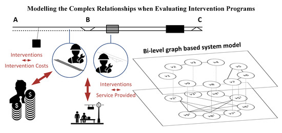
7]. On the asset level, this includes consideration of the intervention costs due to labour, material, the use of machinery, planning, etc. On the network level, this includes consideration of how interventions lead to interruptions in service.
When determining intervention programs, a relatively sophisticated system model is required that describes and models the complex and nonlinear relationship between the candidate interventions, the interventions costs and the service provided by infrastructure networks. The candidate interventions refer thereby to all interventions that could be included in the intervention program, and about which infrastructure managers have to make decisions. For simplification, they are referred to simply as interventions in the remaining of the paper. A sophisticated system model is required because the costs and interruptions to service cannot simply be estimated per intervention and summed [
8,
9]. The system model needs to describe and model the relationships consistently in different situations. The system model is not to be confused with an optimisation model. It mathematically describes the relationships of the interventions and the costs of an intervention program. Optimisation models describe the decision problem of determining the optimal intervention program using some kind of system model to describe the relationships between the impacts of decisions.
The relationships between interventions, intervention costs and the service provided are based on economical, topological, structural and resource dependencies [
10,
11,
12,
13,
14]. Economical dependencies refer to situations where the cost of multiple interventions differs from the sum of the cost for individual interventions [
11,
12]. Topological dependencies refer to situations where the functionality of the network is affected by the spatial location of the investigated assets [
10,
14], which describe a nonlinear relationship between the individual interventions and the service provided. Structural dependencies refer to situations where an intervention on one asset either implies or prohibits an intervention on another asset [
14], which define interventions whose execution needs to be in series. Resource dependencies refer to situations where interventions on assets share a common resource [
13]. They ether limit the overall selection of interventions in an intervention program, i.e., available budget, or prohibit two interventions to be executed at the same time, i.e., due to the use of the same work team or machinery.
In the past, researchers have used a variety of system models that make different trade-offs between the consideration of the complex relationships and the simplicity in their modelling in order to enable the formulation of optimisation models that can be solved without heuristics. These models have included those using linear combination [
15,
16,
17,
18,
19], group state [
20,
21,
22,
23,
24], graph theory [
25,
26,
27], reliability block diagrams [
28,
29,
30,
31,
32,
33,
34,
35,
36,
37,
38,
39,
40,
41] and detailed simulations in bi-level models [
42,
43,
44,
45,
46,
47]. Existing system models using linear combination, group state and graph theory all enable building optimisation models using integer linear programs that can be solved by global optimisation techniques, but their accuracy of the model of the relationship between interventions, interventions costs and the service provided by infrastructure networks could be improved. System models using linear combination estimate the costs and the effect on service as the sum of the costs of all selected alternatives. Economical and topological dependencies are only considered within, but not across, the defined alternatives [
16,
17,
19], which requires to define additional alternative for each additional dependency. Group state system models consider economical or topological dependencies by counting the common shared costs or the shared effect on service between interventions only once per group [
20,
21]. They are limited in respect of modelling overlapping and mutually influencing relationships between multiple groups of interventions due to the combination of economical, topological and structural dependencies. The existing graph theory system models only consider binary pairwise relationships between interventions, which requires simplifications in the consideration of relationships between multiple interventions, i.e., in estimating the effect on service. Reliability block diagram and bi-level system models are generally able to model the network state based on the assets state, i.e., the relationship between interventions and the effect on service. They use, therefore, more complex and non-linear mathematical formulations, which lead to optimisation models requiring heuristic algorithms. System models using reliability block diagram describe the effect on service by a combination of summation and multiplications of the selection of interventions [
8,
37]. This enables to estimate properly the network state at a given point in time considering topological dependencies, but limits the consideration of the differences in the intervention duration and in modelling multiple network states over time, which is required when estimating the effect on service associated with an intervention program. Bi-level system models model the intervention selection and the intervention costs in an asset level model and the effect on service in a separate model on the network level, i.e., detailed traffic simulations. This enables detailed modelling of the relationships and estimation of the intervention costs and the effect on service associated with an intervention program, but requires heuristics to optimise the nested optimisation models.
Contrary to the above mentioned system models, the type of system models proposed in this paper (1) are suitable for the estimation of the intervention costs and the effects on service associated with an intervention program, (2) do not neglect or overly simplify the relationships between interventions, interventions costs and the service provided by infrastructure networks, and (3) enable the construction of optimisation models using mixed integer linear programs that can find the optimal sets of interventions without the help of heuristics. The type of system model proposed allows explicit modelling of the specific interventions and the intervention costs on the asset level, and the effects on service on the network level. It also enables accurate modelling of intervention costs as a function of the spatial and temporal distribution of the interventions, referred to herein as economic dependencies, and the impact on the service provided as a function of the topology of the networks, referred to herein as topological dependencies. It enables the formulation of mixed integer linear programs that can be solved to find the global optimum without the help of heuristics.
The type of system model proposed in this paper uses graph theory, which enables the modelling of many different kind of relationships in system model [
48,
49,
50]. In order to improve the modelling of the relationships between the interventions, the intervention costs and the service provided from that done in past graph theory models, a bi-level graph model is developed. The asset level models the interventions on the assets as nodes and their economical dependencies as edges. The network level models the duration of the network states that must exist to enable the execution of the interventions of the intervention program, considering the possible interventions on the assets and the topological dependencies between them. The layers represent the possible network states and contain nodes representing the interventions that are possible to be executed with the particular network state, and edges representing the requirement of sequential execution of interventions, i.e., interventions that are not possible to be executed at the same time. The service disturbance-oriented categorisations of the interventions on infrastructure networks and the hierarchical network state structure enable this type of system model to be used for infrastructure networks comprised of assets of different types, e.g., track, bridges, tunnels and power supply systems, upon which interventions of different types, e.g., maintenance, renewal, improvement and extension, can be executed. An example can be found in [
10], where an optimisation model based on this type of system model was used successfully to determine the optimal intervention programs for a railway network.
The remainder of the paper consists of the list of notations used in the paper in
Section 2.
Section 3 describes the proposed type of system model.
Section 4 describes the algorithm to construct system models of this type using a fictive railway network consisting of the railway track, switches, bridges, tunnels and the overhead power supply.
Section 5 discusses the construction of optimisation models enabling the determination of optimal intervention programs using the proposed system model.
Section 6 and
Section 7 contain the discussion and conclusions of the work.
3. A New Bi-Level Graph Theory System Model
The bi-level graph theory system model proposed here combines the advantages of the bi-level impact system models, which enable the required modelling of economical dependencies on the asset level and the topological dependencies on the network level, with the advantages of graph theory system models, which enable the formulation of optimisation models that can find optimal solutions without the reverting to heuristics. The new model overcomes the limitation of existing graph theory models by modelling the relationship between interventions and the service provided explicitly on the network level. Thus, the system model proposed is capable of modelling the relationships between the interventions, the intervention costs and the service in a way that includes the economical and topological dependencies so that their effect on the intervention costs and impact on the service can be accurately considered.
It models the intervention costs and the impacts on the service provided together as total costs
that occur on two levels, i.e., the asset level (
) and the network level (
) (Equation (1)). The asset level models the interventions and the economical dependencies between them considering the relationships between the interventions and the intervention costs. The network level models the duration of the network states that must exist to enable one or more interventions to be executed. It is at this level that the intervention costs related to work zones and the impacts on the service provided are modelled.
The system model is described by graph
(
Figure 1). It consists of the asset level subgraph
, the network level subgraph
and the inter-level edges
, where an edge
connects the node
of the asset level with node
in network state
. The following sections describe the system model and how the dependencies between interventions are modelled on the asset and network level in order to enable the estimation of the asset and network level intervention costs and disruptions to service for an intervention program.
3.1. Asset Level
Intervention costs, including the costs of material, labour, planning and logistics are modelled at the asset level. This includes the consideration of economical dependencies that affect intervention costs, e.g., shared set-up costs of the interventions. They imply that the total costs on the asset level are not equal to the sum of the individual costs.
The asset level model is graph
with the set of nodes
and the set of edges
(upper part in
Figure 1). Each node
represents an intervention
. Each undirected edge
represents an economical dependency between
and
. In
Figure 1, the concept of the asset level is illustrated with interventions 1 to 9 represented by nodes
v1 to
v9, and their economical dependencies. For example,
v3 is economical dependant to
v2 and
v4.
The total costs on the asset level
are equal to the sum of the variable intervention costs
and the shared costs
of each connected component of graph
(Equation (2)). In
Figure 1, the connected components are (
v2,
v3,
v4) and (
v5,
v6,
v7). Whether the costs of an intervention is to be considered or not depends on the selection of the intervention in the intervention program indicated by the binary variable
that is 1 if the intervention represented by node
is selected. The shared costs of economical dependent interventions
are considered when at least one node of the connected component is selected, which is expressed by binary variable
.
3.2. Network Level
The disruptions to service, e.g., costs due to longer travel time for network users are modelled on the network level. These costs are affected by topological dependencies between interventions, which implies that the total costs on the network level are not equal to the sum of the individual costs.
Instead of considering the disturbance of each intervention separately, the network level costs are quantified by considering to which extent and for how long service is disturbed by the execution of the interventions. Since the interventions of an intervention program are not all executed at the same time, but scheduled within the planning period, the extent of the service disruption varies throughout the planning period [
51]. Network states
are used to model this variation, e.g., a shutdown of one of two parallel lines, a shutdown of two parallel lines. The total service disruption costs
are the sum of the durations of all network states
required for the implementation of the intervention program, i.e., the execution of the interventions, multiplied by their costs
(Equation (3)).
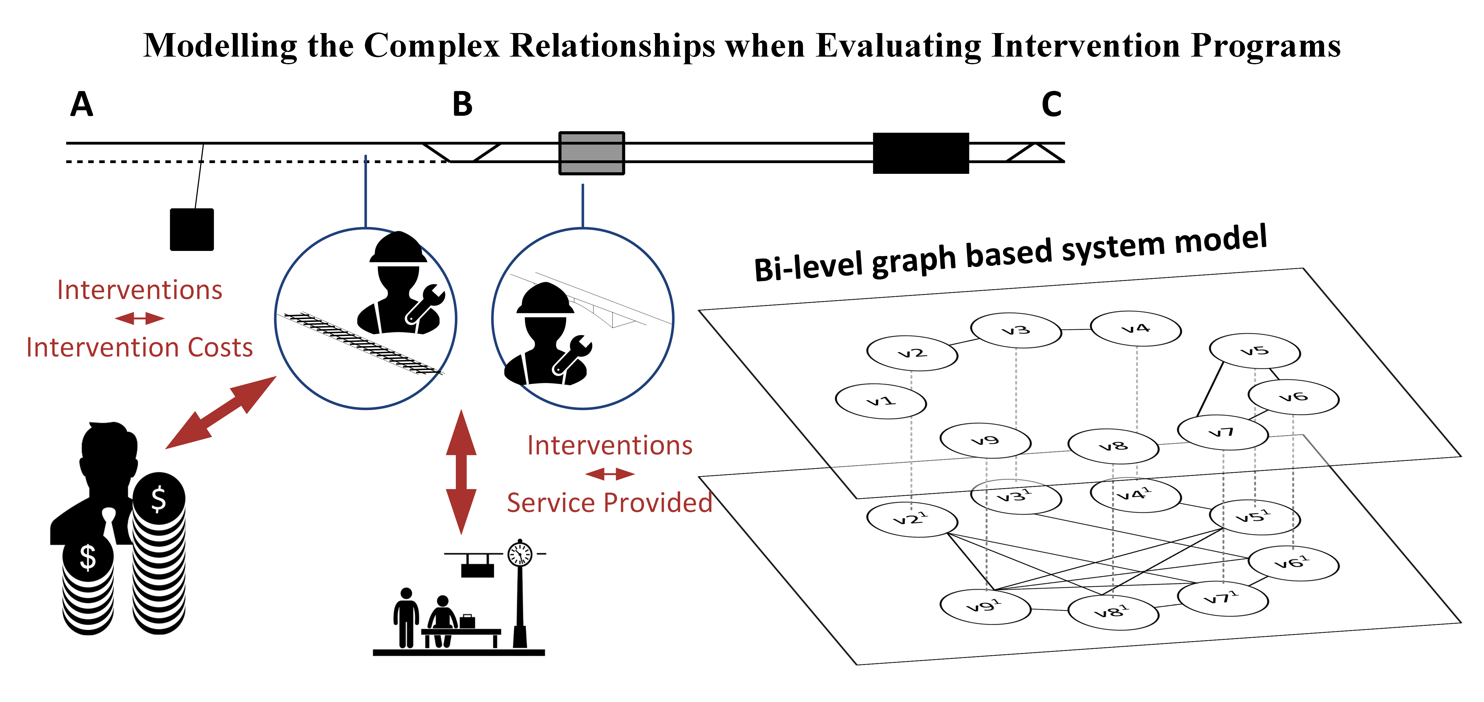
The network level has to model the topological dependencies between the interventions in respect to the network state durations required to implement the intervention program. This is modelled by considering layers in subgraph . Each layer represents a network state. A node represents the execution of an intervention with network state . An edge represents the possibility for parallel execution of and with network state .
The illustration in
Figure 1 considers three different network states. Each state only considers the interventions that could be executed in this state. The edges represent interventions that can be executed in parallel. For example,
v3,
v4,
v7 and
v8 can be executed with network state 2.
v7 and
v8 can be executed parallel in time. The intervention represented by
v1 does not disturb the service and is therefore not considered in any network state, which represent different disruptions on the service provided.
Each node
is assigned with the duration of the intervention that is represented by node
with network state
, i.e.,
. The decision whether an intervention is executed with network state
or not is considered by variable
. The duration required of network state
, i.e.,
, equals to the maximal duration of non-parallel interventions. This means that the durations of interventions executed in parallel with other interventions can be subtracted. Therefore, each edge
is assigned with the duration the execution of the intervention of node
is in parallel to the execution of the intervention of node
, i.e.,
. Additionally, each node is assigned with a relevant duration
equalling the intervention duration that is not parallel to another interventions (Equation (4)). The total duration network state
is required, is equal to the sum of the relevant durations assigned to all nodes (Equation (5)). The durations of parallel executions
are subject to the constraint that they cannot be larger than the relevant duration assigned to node
(Equation (6)). The sum in Equation (6) considers that different interventions may be execute in parallel to the intervention of node
that belong to the same connected component
in the asset level, and require therefore to be executed in series to themselves.
4. Algorithm to Build the System Model
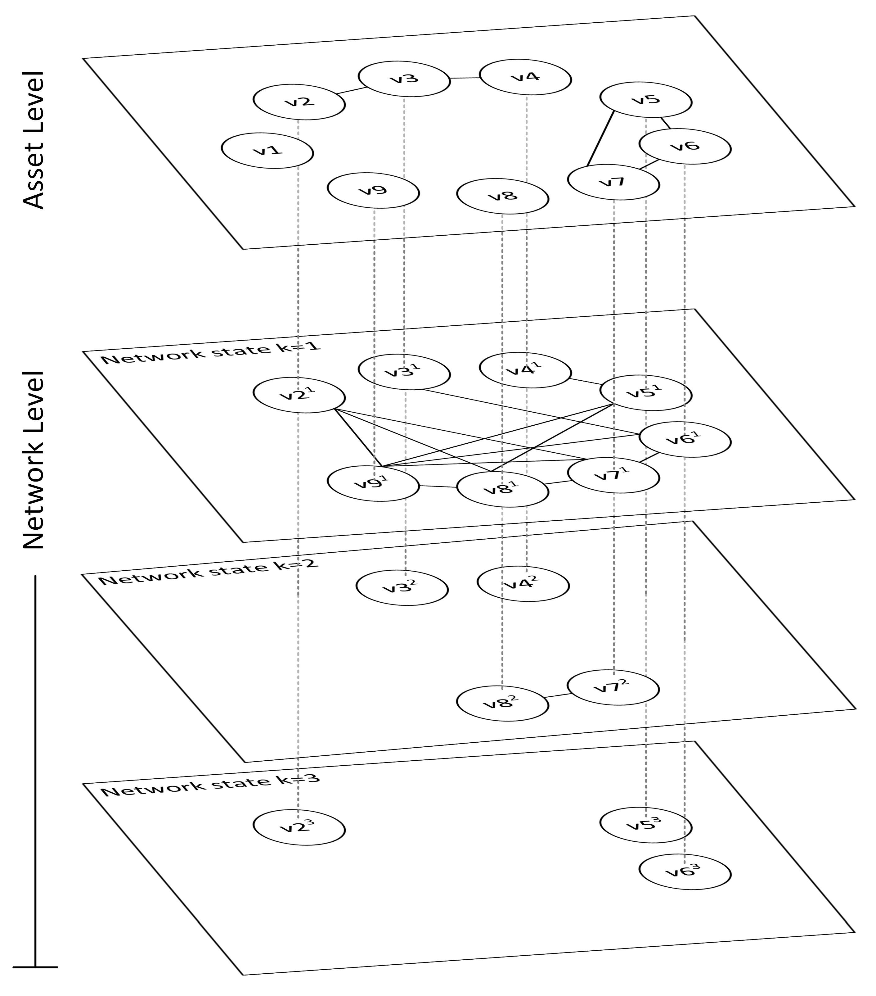
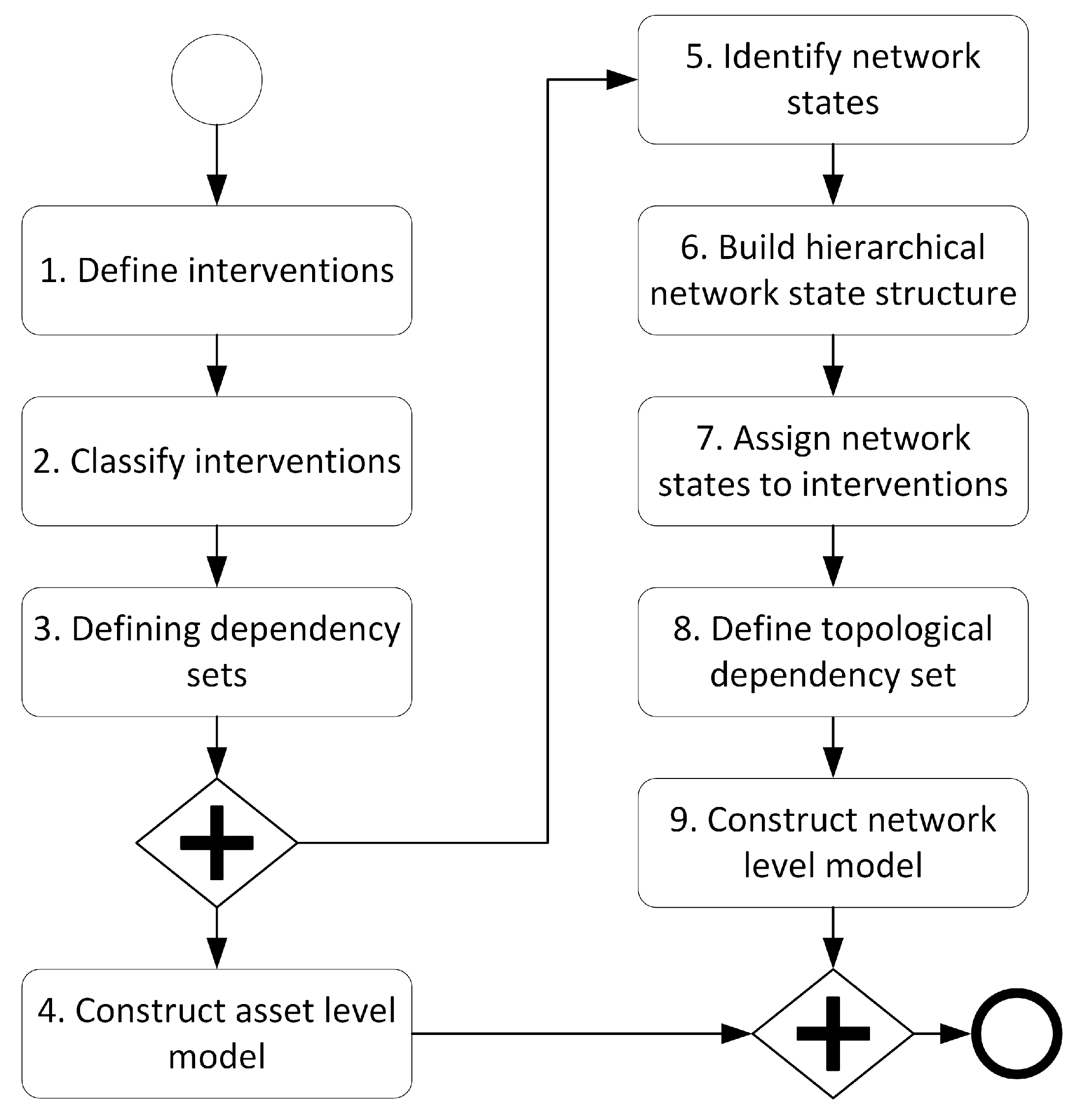
The algorithm to build the system model to model the relationships between the candidate interventions, the intervention costs and the service provided of an intervention program is shown in
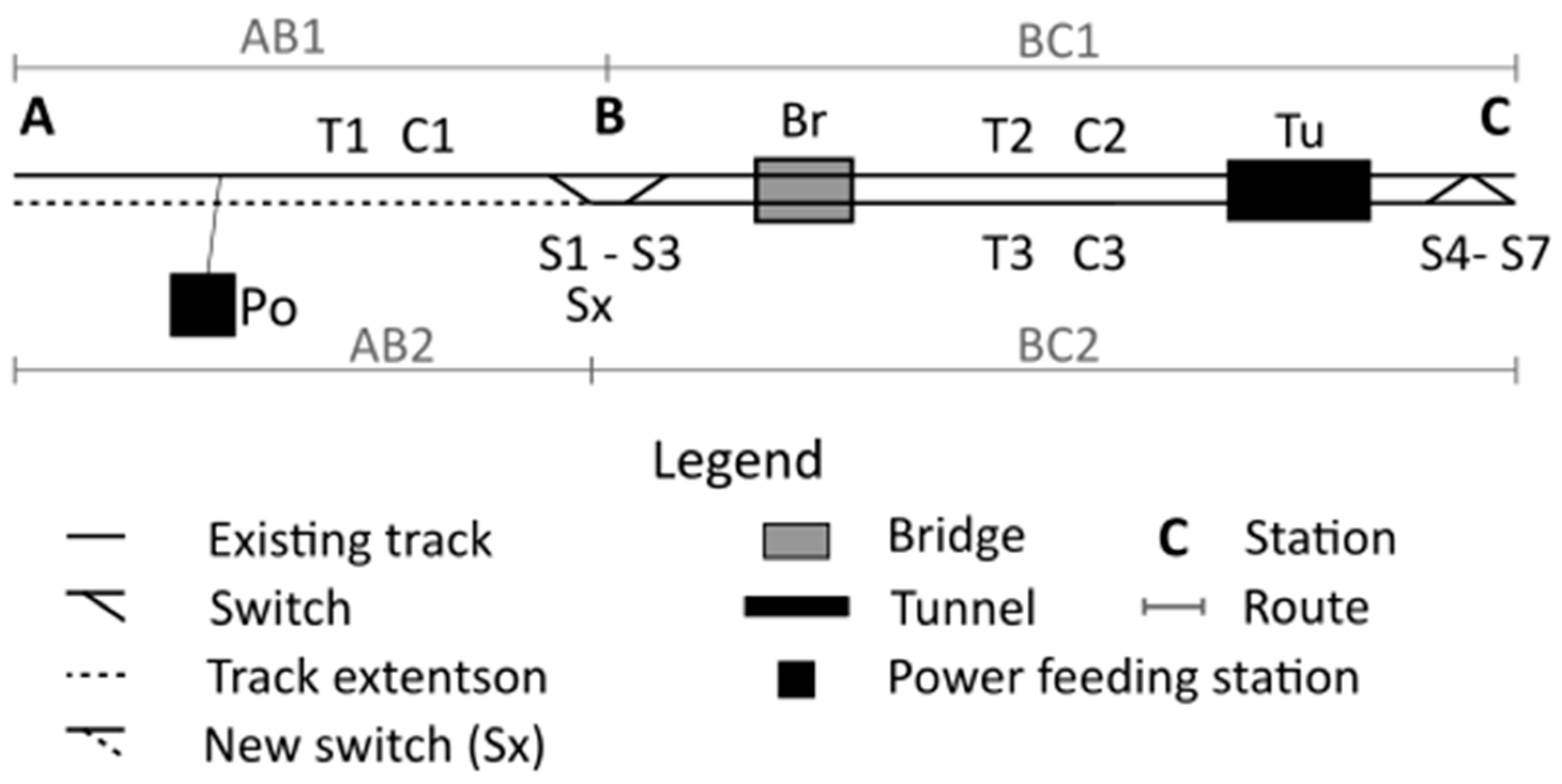
Figure 2, and described in detail in the following subsections with an illustrative example for a railway network, which is shown in
Figure 3. The railway line between stations
A and
C consists of the single-track section
AB and the double-track section
BC. Stations refer thereby to passenger stations. The line consists of assets of different types, i.e., 3 track segments (
T1 to
T3), 7 switches (
S1 to
S7), a bridge (
Br), a tunnel (
Tu), 3 catenary segments (
C1 to
C3), and the power feeding station (
Po). Additional to the existing assets, the extension of the single-track section
AB to a double-track section is considered, which includes switch
Sx as the connection switch in station
B.
4.1. Define Interventions
In the first step, the interventions are defined. An intervention refers to a specific intervention that could be executed on a specific asset. The interventions considered depend on the situation and the asset types considered. The interventions can include maintenance, rehabilitations, renewals, improvements or network extensions, e.g., new assets.
The interventions considered in the illustrative example are shown in
Table 1. The number of candidate interventions is kept at a small quantity while covering a wide variety of assets and interventions. At least one intervention for each asset is considered. The interventions cover maintenance (e.g., track vegetation management), renewal (e.g., bridge renewal), improvements (e.g., tunnel improvement) and extensions (e.g., track extension). The considered interventions are selected in order so that at least one candidate intervention is considered for each intervention type introduced in the second step (see
Section 4.2 for more details).
Table 1 shows the indication of the candidate interventions further used in this paper. For example, the track renewal on track segment 3 is indicated by
T3(
R).
4.2. Classify Interventions
In the second step, the interventions are classified according to their intervention type
. The intervention types
refer to the execution characteristics of the interventions. The five types shown in
Table 2 consider the work process of the interventions, i.e., continuous (I) and local (II to V), the location of the intervention, i.e., within (I, II, IV) and outside (III and V) of the proximity used to provide service, and the effect of interventions on the service provided, i.e., disturbing service (I and III) and not disturbing service (IV and V).
The interventions considered in the example are selected to cover all five types (
Table 1). Track renewal and catenary replacement are interventions of type Ⅰ. They all are executed continuously along the network with maintenance trains requiring track possession and prohibit the execution of other interventions. Switch renewal, bridge renewal, tunnel improvement and the construction of the new switch are interventions of type Ⅱ. They are local interventions requiring track possession at their location. All the interventions so far prevent other interventions to be executed at the same location. The renewal of the power feeder station is an example of a type Ⅲ intervention. It disturbs the operation of the railway network without requiring track possession. Manual vegetation maintenance on the track is an example of a type Ⅳ intervention that requires access to the track for short times, which can be arranged around the normal traffic operation. The track extension excluding the connecting switch is an example of a type Ⅴ intervention that does not affect track possession and the train operation.
4.3. Define Dependency Sets
In the third step, the dependency sets are defined, which are subsets of the candidate interventions describing the dependencies between them. The economical, structural and relevant resource dependencies can be written using such dependency sets. The topological dependencies are considered later in the algorithm.
4.3.1. Economical Dependencies
The set of economical dependencies is a set of unordered pairs of interventions indicating candidate interventions that are economical dependant. In the unordered pairs of ED, the order of and does not matter. In order that two interventions and are economical dependant, (1) the interventions need to have the possibility of being economic dependent, i.e., have shared costs, and (2) the two candidate interventions and need to be in close proximity. The definition of closeness required in condition two depends on the intervention type. If the candidates are of type I, i.e., , the interventions are executed along the asset and economical dependencies exist when the work process does not need to be stopped between the two assets. For example, the renewal of two track segments can share common costs when the two segments are in succession. The two candidates would, therefore, be considered close when the two assets are connected with each other in a topological sense. If the two candidate interventions are of different type, closeness is user defined and depends on the range of the effect of economical dependencies. For example, two switch replacements within the same station can be defined as close, while they are not close when they are located in two different stations 10 km apart.
The illustrative example considers economical dependencies between track renewals on connected assets, track vegetation maintenance on parallel tracks, catenary replacements between connected assets, and switch renewals on switches within the same stations. The complete set can be written as:
4.3.2. Structural Dependencies
The set of structural dependencies is a set of ordered pairs of interventions , where the second intervention is structurally dependent on the first . This means that the dependant intervention is required when the first intervention is selected. In other words, always has to be selected together with , while can be selected with and without .
The example infrastructure consists of structural dependencies between the bridge and the assets on the bridges, i.e., track and catenary, and between the tunnel and the assets in the tunnel. The complete set of structural dependencies of the example infrastructure is
4.3.3. Resource Dependencies
The set of resource dependencies considers the resource dependencies that do not allow the execution of interventions parallel in time. This refers to machinery and work teams that are strictly limited, e.g., only one machinery of a type is available. Resource dependencies that limit the overall selection of interventions, i.e., budget, are not considered in the system model. They need to be considered as constraints when optimising the intervention program within an optimisation model. The set consists of subsets containing all interventions dependent on the same resource
The resource dependencies considered in the example infrastructure are the unique maintenance trains for track renewal and for the catenary replacement. For both type of interventions, only one maintenance train is available meaning that their interventions cannot be executed in parallel due to resource dependencies. The set of resource dependencies of the example infrastructure is
4.4. Construct Asset Level Model
The information gathered in the first three steps allows the creation of the asset level model described in
Section 3.1. Graph
consists of the nodes
representing the interventions
and the edges
referring to the economical dependencies
. Each edge
connecting nodes
and
represents a pair of interventions
that belongs to the set of
, i.e.,
.
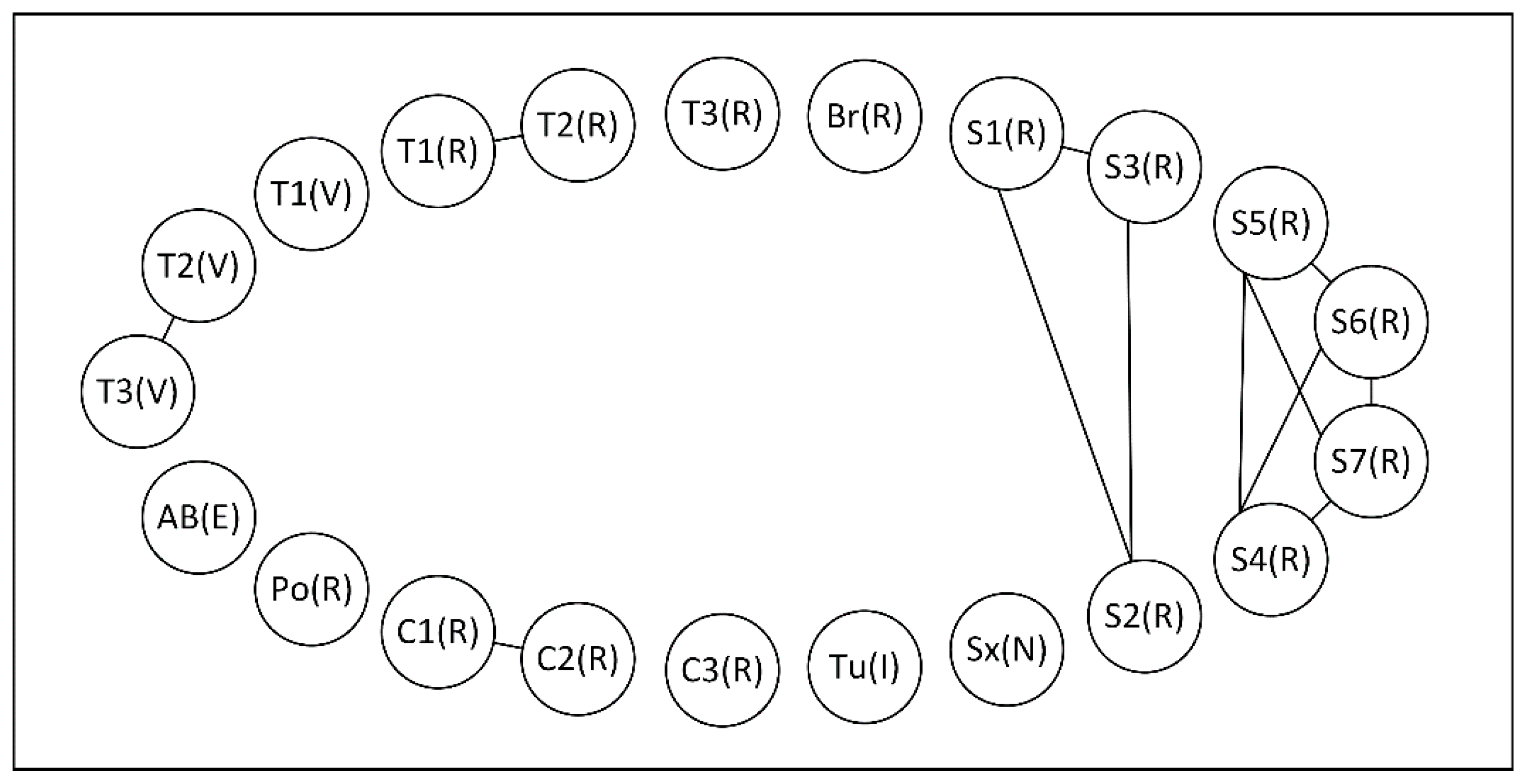
Figure 4 illustrates the asset level model of the example network. Each node represents an intervention. Each edge represents an economical dependency between two interventions. Interventions like bridge renewal
Br(
R), tunnel improvement
Tu(
I)), the new switch
Sx(
N), and track extension
AB(
E) are not connected to other interventions as they have no economical dependencies with other interventions.
4.5. Identify Network States
In step five, all network states are described with which interventions may be executed. The network states define how the service is disturbed by defining the location and extent of the disturbance, e.g., reduced service on a section of the network or a complete shutdown of an entire line. They depend on the infrastructure operation and the network topology.
The line AC of the example railway network shown in
Figure 4 is broken down into sections
AB and
BC. Section
AB consists of one track route, i.e., route
AB1, while section
BC is divided into two track routes based on the possibilities to reroute running trains at switch locations, i.e., route
BC1 and
BC2. For a railway network, it is reasonable to identify the network states based on the station locations since the service is always provided between at least two stations. The identified and considered network states are shown in
Table 3.
4.6. Build Hierarchical Network States Structure
In step six, the hierarchical network state structure is built that defines the hierarchical relation between the different network states. Having two network states , state is considered to be hierarchical below state when the disturbance, i.e., the location and extend, of is part of the disturbance of . For example, a network state that describes the closure of one of two parallel lines is hierarchical below a network state that describes the closure of both parallel lines. The hierarchical network state structure allows to identify the set of all network states that are hierarchical below a certain network state , which is defined as the branch of network state , i.e., . also includes network state itself.
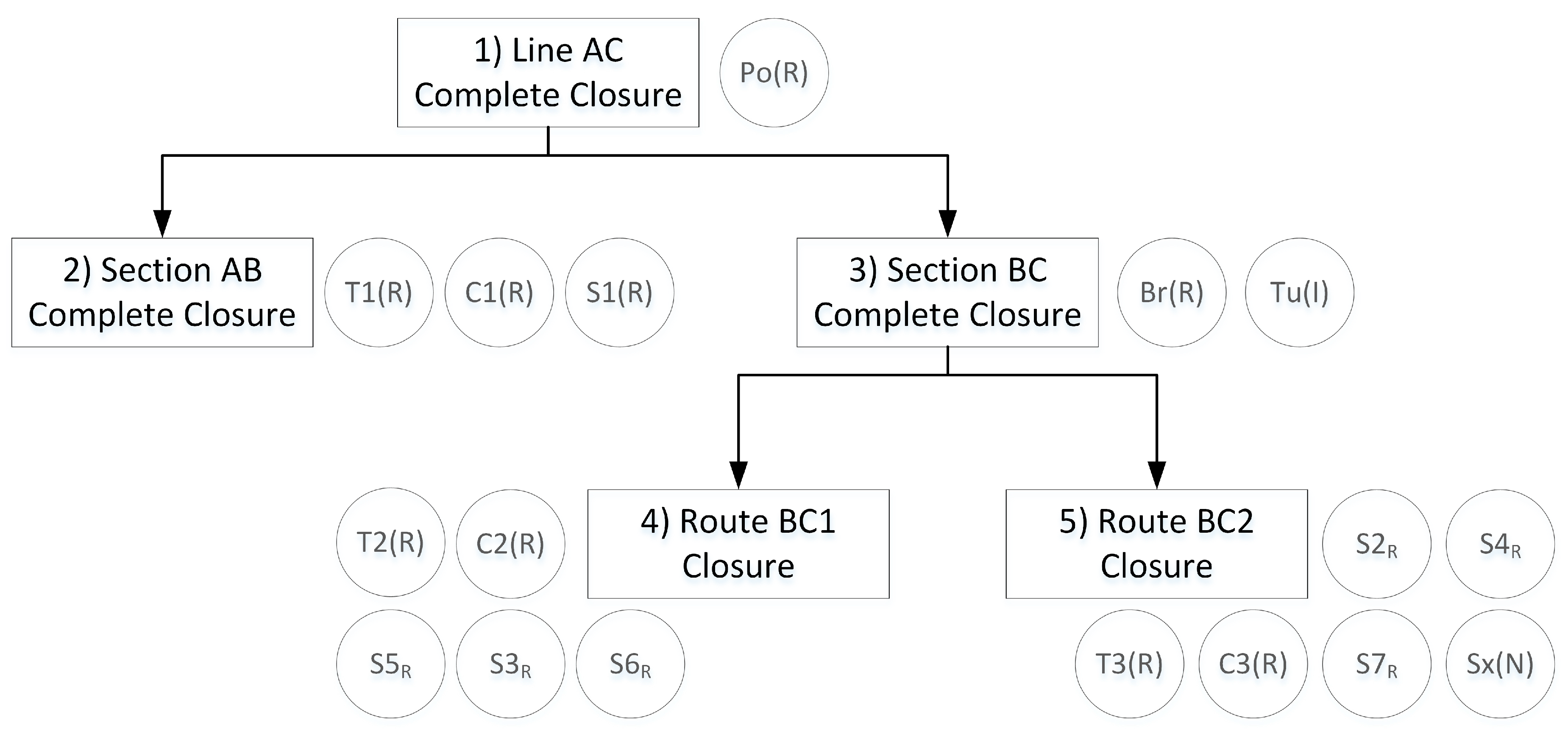
Figure 5 shows the hierarchical network state structure for the example network. In the figure, the network states identified in
Table 3 are shown as rectangular. The arrows identify the hierarchical structure by defining the next lower network states. For example, network state 3
Section BC Complete Closure is above network states 4
Route BC1 Closure and 5
Route BC4 Closure as both of them are part of the complete closure of section
BC.
The branches of each network state are shown in
Table 3. For example, the branch of network state 3 contains network states 3, 4 and 5 as all except 3 itself are below network state 3. The branch of network state 5 consists only of 5 itself as no other network state is below it.
4.7. Assign Network States to Interventions
Having the hierarchical network state structure, each intervention is assigned with its basic network state , which is the lowest network state on which the intervention can be executed. The hierarchical network state structure enables thereafter to identify whether an intervention can be executed under a certain network state, which is true when the network state considered is hierarchical above the basic network state of the candidate intervention.
The assignment of the candidate interventions on the network states of the example network are shown in
Figure 5 by circles. For example, network state 5
Route BC2 Closure is assigned to
T3(
R) as basic network state as this intervention only requires a closure of route
BC2. The assigned network state of candidate intervention
Po(
R) is network state 1 as the renewal of the power feeding station requires shutting down the electricity on the entire line
AC. For candidate intervention
Br(
R), it is assumed that the bridge renewal requires a complete closure of section
BC. Thus, its assigned basic network state is state 3
Section BC Complete Closure. Interventions of intervention types IV and V, i.e., track vegetation maintenance and the track extension, are not assigned with a basic network state since they do not lead to any disturbance.
4.8. Define Topological Dependency Set
In step eight, the topological dependency set is defined. The topological dependency set consists of triplets indicating that interventions and are topological dependent when executed with network state . This means that the two interventions can be executed in parallel. Equation (7) shows the condition that is an element of . First, the basic network state of both interventions, i.e., and need to be in the branch of network state , i.e., . Second, the pair is neither economical, structural nor resource dependent, which would require a sequential execution of the interventions. Third, the interventions have to satisfy one of the following conditions (second line of Equation (7)).
The interventions are both of type I and do not affect the same part of the network. Two interventions and do not affect the same part of the network when there exists an empty union of their network element branches and .
One of the two interventions is of type I and the other of type II, and they do not affect the same part of the network.
Both interventions are of type II.
At least one of both interventions is of type III.
Below, the topological dependency set for each network state of the example network is shown. A candidate
refers to the triplet
.
4.9. Construct Network Level Model
In step ten, the network level model introduced in
Section 3.2 is constructed. The network level is graph
consisting of the nodes
and edges
. This subgraph of
is a multi-layer graph with layer
representing network states.
Node
representing the intervention
executed with network state
only exists when the intervention
can be executed in network state
. This is true when the basic network state of the intervention
is an element of the branch of network state
, i.e.,
.The edge
represents two interventions
and
in network state
that can be executed in parallel at the same time. This are the intervention pairs in the topological dependency set
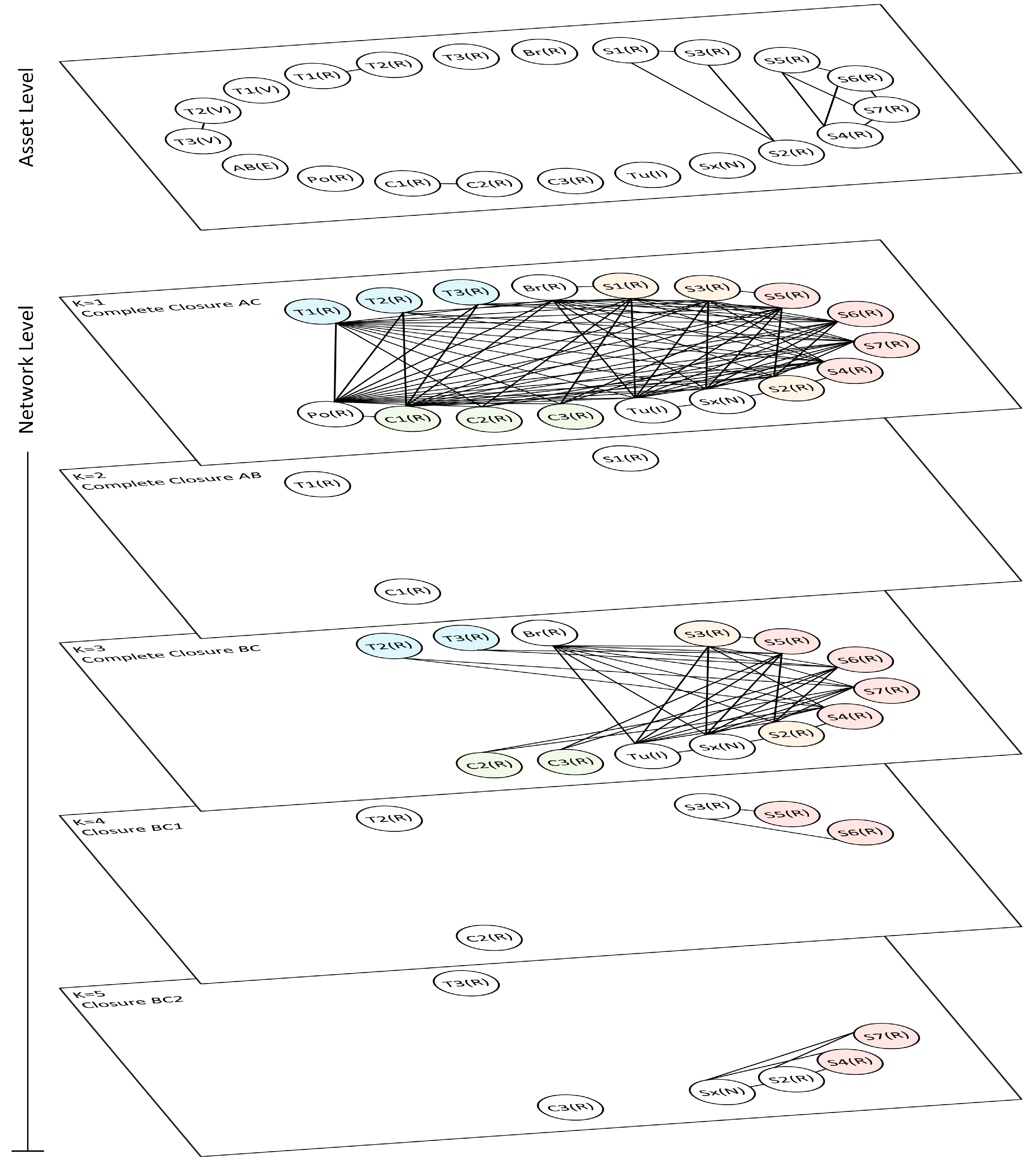
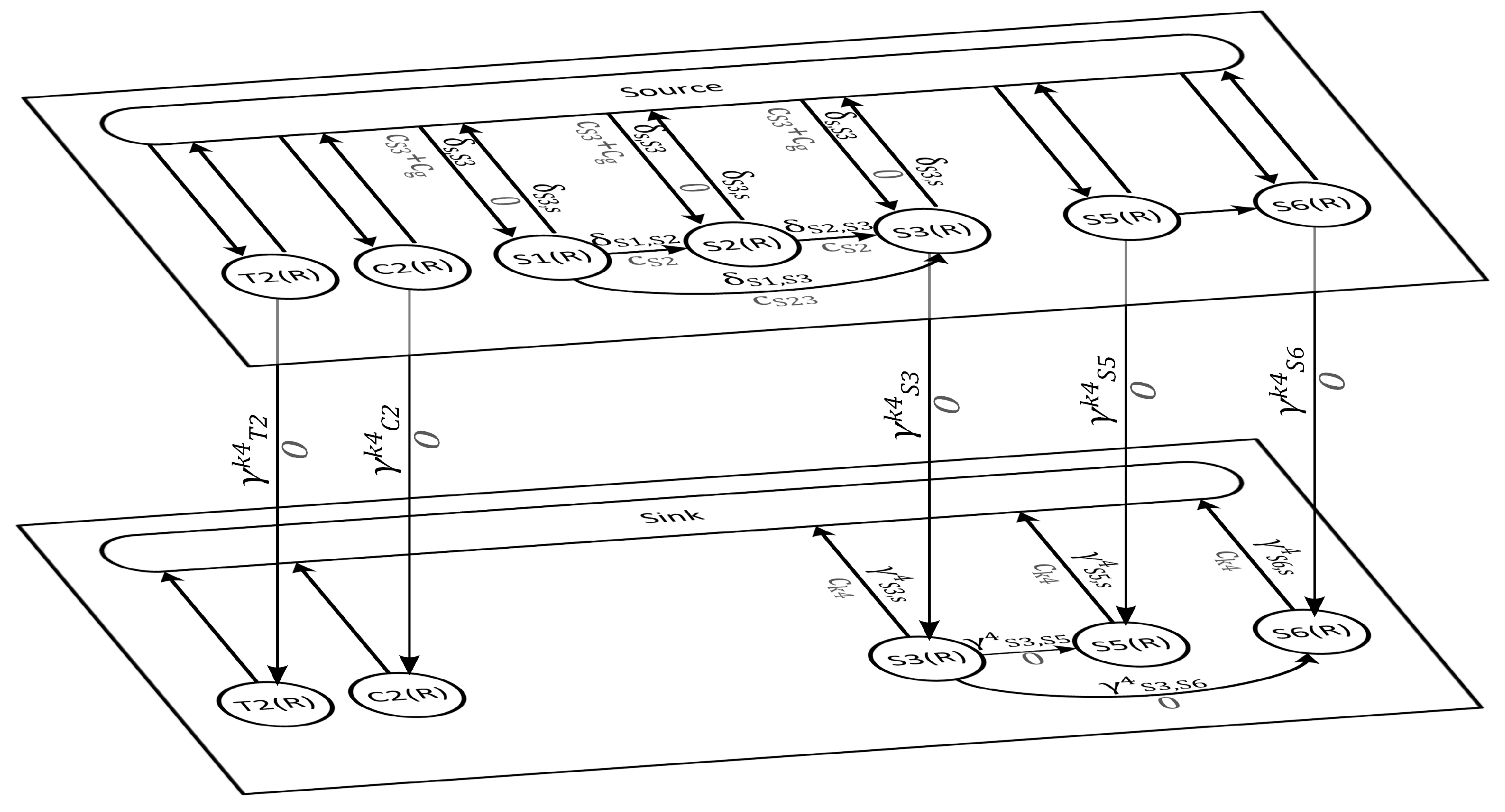
. The network level model of the example network is shown in
Figure 6. The figure shows the graphs of the 5 layers representing the 5 network states together with the asset level. On network state 1, i.e., complete closure of line
AC, all candidate interventions are represented that are assigned by any network state of the branch of state 1 in the hierarchical structure (
Figure 5). These are all interventions on line
AC that lead to traffic disturbance, i.e., are of type I, II or III. Track vegetation maintenance on tracks
T1 to
T6 are not included, as type IV interventions do not disturb the traffic operation.
The edges show all possibility to execute two interventions at the exact same time. For example, T1(R) is connected with Po(R) showing a topological dependency between the two interventions with network state 1. These two interventions can be executed at the same time. The coloured nodes indicate interventions that are either economical or resource dependent prohibiting the parallel execution of these interventions. For example, T1(R) is economical dependant on T2(R) and resource dependant on T3(R), and therefore not connected to any of these nodes by an edge.
Considering the graphs of the other network states,
Figure 6 shows that network states in a lower hierarchical position have fewer interventions that can be executed with them. Network state 2
Complete Closure AB, for example, consists of three interventions that are not connected with each other meaning that all three interventions would have to be executed separately. This means that no possibility exists with which to reduce the duration required, and with it the costs, by executing the interventions simultaneously.
6. Discussion
As outlined in the summary of the system models used in existing research on determining intervention programs, there is room to improve system models regarding the trade-off between the consideration of the complex relationships and the modelling of them in a way that enables the formulation of optimisation models that can be solved without heuristics. The new bi-level graph theory type of system model proposed does this through the improved modelling of the complex relationship between interventions, interventions costs and the service provided by infrastructure networks when determining intervention programs. The graphs of the asset and network level enable accurate consideration of the economical and topological dependencies between interventions, which influence the intervention costs and the effects on service associated with an intervention program. This overcomes the limitation of the linear combination, group state and existing graph theory system model that all simplify or even neglect these complex relationships. The combination of graph theory and a bi-level consideration in the proposed system model enables to consider properly the relationships while they can mathematically be described in linear form. This enables, different to optimisation models constructed using existing reliability block diagram or bi-level system models, to construct optimisation models using mixed integer linear programs that can be optimised without the help of heuristics. Overall, the type of system model proposed (1) is suitable for the estimation of the intervention costs and the effects on service associated with an intervention program, (2) does not neglect or overly simplify the relationships between interventions, interventions costs and the service provided by infrastructure networks, and (3) enables the construction of optimisation models using mixed integer linear programs that can find the optimal sets of interventions without the help of heuristics, e.g., with Branch-and-Bound and Simplex. This reduces infrastructure managers need to qualitatively adjust the results of current algorithm proposed intervention programs, and, therefore helps in the process of digitalisation of railway infrastructure management.
The asset level enables the estimation of the asset level costs, i.e., the costs for material, labour and equipment, based on economical dependencies between interventions, i.e., shared costs, and the managers’ decision about which interventions to be included in the intervention program. The network level model enables the estimation of the network level costs, i.e., costs for work zones and due to traffic disruption, based on the determination of the longest duration required to execute a selected combination of interventions. For example, considering intervention
S3(
R),
S5(
R) and
S6(
R) with network state 4 (
k = 4) in
Figure 6. Intervention
S3(
R) can be executed in parallel with interventions
S5(
R) and
S6(
R), i.e., are topological dependant. Interventions
S5(
R) and
S6(
R), however, need to be executed in series, i.e., are economical dependent. The network level model enables to determine the duration required to execute the interventions by enabling to subtract the duration of
S3(
R) executed in parallel with either
S5(
R) or
S3(
R) dependent on which of the interventions are actually selected to be executed with network state 4. The existing system models using linear combination, group states and graph theory would either sum the durations or require a pre-defined definition of which duration to be considered.
Further, existing system models based on group states and reliability block diagrams are limited in the consideration of the variations in the network states during the execution of an intervention program. The graphs used in the system model proposed enable the consideration of the variation in the network states dependent on the decision which intervention to execute and with which network state. For example, an intervention program could consist of executing interventions in all five network states considered in the. Every change in the decision about the intervention program may change the network states with which the interventions are executed significantly, while the system model remains the same and enables to estimate the costs and impacts on the service provided of the changed intervention program.
In order that system models of this type can be used in different situations, a systematic and consistent algorithm to build them is provided. The algorithm uses an intervention classification and a hierarchical network state structure to build the graphs. Both the classification and the structure enable the algorithm to be used for different asset types and interventions. The use of the algorithm on the example network demonstrates the ability of the algorithm to be used on networks with assets and interventions of different characteristics, e.g., a railway infrastructure consisting of tracks, switches, bridges, tunnels and an overhead power supply system, as well as the consideration of maintenance, renewal, improvement and extension interventions. The algorithm, and with it the representation, can be used in all cases, as long as the candidate interventions can be classified according to the classification scheme. The use of the algorithm to develop the system model for the example network also shows that the intervention classification and the concept of hierarchical network state structure is applicable for railway infrastructure networks. Further work is required to investigate the use of the algorithm on infrastructure networks of other types, e.g., for road, water or energy infrastructure networks.
7. Conclusions
This paper proposes a new bi-level graph theory type of system model to improve the modelling of the complex relationship between interventions, interventions costs and the service provided by infrastructure networks required to determine intervention programs.
The proposed type of system model (1) enables the estimation of the intervention costs and the effects on service associated with an intervention program, (2) properly models the relationships between interventions, interventions costs and the service provided by infrastructure networks, and (3) enables the construction of optimisation models using mixed integer linear programs.
The system model uses graphs to model both, the asset level costs, i.e., costs of the execution of the interventions, and network level costs, i.e., the disturbance in the service provided by the infrastructure. The asset level enables the consideration of economical dependencies between candidate interventions, i.e., shared set-up costs. The network level considers the different network states with which interventions can be executed. A network state describes thereby a specific way how the infrastructure is operated considering a specific set of closures or shutdowns in the network. The graph of the network level enables the modelling of the duration of each network state required during the implementation of the intervention program considering the topological, structural and resource dependencies. They define whether interventions can be executed parallel in time or whether interventions require a sequential execution.
Further, the paper proposes an algorithm that allows the building of the system model independently of the asset types considered. The algorithm uses a specific intervention classification that classifies the intervention into five different types dependant on how they affect the service provided by the asset during the intervention execution. This classification enables the algorithm to be applicable for a combination of different types of assets, e.g., railway track, bridges, tunnels and catenaries, and for different interventions, i.e., maintenance, rehabilitation, renewal, improvement and extension.


