Procedure for the Identification of Existing Roads Alignment from Georeferenced Points Database


Department of Civil, Constructional and Environmental Engineering, University of Rome La Sapienza, Via Eudossiana 18, 00184 Rome, Italy
*
Author to whom correspondence should be addressed.
Infrastructures 2021, 6(1), 2; https://0-doi-org.brum.beds.ac.uk/10.3390/infrastructures6010002
Submission received: 12 November 2020
/
Revised: 16 December 2020
/
Accepted: 22 December 2020
/
Published: 24 December 2020
Abstract
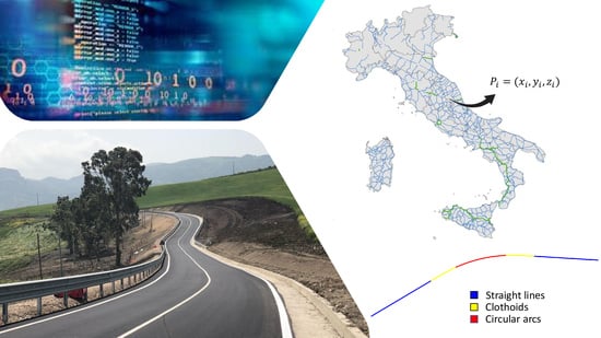
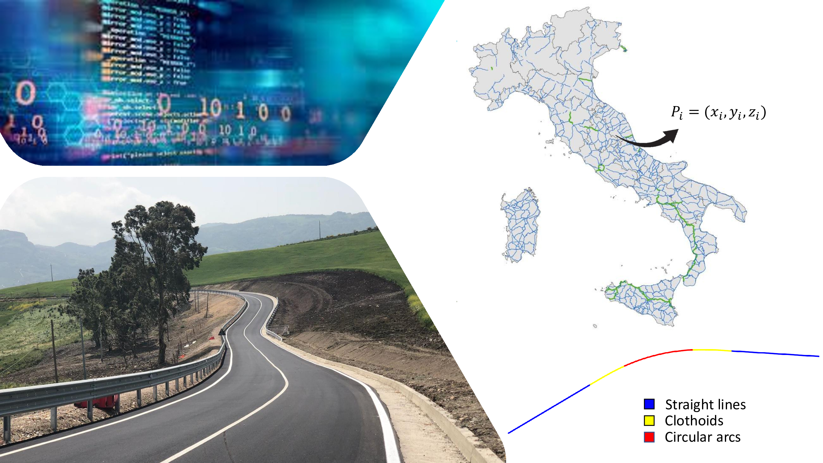
:The aim of this research is to look for an automated, economical and fast method able to identify the elements of an existing road layout, whose original geometric design could date back to distant ages and could have undergone major modifications over the years. The analysis has been directed towards the Italian two-lane rural roads; the national public company ANAS made available its graph, obtained from high-performance surveys, that represents about 90% of these roads’ network. The graph is made up of a collection of georeferenced points but does not recognize or describe the geometric elements making up the roadway. Consequently, it has been necessary to design and develop an original procedure, subsequently implemented in a programming platform, able to identify the characteristics of the several parts, which constitute the reference axes of the existing roads. This research focuses on the horizontal geometry assessing the coherence, consistency and homogeneity of the roads’ layout, through the ex post application of the regulatory model for the design verification. If road sections are identified in which some conditions are not significantly met, further investigation should be conducted in order to ensure road safety and to plan any road upgrading activities.
1. Introduction
1.1. Context and Aim of the Work
The safety assessments for newly built roads can be carried out according to the guidelines of the design standards. In Italy, specifically, the Ministerial Decree dated 5.11.2001 [1], referring back to the road classification of the Highway Code [2], defines the constructive, technical and functional characteristics of each type of road; with regard to these features, it imposes prescriptions for the design and verification of the geometric elements and their composition, so that the road users’ movement takes place regularly and safely.
The verification of the design accuracy includes the road consistency examination. The road consistency is the characteristic of the infrastructure that makes it suitable to meet road user expectations and implies that the geometric successive elements are coordinated in order to produce harmonious and homogeneous driver performance and to not generate incorrect and, sometimes, unsafe driving behavior [3,4,5].
The rules that guide road design should ensure that a driver is spontaneously induced to adopt a driving behavior that is congruent with the real characteristics of the road. It is the case of the “self-explaining roads” [6,7], which are defined as roads where drivers perceive and recognize the features of the infrastructure they are driving on and “instinctively” know how to behave [8]. Since the driver’s behavior is directly related to the perception of the route he/she is following, a designer should make the road as readable as possible, so as to guide the user in the behavioral choices to be adopted, suitable to deal with even the most dangerous situations [9,10,11].
Many studies have found that some design choices, violating the user’s expectations, can negatively affect his/her behavior [12,13,14,15], by inducing the disoriented driver to change his/her usual driving choices and leading him/her to have risky driving behavior.
The inadequacy of the technical characteristics of the road can be detected under several aspects, including, for example, unsuitable adhesion values of tire-asphalt pavement interface to guarantee the transfer of dynamic actions, geometric horizontal alignments design or conditions of the environment surrounding the infrastructure insufficient in ensuring a correct perception of the route, especially for occasional users. Design, construction, but above all maintenance problems are often the cause or contributing cause of high levels of accidents on many road networks.
Therefore, it is necessary to investigate in more detail what the role of the infrastructure may be in the occurrence of accidental events, in order to assess what type of countermeasures can be implemented to ensure higher safety standards.
In particular, in order to be conducted, evaluations related to the consistency of the technical characteristics of existing roads, require data that correctly represent the geometric characteristics of the infrastructures; such data are often not accessible, not updated or do not have the accuracy and precision required to perform the analysis to be carried out.
In light of the above, the identification of the plano-altimetric geometrical characteristics of the existing roads is still a topic of great interest in the field of civil and transportation engineering. Considering these problems, the objective of this research is looking for an automated, economical and fast procedure able to identify the elements of a road layout belonging to an existing and operating road network. In particular, the horizontal geometry—and, more specifically, the continuous trend of curvatures—is especially needed in order to perform the ex post application of some standard design rules and assess the coherence, consistency and homogeneity of the road infrastructure.
There are no shared and reliable methodologies that establish how this activity should be carried out, for the purpose of performing road safety analyses and for the maintenance of the infrastructure. Although much research has presented techniques and procedures suitable to obtaining useful data from surveys, no methods are available for the extraction of the reference axis (it means a continuous and coordinated line, composed by basic elements mathematically described, like in the design process of a new track) of an existing road section. Thus, the aim of this work and the proposed contribution to the state of the practice is to overcome the described lack.
1.2. State of the Practice
In general, in order to overcome the lack of information about the existing road networks, a lot of energy has been spent in research aimed at obtaining the geometry of the compositional elements of the layout from different sources. Various attempts were made to obtain information regarding the horizontal and vertical alignment both from aerial and satellite georeferenced images, both from road maps of geographic information systems, and from data collected with positioning sensors on mobile systems and vehicles.
There are many road geometry relief techniques to date, which can be divided into static and dynamic ones, depending on the instrumentation used to obtain the data.
Among the static procedures, the following may be enumerated:
- -
- -
- Automatic identification of road geometry from digital vector data [18].
Among the dynamic ones, on the other hand, it is worth mentioning:
- Detection systems using mobile mapping system (M.M.S.) technology. These are widely appreciated both for their versatility and for their low operating costs. In general, M.M.S. are made up of vehicles equipped with different instruments, properly integrated with each other: a satellite navigation device, an Inertial Navigation System (INS) and an odometer [19,20,21,22]. In specific cases, the “Digital Highway Data Vehicle” (DHDV) has been used, an integrated system through which three Euler angles, the driving speed and the vehicle acceleration were measured to perform the survey in a rigorous way [20,23]. Another instrumented vehicle able to collect pavement condition and asset data and not only geometric information is the van automatic road analyzer (ARAN) [24].
- Global Navigation Satellite System (GNSS) with GPS receivers mounted on trains [25,26,27] or vehicles travelling at almost constant speeds, instrumented with vertical gyroscopes and gyro compasses able to provide information on the vehicle positions (x, y, z coordinates) and orientations (angle of pitch, roll and yaw) [28,29,30,31,32]. In some cases, vehicle positions have been recorded via smartphone [33].
The described techniques are generally efficient and valid for acquiring a dataset but, once the necessary points for the definition of the road geometry have been collected, there comes the need to develop a rapid and economic procedure that allows to easily and precisely obtain the geometric definition of the plano-altimetric road layout that should be mathematically formalized through simple and continuous geometric elements.
The above-mentioned studies and the proposed techniques, in fact, are able to obtain points and to determine the coordinates of the track, but they do not manage to define a continuous curvature graph (or a continuous reference line), which is useful to conduct safety evaluation by means of the ex post application of the design verifications. Only in some cases, they can efficiently identify circular curves with their radii and straight lines, but they cannot represent the reference road axis in the traditional design way as a succession of straight lines, circular arcs and clothoids.
Over the years, multiple algorithms, able to identify in an automated way the circular arcs and the straight lines, have been built; the most successful method is that of the least squares fitting of the points of the road axis. The most widely used and easily implementable algorithm is the least squares circle fitting, able to estimate radius, angle at the center and arc length with high accuracy; as can be seen in Figure 1, it can minimize the deviations between the computed curve and the original points [34].
The least squares regression method is a technique aimed at determining an analytical function that approximates a set of values without necessarily passing through the points themselves. In fact, if the data come from experimental measurements and are, therefore, affected by measurement or instrument errors, or if the data quality is not very accurate (few significant figures), then it is appropriate to approximate to least squares rather than interpolate. In particular, the function found must be the one that minimizes the sum of the squares of the distances between the points and the plotted curve [35].
As an implementation of the aforementioned algorithm, an iterative least squares circle fitting algorithm has been proposed, which iteratively searches for circumferences approximating the available data, changing the center and radius of the arc from time to time, until the smallest possible differences between the input data and the originated output are achieved [28]. Another similar method, useful for searching the characteristic parameters of horizontal curves, generates from the calculation of each circle that can be drawn using all the triplets of non-aligned points, reducing iteratively the distance between the circle and the complete set of points, using a minimization method [36].
In general, the algorithms developed through the least squares fitting method have tried to evaluate the reliability and accuracy of the results obtained, considering the errors due to the surveying GPS instrumentation [32,37,38].
Other approaches defined by data collected from inertial measurement units fitted to road vehicles have also been used for radius measurement, including the kinematic method, the geometry method, the lateral acceleration method and the chord offset method [20,39]:
The kinematic method plans to use the longitudinal speed (v) and centrifugal acceleration (a) values, directly obtained from the dataset provided by the vehicle, according to the following formula:
The geometry method involves linear approximation of the vehicle’s trajectory between one measurement point and the next one—linearization made possible by the high data sampling frequency—and calculates the curve radius through the reciprocal of the curvature:
The lateral acceleration method uses the data of super-elevation, side friction factor and speed to calculate the corresponding radius:
According to the chord offset method, the chord length (L) and the offset between the chord and the arc midpoint (M) are measured through the vehicle’s trajectory; using these parameters, it is possible to calculate the radius of the curve:
In order to identify of the starting and ending points of the circular arcs; instead, the heading angle trends have been studied and their linear variation has been determined [20,39].
Finally, it is worth mentioning that several authors have used a completely different method from what was exposed so far to recreate the road geometry; this method involves the interpolation of raw data, acquired to identify the road layout, through polynomial curves and/or splines [29,30,40,41].
In contrast to some previous research, which are based on the B-spline approximation [30,42,43], the proposed method utilizes a data fitting process. The least square regression is an optimization technique that allows to find a function, represented by an optimal curve, that is as close as possible to a set of data. Other similar procedures have been implemented in these years to automatically identify all horizontal geometric elements and produce recreated alignment geometry for existing roads and railways [29,44,45].
2. Materials and Methods
As anticipated, the objective of the analysis entails in the definition of a methodology able to recognize the reference axis, which means the road layout composing elements as a succession of straight lines, circular arcs and clothoids. This is important and necessary for a more general purpose, which consists in the preventive safety evaluation offered by existing roads, through procedures based on the verification criteria of safety conditions referred to the road geometry.
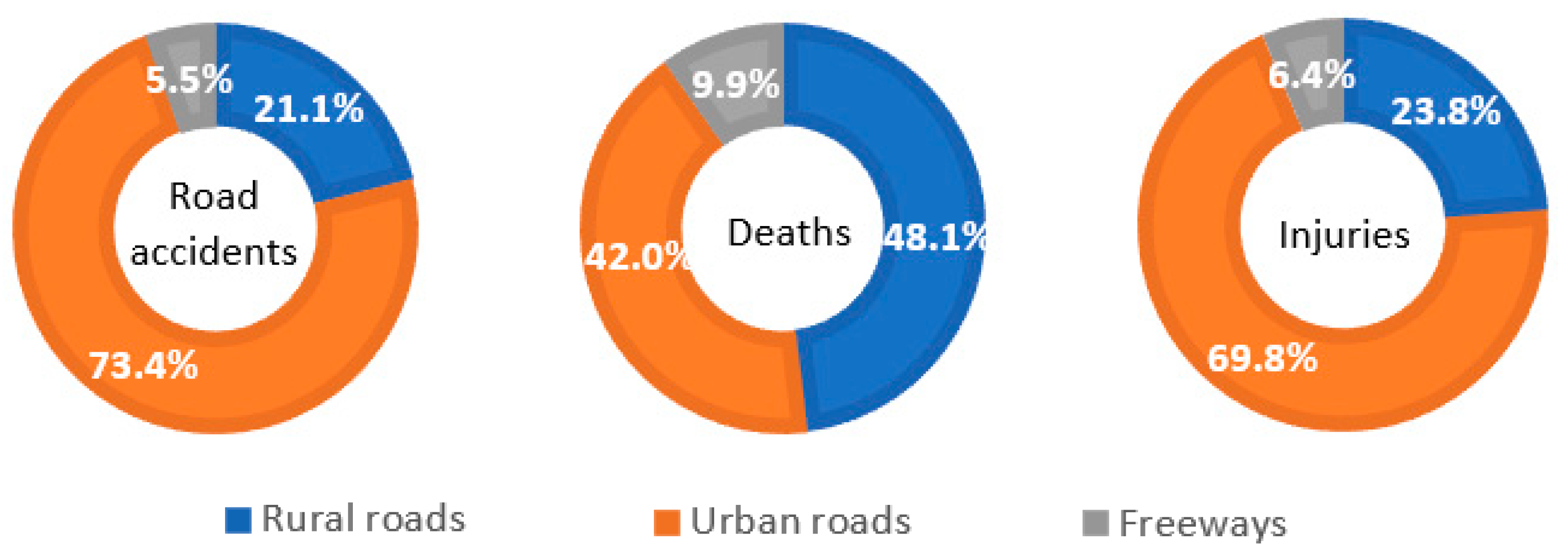
It should be noted that, for example, on Italian roads in 2018, road accidents with injuries to persons were 172,553, with 3334 victims and 242,919 injured (see Figure 2). Accidents and injuries are progressively decreasing on urban roads and freeways, while they are increasing on rural roads.
Given the high accident rate found on single-carriageway rural roads, which are more suitable for studying and understanding the behavior of users in relation to the characteristics of the road, it was decided to focus the research on single-carriageway highways outside urban perimeters.
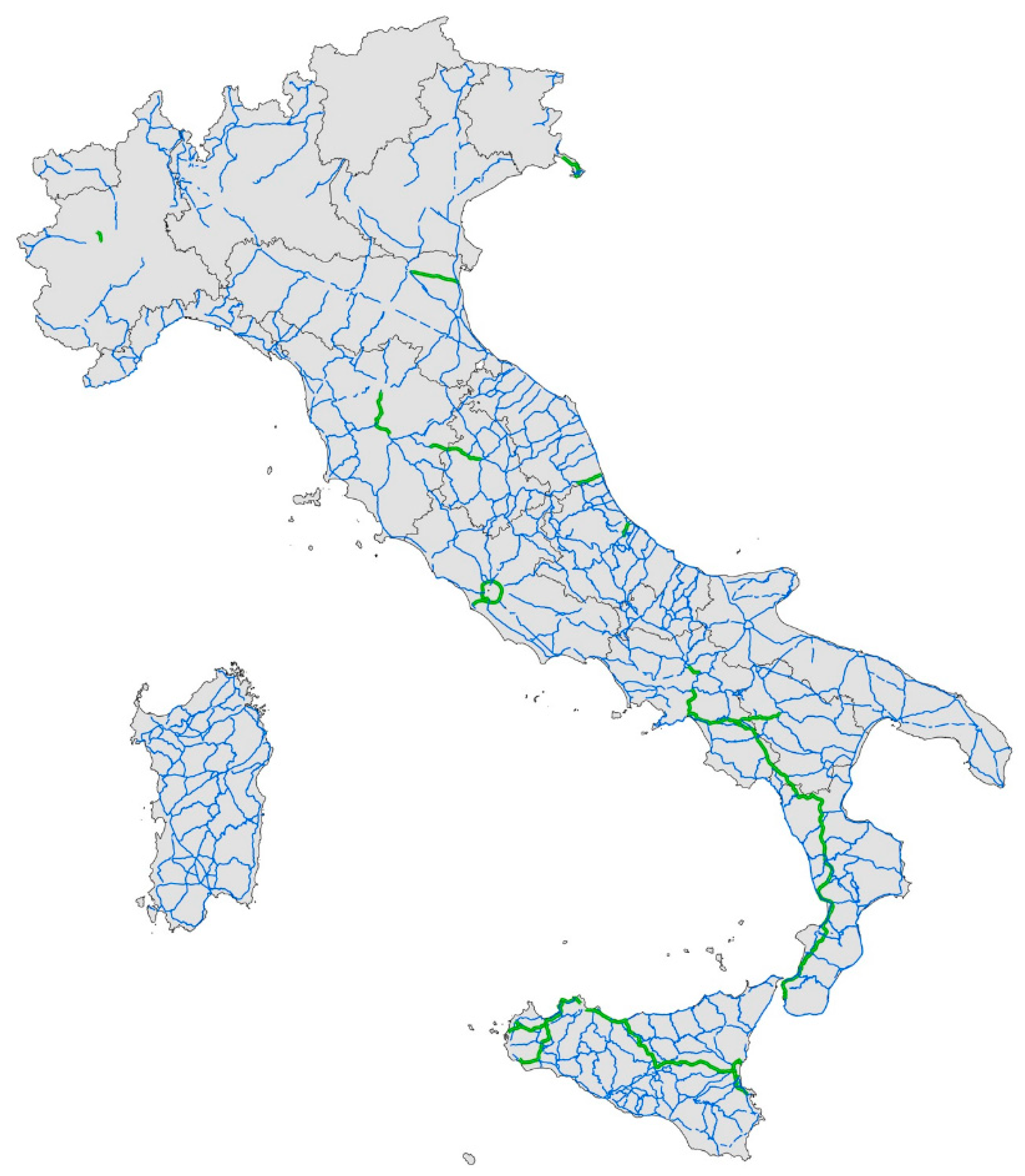
Since the Italian state roads are spread throughout the national territory and about 90% of this network is managed by the company ANAS S.p.A., the choice of the road network to analyze has fallen on the roads managed by this company, shown in Figure 3.
The company ANAS S.p.A. has shared with the authors its road graph, realized by means of high-performance surveys and composed of three-dimensional geographical coordinates. The network graph is, therefore, made up of georeferenced points, but it does not recognize or describe the geometric elements making up the road. Thus, it was necessary to design and develop an original procedure, subsequently implemented in a programming platform, aimed at identifying the different geometric elements that constitute the planimetric road layout.
Therefore, the research essentially consists of a new approach proposed with the aim to reconstruct the horizontal road alignment by using traditional design elements such as straight lines, circular arcs and transition curves.
The first difficulty met has been the processing of a huge amount of raw data, specifically the georeferenced points in space. The first research step has been looking into filtering and sorting the vertices of the road graph to obtain an ordered set of geographical coordinates to be connected.
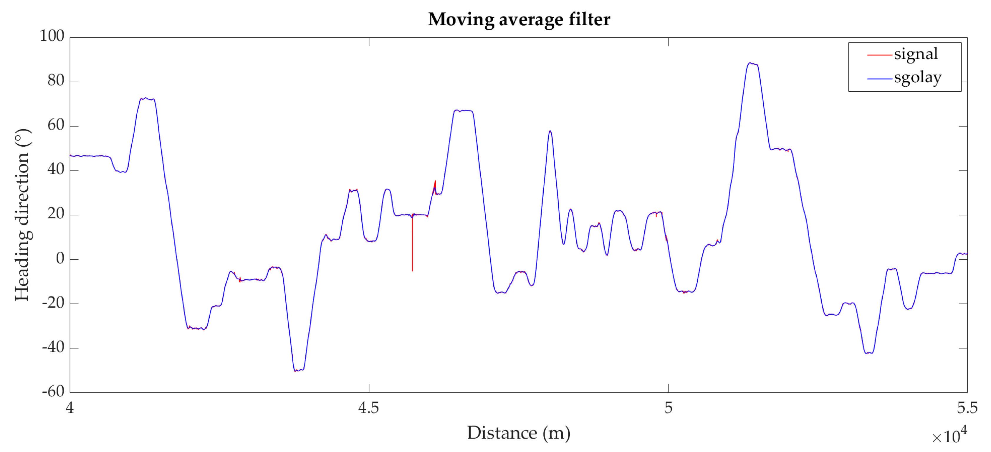
Once the heading direction graph was constructed, it has been necessary to clean the data from repetition and inaccuracy and then smooth the resulted line through the application of a moving average filter, as the values were affected by measurement or instrument errors.
The Savitzky–Golay filter used is a digital low-pass filter that allows to make the data trend more continuous; it is applied to a series of data points in order to decrease the signal noise without deforming the signal. The subsets of consecutive data points are fitted using a low order polynomial with linear least square method, so the convolution of all the polynomials is then obtained [46]. The data, having a set of n {xj, yj} points, where j = 1, 2, …, n, and x is an independent variable, whereas y is an observed value, can be represented with a set of m convolution coefficients Ci; the effect of convolution can be expressed as a linear transformation:
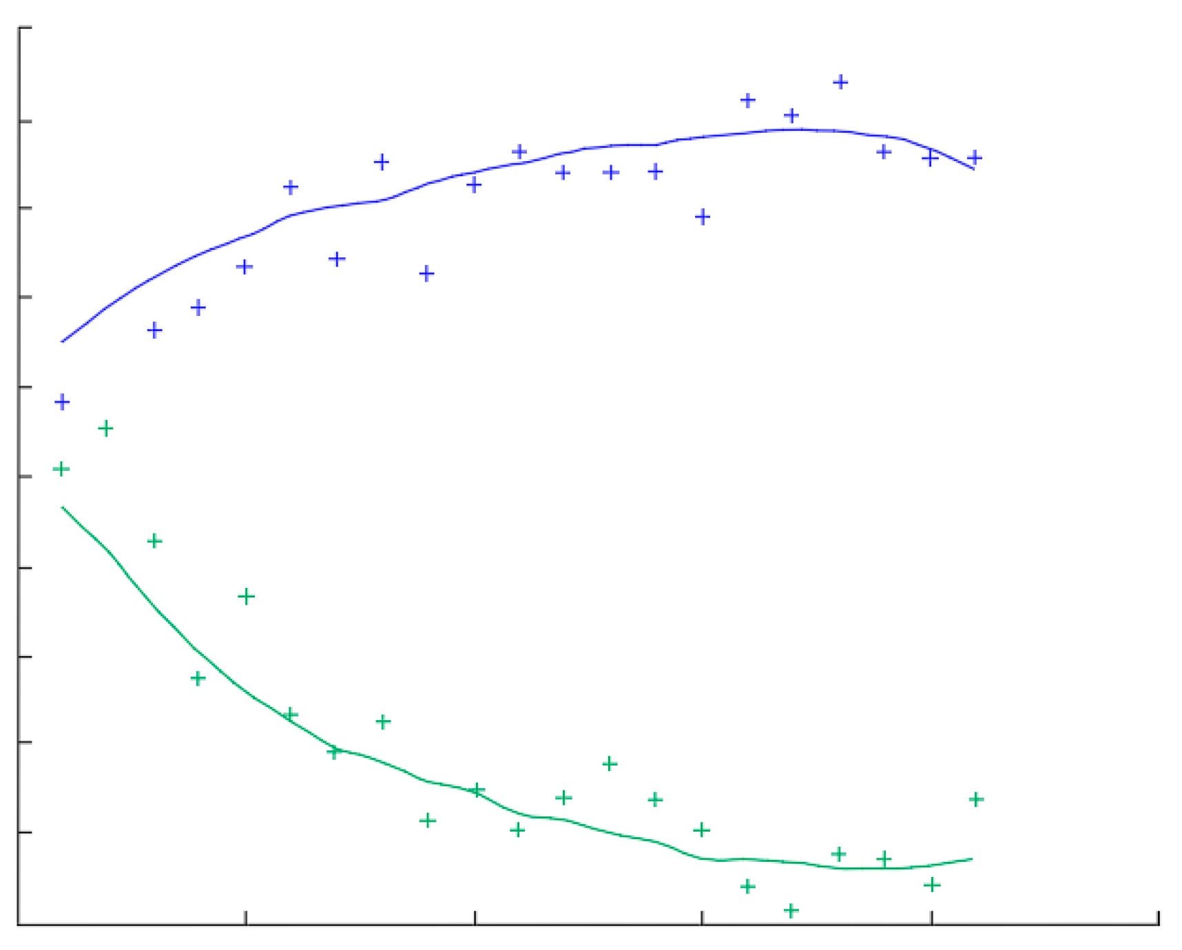
Three inputs are necessary to execute a Savitzky–Golay filter: the signal (x), the polynomial order (k) and its frame length (f); in Figure 4, an example can be seen.
Consequently, a data mining effort has been made to write a code able to automatically approximate the heading direction signal and generate a new trend, through which it has been easier to search for the starting and ending points of the sections with zero curvature.
Subsequently, using the vertices falling within the starting and ending points of each constant curvature element, a least square regression has been implemented in a different code, in order to automatically find centers and radii of the circular arcs, analyzing from time to time the deviation standards.
The optimal values of the original variables x, r can be recovered from the formulae:
Once the geometrical parameters were known, two other programming codes have been written to construct in an automatic and rapid way the curvature graph and the design speed profile, according to the Italian road design guidelines.
This procedure will be described below and Highway n. 4 (S.S. n. 4) will be reported as a case study.
3. Results
The main obtained results refer to the application to the case study of the “Strada statale n. 4 Via Salaria”. This is an Italian state highway (HWY); it is a single carriageway highway for most of its route, presenting one lane per each travel direction, but it falls into the category of dual carriageway urban road in its first part (near to Rome city center). It, therefore, follows that this infrastructure is characterized by many various geometrical elements, changing gradually from urban highway to mountain road.
Once the graph of the road network has been acquired form the company ANAS, the 3D geographical information of the road of interest has been extrapolated, in terms of x, y and orthometric elevation coordinates. Thanks to the east and north coordinates in the WGS 84 UTM zone 32N Reference System, and the elevations in meters above sea level (m.a.s.l.), the planimetric and then altimetric layout of the road have been reconstructed.
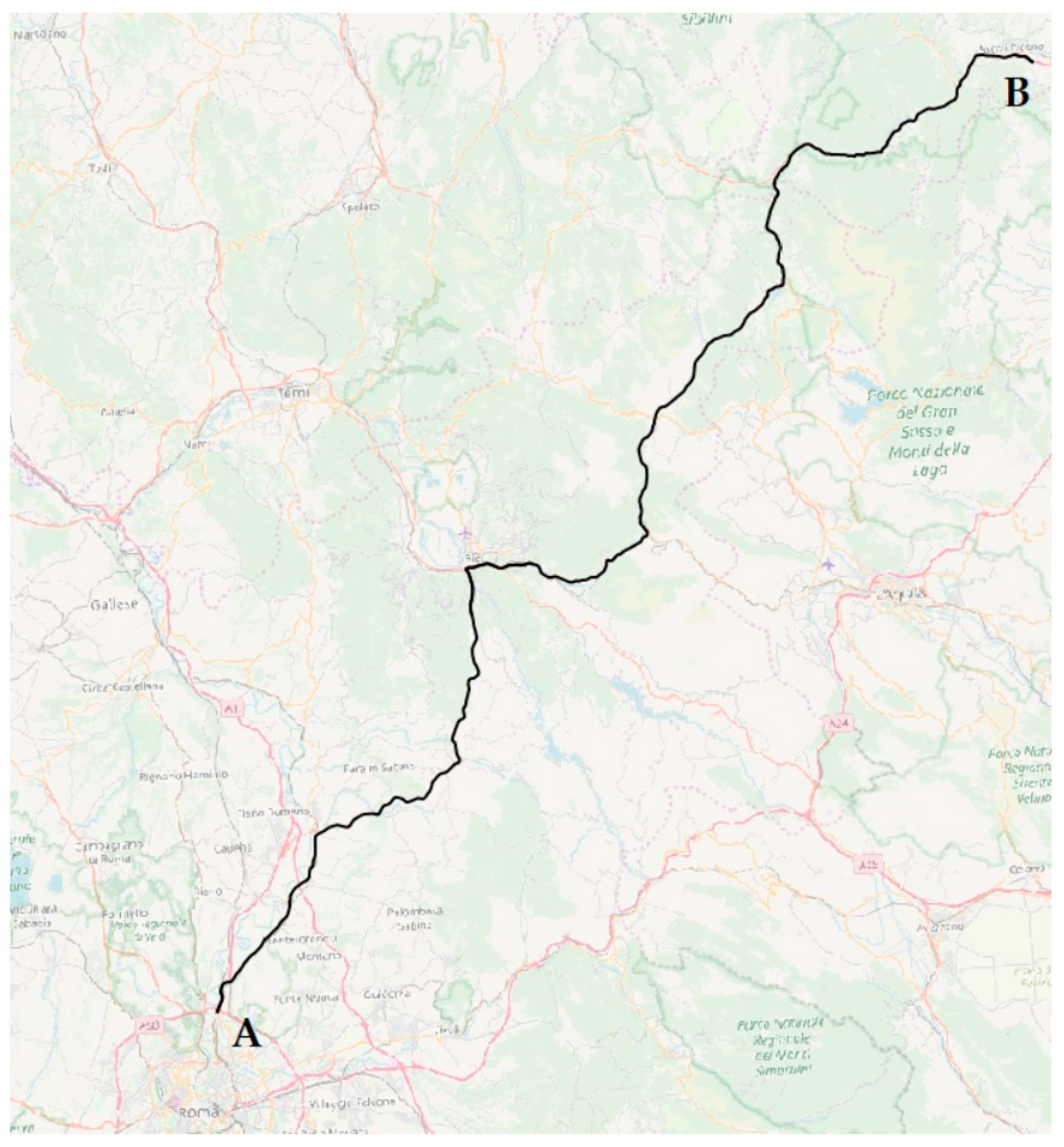
Conventionally the direction of the distance has been taken from point A to point B, linking Rome to Ascoli Piceno, as it can be seen in Figure 5:
The plan reconstruction, as a succession of straight and curved elements, has been carried out in stages through the implementation of a programming code.
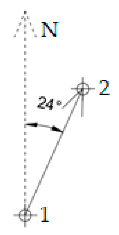
Initially, a denser discretization of the axis was carried out, measuring the distances between two consecutive vertices and dividing the segments longer than 6 m. For each point the Cartesian coordinates, the elevation, the identification code, the azimuth of the segment linking the i-th point to the next one (see Figure 6), the slope (m) and the y-intercept (q) of the straight line passing between the 2 above points, the partial length and, lastly, the distance have been tabulated, as shown in Table 1.
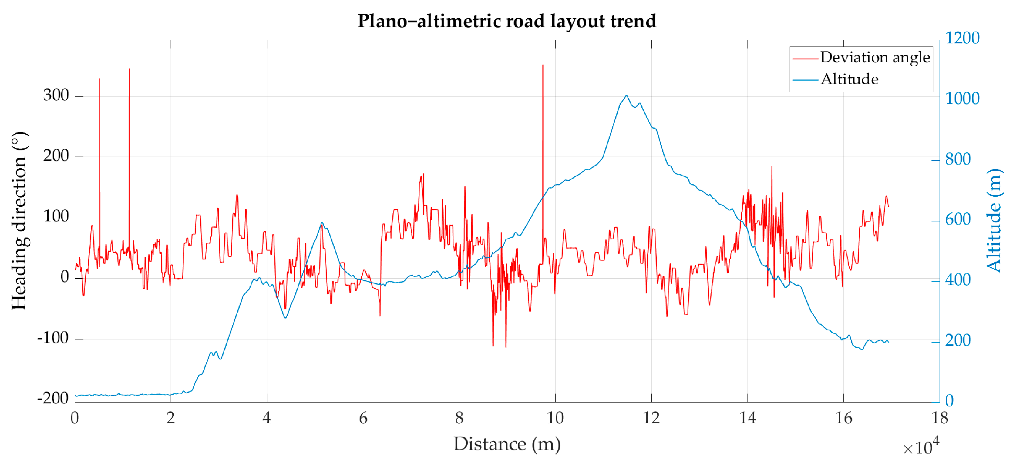
Once the azimuth (or heading angle) of each segment that composes the graph has been calculated, its trend and the elevations have been represented in a diagram as a function of the distance, as shown in Figure 7:
Subsequently, the Savitzky–Golay filter was applied to the heading angle trend for the purpose of smoothing the data, to increase their precision without distorting the signal tendency.
The results of this filtering process are shown in Figure 8, for the highway section used as an example, from the distance 40 km to the distance 55 km:
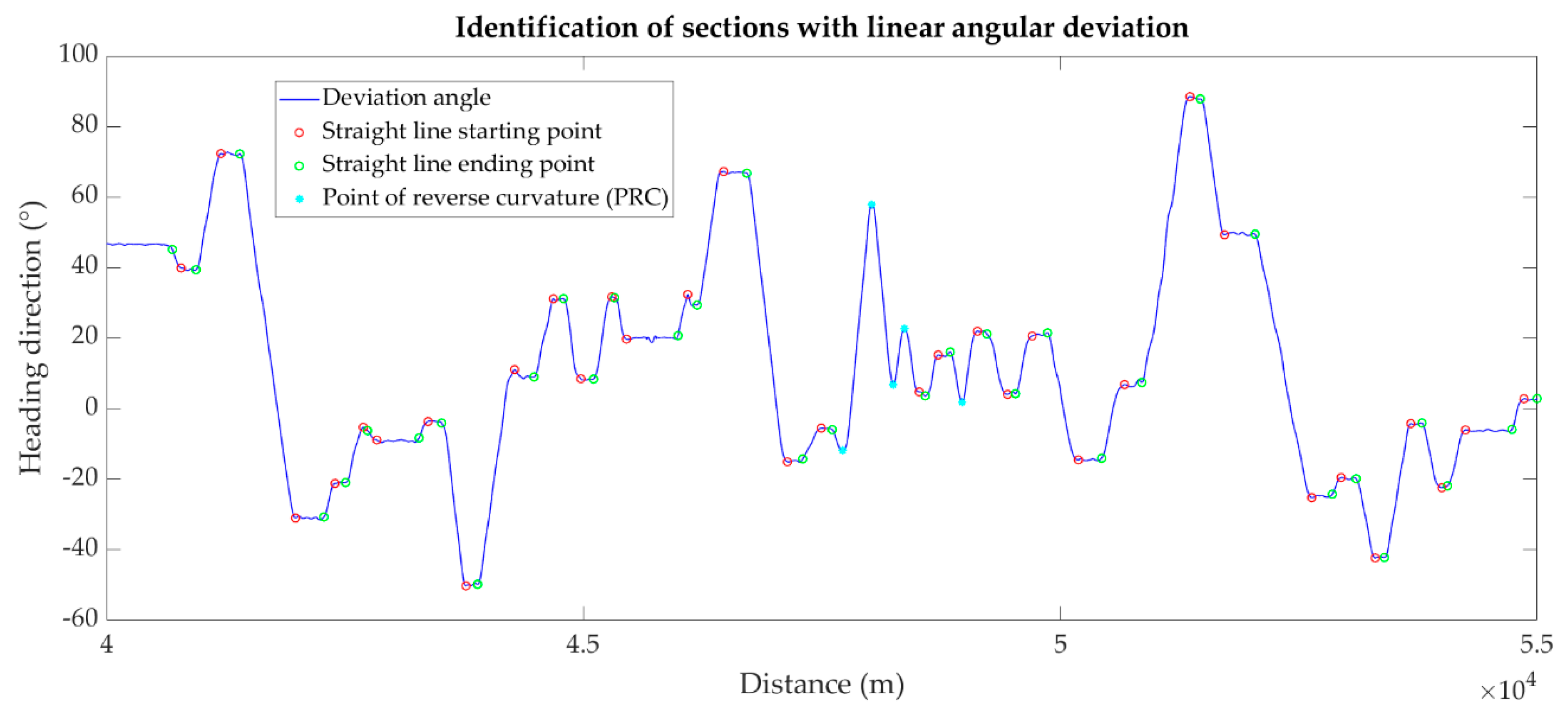
Subsequently, again by means of the programming code, a further method to determine the starting and ending points of the straight lines has been developed, through the analysis of the heading angle. A straight line has constant heading all the way along it, so in the distance–heading direction diagram, it is possible to identify in each plateau the elements with zero curvature. On the contrary, the circular arcs are represented by linear variations of the heading angle; conventionally, positive slope of the heading angle trend corresponds to right-handed curves; the negative slope corresponds to left-handed curves. When there are linear variations with a positive slope immediately followed by variations with a negative slope, or vice versa, in which no section with a zero slope is interposed, the points of reverse curvature can be identified at the vertices of the cusps.
Circular arcs with a length shorter than 45 m were excluded from the analysis, because they can be too short to carry out a reliable analysis, and the length may depend on excessive signal variations, not effectively smoothed by the application of the filter described above.
Figure 9 shows, between the distance 40 km and 55 km, the identification of the starting points of the straight lines in red, the ending points in green and the points of reverse curvature in cyan.
Once the coordinates of the starting and ending points of the straight sections have been identified, the starting and ending points of the circular arcs have also been defined, dividing each linear variations of the heading angle into five equal parts. The search of the geometric parameters of the elements—i.e., the radii and the coordinates of the centers of the arcs, the length of the straight lines—has been carried out by analyzing only the vertices falling in the central 3/5 of the different sections. The remaining areas—between the straight lines and the arcs or between two successive arcs—have a curved trend and have not been investigated due to the possible presence of transition curves inside the path (or in any case they can belong to the gaps where the trajectory of the vehicle used for the survey has made a progressive steering to enter the circular curve).
Once the vertices of the graph, corresponding to each geometric element, were known, the following features for the straight lines have been defined, as shown in Table 2: the length, the mean and the deviation of the azimuth, the starting and ending point in east and north coordinates.
The vertices of the graph that fall within the starting and ending points of a circular arcs were used to calculate the center and radius of each circumference, using a code that implements a least squares circle fitting algorithm. Table 3 shows the east and north coordinates of the center and the value of the radii of the circular arcs, the deviations, the east and north coordinates of the starting and ending points of each element, the lengths of the arcs and the values of the angles at the center:
The research findings consist of a procedure composed by three sequential phases, as described below.
3.1. Geometrizing Horizontal Alignment of an Existing Road Layout
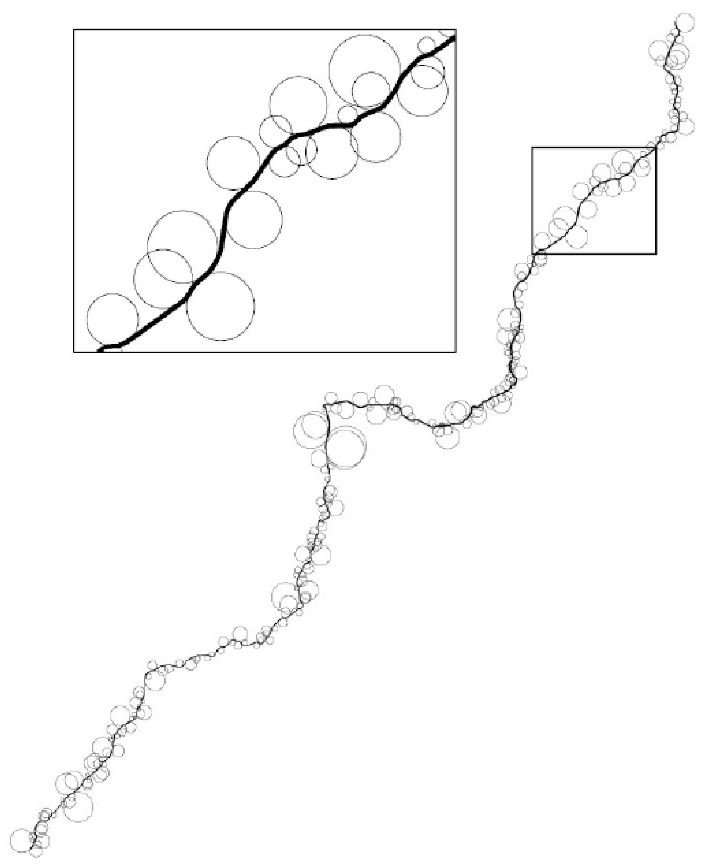
As shown in Figure 10, the Italian highway S.S. n. 4 has been completely geometrized by a succession of curves and straight lines; all the circumferences obtained by the previously described method, implemented in the original programming code, have been imported into the CAD (Computer-Aided Design) environment.
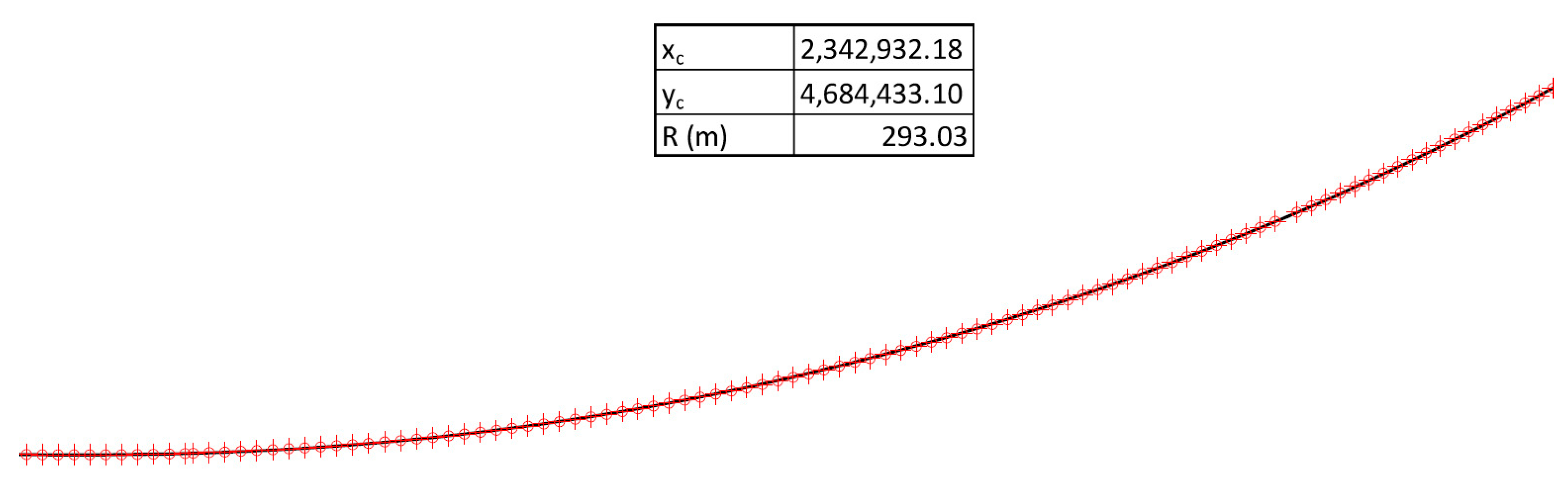
Figure 11 shows an example of a circumference computed by the circle fitting procedure implemented in the code, in which the points used for the least squares arc evaluation—and the center and radius coordinates definition obtained as a result—are represented in red (the curve obtained is in black):
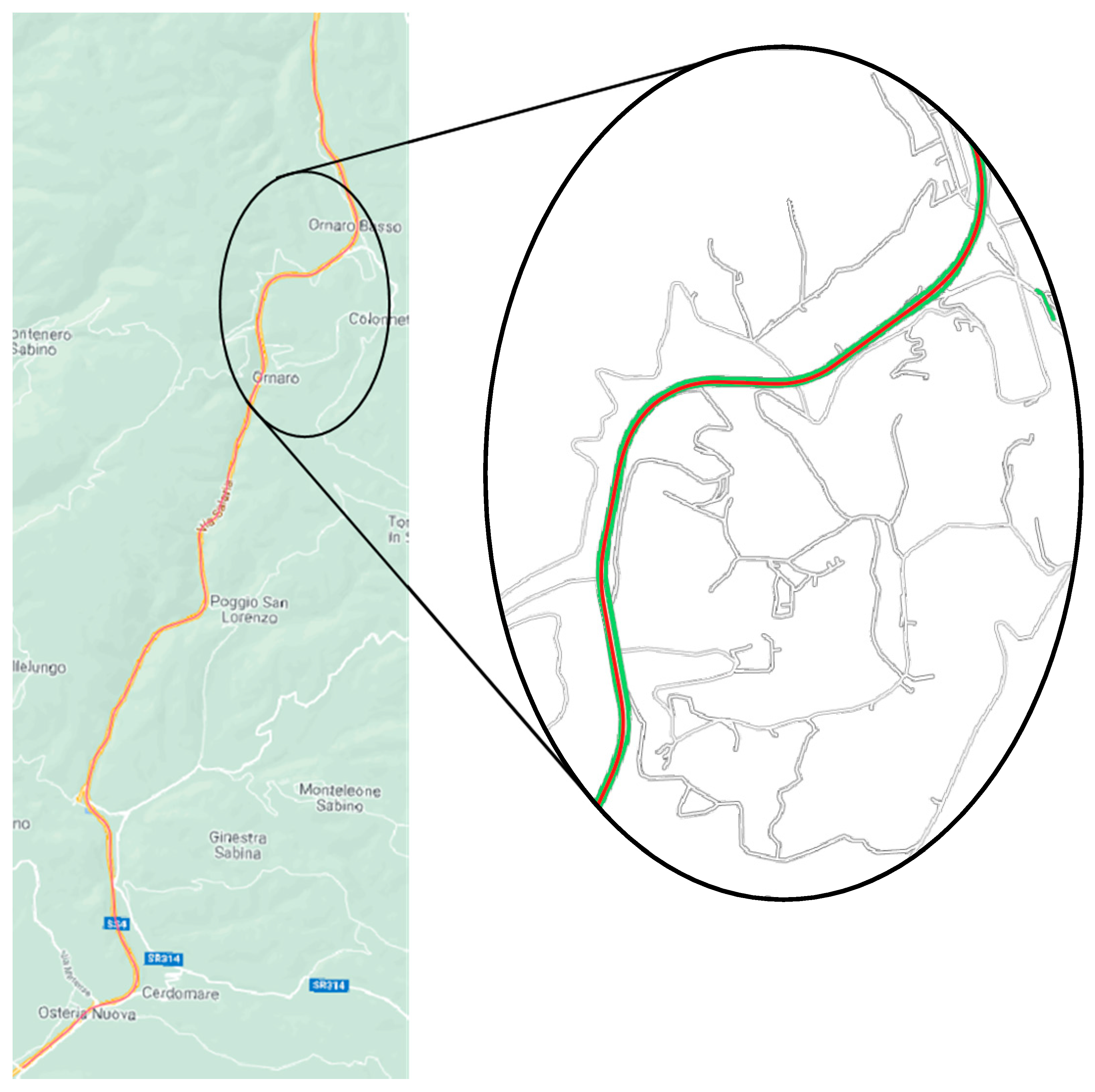
To test the accuracy of the results, after calculating the characteristic parameters of the circular arcs and the straight lines through the least square fitting, a qualitative comparison between the project axis obtained and the road layout, obtained from GIS basemaps, has been done. Even if it is not possible to consider Figure 12 as a quantitative validation, it can be noted that the two trends are overlapped in the entire distance considered.
3.2. Curvature Graph
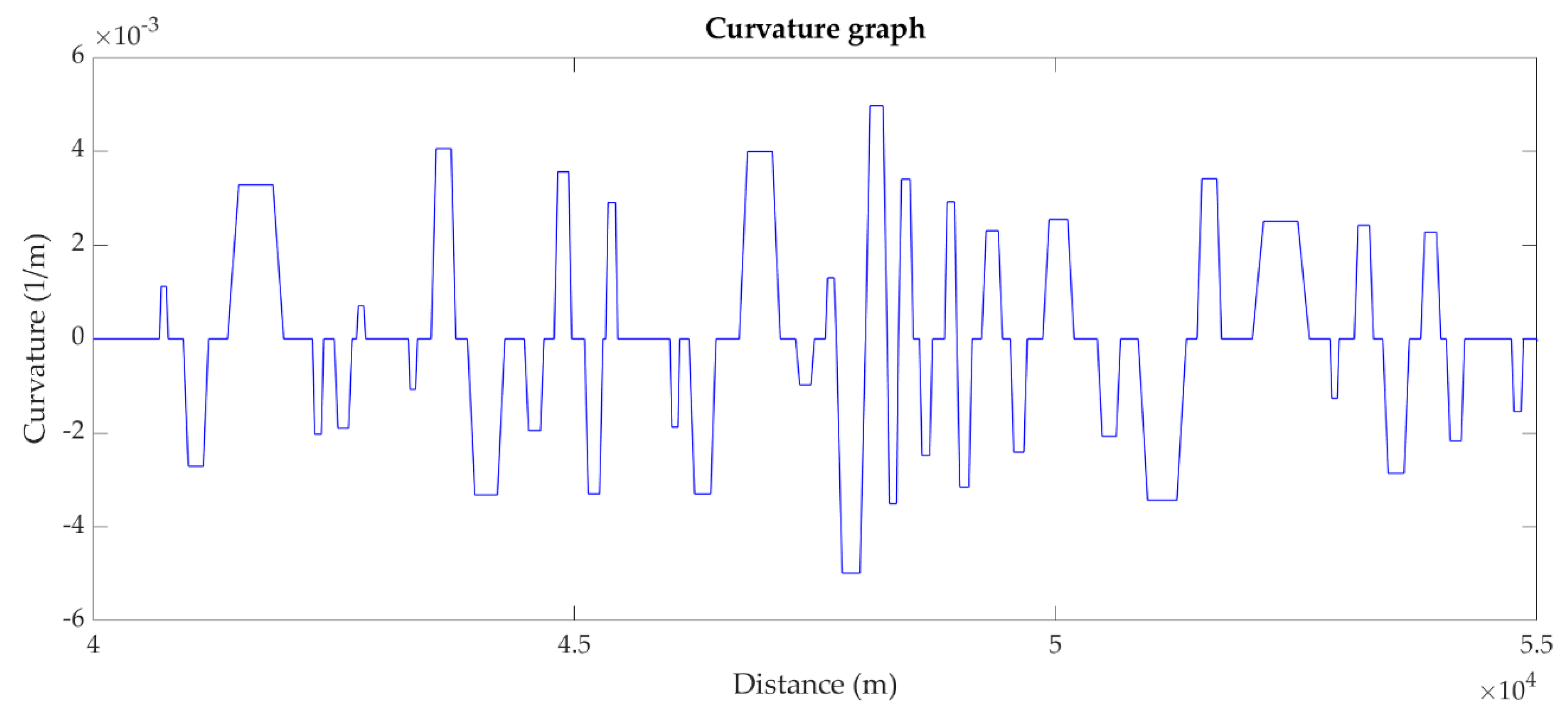
Once the calculation of the planimetric elements parameters has been completed, the curvature graph of the entire road layout has been subsequently constructed through another original code. Conventionally, the right-hand curves have been positioned above the reference (zero-curvature) line, assuming as positive the direction from point A to point B, while the left-hand curves have been positioned below. The transition zones, belonging neither to the straight lines nor to the circular arcs, have been treated as variable curvature elements, in order to connect elements having different curvatures.
Figure 13 shows the curvature graph for the segment taken as an example between the distance 40 km and 55 km:
3.3. Design Speed Profile
Once the curvature graph has been defined, an additional code has been implemented to calculate the design speed profile. The calculation follows the indications of the Italian Ministerial Decree 5 November 2001 [1] according to which:
The speed is constant all along the curve extension, and when the radius is less than a characteristic one (R2.5), it is determined by some graphs in the guidelines.
- On straight lines, on circular arcs with radius bigger than R2.5 and on clothoids, the design speed tends to the upper limit of the speed range; the acceleration spaces resulting from the exit from a circular curve and the deceleration spaces for the entrance to a curve are only limited to the elements considered.
- The acceleration and deceleration values are 0.8 m/s2.
- It is assumed that the longitudinal slopes do not influence the design speed.
The transition distance DT is the length in which the speed, according to the accepted theoretical model, passes from the value sd1 to sd2, of two consecutive elements. DT [m] is given by the following expression, where is the difference between sd1 and sd2 [km/h], is the average speed [km/h]:
The result of the calculation is shown in Figure 14:
After performing the described three sequential phases, a complete representation of the geometric elements composing the planimetric road layout, as well as the theoretical design speed trend along the alignment, is made available.
This kind of representation is useful when performing the safety analyses and, first of all, the ex post application of the regulatory model for the design verification. In this way, the procedure allows us to identify the sections where in-depth assessments have to be focused: if there are road sections in which some theoretical design conditions are not met significantly; in fact, further investigation should be conducted, especially when these sections also show other critical conditions related to safety or functional indicators (accident rates, heavy traffic conditions, black spots and so on).
As a general remark, the proposed assessments can be useful to pursue strategical and managing actions aimed at planning any road upgrading activities and at improving road safety performances.
4. Conclusions
The research carried out was aimed at implementing an automated, fast and economical procedure to identify the horizontal geometry of existing two-lane rural roads, based on the data obtained from the road graph of the network. In particular, it has been necessary to search for methods and algorithms capable of identifying the reference axes, such as in the design process of new tracks, which have to be mathematically described as simple and as continuous geometric elements (circular curves, clothoids and straight lines).
Using semi-automated procedures, implemented in a programming platform, the following main steps have been developed:
- Representation of the heading direction as a function of the distance, on the basis of the 3D spatial coordinates of the vertices of the road graph.
- Application of a Savitzky–Golay filter to the heading angle trend, with the purpose of smoothing the data and in order to identify straight line starting and ending points and points of reverse curvature.
- Analysis of the vertices falling within each element range and determination of the azimuth and length of the straight lines, of the radii and of the lengths of the circular arcs, by the application of a least square fitting procedure.
- Identification of the transition zones between the constant curvature elements (treated as clothoids) to compose a continuous curvature diagram.
- Once the curvature graph has been defined, calculation of the design speed profile by the implementation of an additional code.
The proposed method can be useful to analyze the technical characteristics of existing roads, especially in order to perform the ex post application of the regulatory models for the design verification. In particular, it allows us to perform road consistency analysis or to recognize other relevant effects in the road–user behavior interaction, such as the violation of:
- All these analyses are intended to assess Minimum and maximum lengths of each element with constant curvature, in relation to the drivers’ correct perception of the road layout.
- Correct succession of straight lines and circular arcs, or of two circular elements, in order to have gradual variations between their geometric characteristics.
- Optical, dynamic and road users’ comfort criteria of the variable curvature elements.
All these analyses are intended to assess the safety conditions for existing and open to traffic roads. In fact, considering the high accident rate found on the selected kind of roads, it is important to better study and understand the influence of the characteristics of the road on the users’ driving ability. Thus, the presented procedures are suitable for researchers to evaluate the effects of geometric inconsistencies on driver behaviors, as well as for practitioners (road administrators, technicians and professionals) to more easily develop the assessments on existing networks.
The effective contribution of this research to the state of practice is due to the opportunity to extract the track geometry from surveys or databases. The curvature graph and the design speed profile can be rapidly obtained, especially if the raw data are properly stored; the entire analysis process (starting from the data filtering to the final diagrams) can be uploaded and performed in a few hours. The short time needed is suitable for an extensive and systematic application of the methodology.
In fact, it will be possible to implement a code capable of quickly verifying the compliance of existing road layouts with the current design standards, in order to identify the sections that most differ from an optimal geometric configuration.
Author Contributions
Conceptualization, G.C. and G.D.S.; methodology, G.C.; software, G.D.S.; validation, G.C. and G.D.S.; formal analysis, G.C.; investigation, G.D.S.; data curation, G.C. and G.D.S.; writing—original draft preparation, G.D.S.; review and editing, G.C. and G.D.S.; supervision, G.C. All authors have read and agreed to the published version of the manuscript.
Funding
This research received no external funding.
Data Availability Statement
3rd Party Data.
Acknowledgments
We thank the national public company ANAS for making its graph available and for the technical support.
Conflicts of Interest
The authors declare no conflict of interest.
References
- IT Ministry for Infrastructures and Transport. Ministerial Decree Nov, 5-2001, No. 6792. Norme Funzionali e Geometriche per la Costruzione delle Strade; Official Gazette of IT Republic: Rome, Italy, 2002. [Google Scholar]
- IT Ministry for Infrastructures and Transport. Nuovo Codice della Strada. IT Law no. 285; Official Gazette of IT Republic: Rome, Italy, 1992. [Google Scholar]
- Cantisani, G.; Loprencipe, G. A statistics based approach for defining reference trajectories on road sections. Mod. Appl. Sci. 2013, 7, 32–46. [Google Scholar] [CrossRef]
- Anderson, I.; Bauer, K.M.; Collins, J.M.; Fitzpatrick, K.; Green, P.; Harwood, D.W.; Koppa, R.; Krammes, R.A.; Parma, K.D.; Poggioli, B.; et al. Alternative Design Consistency Rating Methods for Two-Lane Rural Highways; (No. FHWA-RD-99-172); United States Federal Highway Administration: Springfield, IL, USA, 2000.
- Ambros, J.; Valentova´, V. Identification of road horizontal alignment inconsistencies–A pilot study from the Czech Republic. Balt. J. Road Bridge Eng. 2016, 11, 62–69. [Google Scholar] [CrossRef]
- Weller, G.; Schlag, B.; Friedel, T.; Rammin, C. Behaviourally relevant road categorisation: A step towards self-explaining rural roads. Accid. Anal. Prev. 2008, 40, 1581–1588. [Google Scholar] [CrossRef]
- Gitelman, V.; Pesahov, F.; Carmel, R.; Bekhor, S. The identification of infrastructure characteristics influencing travel speeds on single-carriageway roads to promote selfexplaining roads. Transp. Res. Procedia 2016, 14, 4160–4169. [Google Scholar] [CrossRef] [Green Version]
- Edquist, J.; Rudin-Brown, C.M.; Lenne, M. Road Design Factors and Their Interactions with Speed and Speed Limits; Monash University Accident Research Centre—Report # 298; Monash University Accident Research Centre: Victoria, Australia, 2009; Volume 30, pp. 1–24. [Google Scholar]
- Scriabine, P. SEA Applied to Multimodal CorridorsMethodology Developed by France. The Case of the North Corridor; SETRA (Service d’Etudes Techniques des Routes et Autoroutes): Bagneux, France, 1999. [Google Scholar]
- Paysage Recueil D’expériences Paysage et Lisibilité—Approches Paysage et Sécurité Routière; SETRA (Service d’Etudes Techniques des Routes et Autoroutes): Bagneux, France, 2003.
- Cantisani, G.; Del Serrone, G.; Di Biagio, G. Calibration and validation of and results from a micro-simulation model to explore drivers’ actual use of acceleration lanes. Simul. Model. Pract. Theory 2018, 89, 82–99. [Google Scholar] [CrossRef]
- Abele, L.; Møller, M. The relationship between road design and driving behavior. In Proceedings of the RSS 2011: Road Safety and Simulation 2011 Conference, Indianapolis, IN, USA, 14–16 September 2011. [Google Scholar]
- Ambunda, R.; Sinclair, M. Effect of two-lane two-way rural roadway design elements on road safety. Int. J. Innov. Technol. Explor. Eng. 2019, 8, 632–637. [Google Scholar]
- De Jager, T.M. Investigating Dangerous Overtaking Manoeuvres: The Effect of Road Design Elements on the Psychological State of Drivers. Ph.D. Thesis, Stellenbosch University, Stellenbosch, South Africa, 2019. [Google Scholar]
- Hisham, M.A.M.N.; Adnan, A.; Umar, R.Z.R.; Samuel, S.; Hanafi, M.; Ani, M.H. Effect of road design on hazard anticipation behavior among motorcyclists during merging in traffic. Hum. Factors Ergon. J. 2019, 4, 92–98. [Google Scholar]
- Li, Z.; Chitturi, M.V.; Bill, A.R.; Noyce, D.A. Automated identification and extraction of horizontal curve information from geographic information system roadway maps. Transp. Res. Rec. 2012, 2291, 80–92. [Google Scholar] [CrossRef] [Green Version]
- Watters, P.; O’Mahony, M. The relationship between geometric design consistency and safety on rural single carriageways in Ireland. In Proceedings of the European Transport Conference, Leiden, The Netherlands, 17–19 October 2007. [Google Scholar]
- Andrášik, R.; Bíl, M. Efficient road geometry identification from digital vector data. J. Geogr. Syst. 2016, 18, 249–264. [Google Scholar] [CrossRef]
- Di Mascio, P.; Di Vito, M.; Loprencipe, G.; Ragnoli, A. Analisi di sensibilità dei metodi di calcolo per la determinazione della geometria stradale. In Proceedings of the XXVI National PIARC Conference—Tema Strategico D-Qualità delle infrastrutture stradali, Rome, Italy, 27–30 October 2010; ISBN 978-88-905397-0-1. (In Italian). [Google Scholar]
- Luo, W.; Li, L.; Wang, K.C. Automated pavement horizontal curve measurement methods based on inertial measurement unit and 3D profiling data. J. Traffic Transp. Eng. 2016, 3, 137–145. [Google Scholar] [CrossRef] [Green Version]
- Marinelli, G.; Bassani, M.; Piras, M.; Lingua, A. Mobile mapping systems and spatial data collection strategies assessment in the identification of horizontal alignment of highways. Transp. Res. Part C Emerg. Technol. 2017, 79, 257–273. [Google Scholar] [CrossRef] [Green Version]
- Puente, I.; Gonz´alez-Jorge, H.; Mart´ınez-Sa´nchez, J.; Arias, P. Review of mobile mapping and surveying technologies. Measurement 2013, 46, 2127–2145. [Google Scholar] [CrossRef]
- Wang, K.; Hou, Z.; Gong, W. Automation techniques for Digital Highway Data Vehicle (DHDV). In Proceedings of the 7th International Conference on Managing Pavement Assets, Calgary, AB, Canada, 23–28 June 2008. [Google Scholar]
- Gavil´an, M.; Balcones, D.; Marcos, O.; Llorca, D.F.; Sotelo, M.A.; Parra, I.; Ocan˜a, M.; Aliseda, P.; Yarza, P.; Am´ırola, A. Adaptive road crack detection system by pavement classification. Sensors 2011, 11, 9628–9657. [Google Scholar] [CrossRef] [PubMed]
- Specht, C.; Wilk, A.; Koc, W.; Karwowski, K.; Dąbrowski, P.; Specht, M.; Grulkowski, S.; Chrostowski, P.; Szmagliński, J.; Czaplewski, K.; et al. Verification of GNSS measurements of the railway track using standard techniques for determining coordinates. Remote Sens. 2020, 12, 2874. [Google Scholar] [CrossRef]
- Koc, W.; Specht, C.; Szmaglinski, J.; Chrostowski, P. A method for determination and compensation of a cant influence in a track centerline identification using GNSS methods and inertial measurement. Appl. Sci. 2019, 9, 4347. [Google Scholar] [CrossRef] [Green Version]
- Dąbrowski, P.S.; Specht, C.; Koc, W.; Wilk, A.; Czaplewski, K.; Karwowski, K.; Specht, M.; Chrostowski, P.; Szmagliński, J.; Grulkowski, S. Installation of GNSS receivers on a mobile railway platform–methodology and measurement aspects. Zesz. Nauk. Akad. Mor. Szczec. 2019, 60, 18–26. [Google Scholar]
- Ai, C.; Tsai, Y. Automatic horizontal curve identification and measurement method using GPS data. J. Transp. Eng. 2015, 141, 04014078. [Google Scholar] [CrossRef] [Green Version]
- Castro, M.; Iglesias, L.; Rodr´ıguez-Solano, R.; Sa´nchez, J.A. Geometric modelling of highways using global positioning system (GPS) data and spline approximation. Transp. Res. Part C Emerg. Technol. 2006, 14, 233–243. [Google Scholar] [CrossRef]
- Ben-Arieh, D.; Chang, S.; Rys, M.; Zhang, G. Geometric modeling of highways using global positioning system data and B-spline approximation. J. Transp. Eng. 2004, 130, 632–636. [Google Scholar] [CrossRef]
- Di Mascio, P.; Di Vito, M.; Loprencipe, G.; Ragnoli, A. Procedure to determine the geometry of road alignment using GPS data. Procedia Soc. Behav. Sci. 2012, 53, 1202–1215. [Google Scholar] [CrossRef] [Green Version]
- Crisman, B.; Robba, A. Safety Evaluation: Practical Use of Collected Data Vehicle to Obtain Geometric Information of Existing Roadway; Società Italiana Infrastrutture Viarie SIIV: Catania, Italy, 2005; volume 400, pp. 1–21. [Google Scholar]
- Zhang, S.; Won, M.; Son, S.H. Low-cost realtime horizontal curve detection using inertial sensors of a smartphone. In Proceedings of the 2016 IEEE 84th Vehicular Technology Conference (VTC-Fall), Montréal, QC, Canada, 18–21 September 2016; pp. 1–5. [Google Scholar]
- Kåsa, I. A circle fitting procedure and its error analysis. IEEE Trans. Instrum. Meas. 1976, 25, 8–14. [Google Scholar] [CrossRef]
- Ciroi, S. I Minimi Quadrati. Chapter 11. pp. 123–138. Available online: http://dipastro.pd.astro.it/ciroi/espfis1/esperI_cap11.pdf (accessed on 9 November 2020).
- Maisonobe, L. Finding the Circle that Best Fits a Set of Points. 2007. Available online: http://www.spaceroots.org/documents/circle/circle-fitting.pdf (accessed on 9 November 2020).
- Bassani, M.; Marinelli, G.; Piras, M. Identification of horizontal circular arc from spatial data sources. J. Surv. Eng. 2016, 142, 04016013. [Google Scholar] [CrossRef] [Green Version]
- Gander, W.; Golub, G.H.; Strebel, R. Least-squares fitting of circles and ellipses. BIT Numer. Math. 1994, 34, 558–578. [Google Scholar] [CrossRef]
- Luo, W.; Li, L.; Wang, K.C. Automatic horizontal curve identification and measurement using mobile mapping system. J. Surv. Eng. 2018, 144, 04018007. [Google Scholar] [CrossRef]
- Walton, D.J.; Meek, D.S. A controlled clothoid spline. Comput. Graph. 2005, 29, 353–363. [Google Scholar] [CrossRef]
- Cantisani, G.; Dondi, D.; Loprencipe, G.; Ranzo, A. Spline curves for geometric modeling of highway design. In Proceedings of the II International Congress SIIV—New Technologies and Modeling Tools for Roads, Firenze, Italy, 27–29 October 2004. [Google Scholar]
- Savitzky, A.; Golay, M.J.E. Smoothing and differentiation of data by simplified least squares procedures. Anal. Chem. 1964, 36, 1627–1639. [Google Scholar] [CrossRef]
- Garach, L.; De Oña, J.; Pasadas, M. Determination of alignments in existing roads by using spline techniques. Math. Comput. Simul. 2014, 102, 144–152. [Google Scholar] [CrossRef]
- Li, W.; Pu, H.; Schonfeld, P.; Song, Z.; Zhang, H.; Wang, L.; Wang, J.; Peng, X.; Peng, L. A method for automatically recreating the horizontal alignment geometry of existing railways. Comput. Aided Civ. Infrastruct. Eng. 2019, 34, 71–94. [Google Scholar] [CrossRef] [Green Version]
- Gikas, V.; Stratakos, J. A novel geodetic engineering method for accurate and automated road/railway centerline geometry extraction based on the bearing diagram and fractal behavior. IEEE Trans. Intell. Transp. Syst. 2011, 13, 115–126. [Google Scholar] [CrossRef]
- Coope, I.D. Circle fitting by linear and nonlinear least squares. J. Optim. Theory Appl. 1993, 76, 381–388. [Google Scholar] [CrossRef] [Green Version]
- Garach, L.; de Oña, J.; Pasadas, M. Mathematical formulation and preliminary testing of a spline approximation algorithm for the extraction of road alignments. Autom. Constr. 2014, 47, 1–9. [Google Scholar] [CrossRef]
Figure 1.
A least square circle fitting example.

Figure 2.
Road accidents, deaths and injuries for different road categories. Source: Italian National Institute of Statistics—Istat (2018).
Figure 2.
Road accidents, deaths and injuries for different road categories. Source: Italian National Institute of Statistics—Istat (2018).

Figure 3.
Geographical representation of the road network managed by ANAS S.p.A. as of 10 October 2019.
Figure 3.
Geographical representation of the road network managed by ANAS S.p.A. as of 10 October 2019.

Figure 4.
Example of a smoothing technique obtained by applying a low-pass filter.

Figure 5.
Graph of the HWY 4 from A to B.

Figure 6.
Example of Azimuth: heading angle from the magnetic north.

Figure 7.
Heading direction and elevation trends along the HWY 4.

Figure 8.
Heading direction graph, compared to moving average filter ‘sgolayfilt’ type of the HWY 4—from the distance 40 km to the distance 55 km.
Figure 8.
Heading direction graph, compared to moving average filter ‘sgolayfilt’ type of the HWY 4—from the distance 40 km to the distance 55 km.

Figure 9.
Identification of straight line starting and ending points and points of reverse curvature of the HWY 4—from the distance 40 km to the distance 55 km.
Figure 9.
Identification of straight line starting and ending points and points of reverse curvature of the HWY 4—from the distance 40 km to the distance 55 km.

Figure 10.
Circumferences obtained by fitting the circular arcs of the road.

Figure 11.
Least square circle fitting for the center and radius coordinates definition.

Figure 12.
A qualitative comparison between the calculated project axis and the road layout got from a GIS basemap and a zoom of the HWY 4—from the distance 40 km to the distance 55 km.
Figure 12.
A qualitative comparison between the calculated project axis and the road layout got from a GIS basemap and a zoom of the HWY 4—from the distance 40 km to the distance 55 km.

Figure 13.
Curvature graph of the HWY 4—from the distance 40 km to the distance 55 km.

Figure 14.
Design speed profile of the HWY 4—from the distance 40 km to the distance 55 km.


Table 1.
Information related to each vertex of the graph.
| E | N | Q | i | Azimuth | m | q | Partial Length | Distance |
|---|---|---|---|---|---|---|---|---|
| (m) | (m) | (m) | (°) | y = mx + q | (m) | (m) | ||
| 790,885.2 | 4,654,322.3 | 24.79 | 1 | 22.8 | 2.4 | 2,769,909.0 | 1.286 | 0.00 |
| 790,885.7 | 4,654,323.4 | 24.776 | 2 | 22.6 | 2.4 | 2,749,917.0 | 1.289 | 1.29 |
| 790,886.2 | 4,654,324.6 | 24.763 | 3 | 22.4 | 2.4 | 2,738,193.8 | 1.290 | 2.57 |
| 790,886.7 | 4,654,325.8 | 24.756 | 4 | 22.5 | 2.4 | 2,740,488.4 | 1.289 | 3.86 |
| 790,887.2 | 4,654,327.0 | 24.737 | 5 | 22.3 | 2.4 | 2,723,133.1 | 1.292 | 5.15 |
| 790,887.7 | 4,654,328.2 | 24.723 | 6 | 21.9 | 2.5 | 2,686,229.1 | 1.294 | 6.44 |
| 790,888.2 | 4,654,329.4 | 24.726 | 7 | 21.8 | 2.5 | 2,672,991.9 | 1.295 | 7.74 |
| 790,888.7 | 4,654,330.6 | 24.712 | 8 | 21.5 | 2.5 | 2,648,700.0 | 1.300 | 9.03 |
| 790,889.1 | 4,654,331.8 | 24.697 | 9 | 21.3 | 2.6 | 2,626,662.2 | 1.305 | 10.33 |
| 790,889.6 | 4,654,333.0 | 24.692 | 10 | 21.1 | 2.6 | 2,608,805.8 | 1.306 | 11.64 |
Table 2.
Information related to straight lines.
| L | α | σ | Es | Ns | Ee | Ne | |
|---|---|---|---|---|---|---|---|
| (m) | (°) | (m) | (m) | (m) | (m) | (m) | |
| S.L. 1 | 205.52 | 19.17 | 0.58 | 2,313,937.5 | 4,651,583.2 | 2,313,870.0 | 4,651,389.1 |
| S.L. 2 | 68.64 | 25.65 | 0.59 | 2,313,998.1 | 4,651,718.7 | 2,313,968.6 | 4,651,656.8 |
| S.L. 3 | 79.56 | 27.58 | 0.53 | 2,314,072.8 | 4,651,861.9 | 2,314,036.0 | 4,651,791.4 |
| S.L. 4 | 259.91 | 23.39 | 0.38 | 2,314,209.1 | 4,652,169.7 | 2,314,105.9 | 4,651,931.2 |
| S.L. 5 | 20.36 | 38.45 | 0.09 | 2,314,311.8 | 4,652,333.7 | 2,314,299.1 | 4,652,317.8 |
| S.L. 6 | 105.43 | 15.86 | 0.44 | 2,314,403.7 | 4,652,552.1 | 2,314,374.9 | 4,652,450.7 |
| S.L. 7 | 12.95 | 22.07 | 0.01 | 2,314,448.1 | 4,652,676.4 | 2,314,443.3 | 4,652,664.4 |
| S.L. 8 | 119.66 | −24.32 | 0.20 | 2,314,382.7 | 4,653,143.4 | 2,314,432.0 | 4,653,034.3 |
| S.L. 9 | 340.07 | 18.06 | 0.85 | 2,314,476.8 | 4,653,938.4 | 2,314,371.3 | 4,653,615.2 |
| S.L. 10 | 218.78 | 91.24 | 0.24 | 2,315,295.8 | 4,654,341.2 | 2,315,077.1 | 4,654,345.9 |
Table 3.
Information related to circular arcs.
| Ec | Nc | R | σ | Es | Ns | Ee | Ne | L | α | |
|---|---|---|---|---|---|---|---|---|---|---|
| (m) | (m) | (m) | (m) | (m) | (m) | (m) | (m) | (m) | (rad) | |
| C.A. 1 | 2,314,485.9 | 4,651,399.3 | 578.3 | 0.04 | 2,313,943.0 | 4,651,598.5 | 2,313,961.1 | 4,651,642.2, | 47.30 | 0.08 |
| C.A. 2 | 2,313,038.2 | 4,652,397.5 | 1165 | 0.10 | 2,314,079.7 | 4,651,875.5 | 2,314,099.2 | 4,651,916.5 | 45.39 | 0.04 |
| C.A. 3 | 2,314,581.2 | 4,652,045.8 | 389.5 | 0.26 | 2,314,223.7 | 4,652,201.1 | 2,314,278.3 | 4,652,290.9 | 105.34 | 0.27 |
| C.A. 4 | 2,314,143.7 | 4,652,503.7 | 236.6 | 0.39 | 2,314,330.1 | 4,652,357.9 | 2,314,367.8 | 4,652,427.3 | 79.33 | 0.34 |
| C.A. 5 | 2,315,098.3 | 4,652,369.9 | 717.6 | 0.15 | 2,314,411.2 | 4,652,577.3 | 2,314,435.5 | 4,652,644.9 | 71.88 | 0.10 |
| C.A. 6 | 2,314,120.3 | 4,652,837.3 | 364.3 | 0.25 | 2,314,473.0 | 4,652,746.9 | 2,314,460.6 | 4,652,967.5 | 224.53 | 0.62 |
| C.A. 7 | 2,314,926.2 | 4,653,387.6 | 596.8 | 0.33 | 2,314,349.3 | 4,653,235.8 | 2,314,345.5 | 4,653,526.4 | 293.57 | 0.49 |
| C.A. 8 | 2,315,049.6 | 4,653,733.4 | 611.5 | 0.81 | 2,314,547.7 | 4,654,083.5 | 2,314,923.2 | 4,654,331.0 | 460.79 | 0.75 |
Publisher’s Note: MDPI stays neutral with regard to jurisdictional claims in published maps and institutional affiliations. |
© 2020 by the authors. Licensee MDPI, Basel, Switzerland. This article is an open access article distributed under the terms and conditions of the Creative Commons Attribution (CC BY) license (http://creativecommons.org/licenses/by/4.0/).
Share and Cite
MDPI and ACS Style
Cantisani, G.; Del Serrone, G. Procedure for the Identification of Existing Roads Alignment from Georeferenced Points Database. Infrastructures 2021, 6, 2. https://0-doi-org.brum.beds.ac.uk/10.3390/infrastructures6010002
AMA Style
Cantisani G, Del Serrone G. Procedure for the Identification of Existing Roads Alignment from Georeferenced Points Database. Infrastructures. 2021; 6(1):2. https://0-doi-org.brum.beds.ac.uk/10.3390/infrastructures6010002
Chicago/Turabian StyleCantisani, Giuseppe, and Giulia Del Serrone. 2021. "Procedure for the Identification of Existing Roads Alignment from Georeferenced Points Database" Infrastructures 6, no. 1: 2. https://0-doi-org.brum.beds.ac.uk/10.3390/infrastructures6010002