Uncertainty in Building Inspection and Diagnosis: A Probabilistic Model Quantification

Abstract

In the field of building inspection and diagnosis, uncertainty is common and surveyors are aware of it, although it is not easily measured. This research proposes a model to quantify uncertainty based on the inspection of rendered façades. A Bayesian network is developed, considering three levels of variables: characteristics of the building, façade and exposure conditions; causes of defects; and defects. To compute conditional probabilities, the results of an inspection campaign from the literature are used. Then, the proposed model is validated and verified using inspection results from another sample, the combination of a strength-of-influence diagram and sensitivity analysis and the application of the model to a case study. Results show that the probabilities computed by the model are a reasonable representation of the hesitancy in decision making during the diagnosis process based only on visual observation. For instance, design and execution errors show lower probabilities due to not being verifiable a posteriori without detailed documentation. The proposed model may be extended and replicated for other building materials in the future, as it may be a useful tool to improve the perception of uncertainty in a key stage of building maintenance or rehabilitation.

1. Introduction

1.1. Background, Problem and Purpose

Physical degradation is one of the processes that may result in the obsolescence of buildings, as some performance requirements stop being fulfilled and, eventually, the building or its elements reach the end of their service life. Physical, chemical and mechanical degradation agents gradually affect building elements and, together with natural ageing, lead to deterioration [1]. This general issue requires action to extend the buildings’ service life, such as carrying out maintenance activities to hinder the degradation mechanisms.

In the context of maintenance planning, which combines different maintenance strategies (reactive or proactive, whether preventive or condition based [2]), building inspections provide valuable data on the degradation condition of the building elements, informing stakeholders and helping them to make better decisions.

Nevertheless, uncertainty is associated with the inspection and diagnosis activities performed to assess the degradation state of buildings and their elements. Even though this uncertainty is rarely quantified, surveyors, designers, engineers and prescribers are aware of some level of subjectivity inherent to all diagnoses, as well as of the vulnerability and unpredictability of outcomes stemming from recommendations and decisions. Additionally, the levels of uncertainty vary according to several contextual factors.

During inspection and diagnosis operations, uncertainty may arise at different stages, namely [3]:

• During the observation, understanding and analysis of degradation phenomena, depending on:
  • The knowledge and experience of the surveyor
  • The circumstances of observation (for instance, means of access or weather conditions)
  • The availability and effective use of expeditious means of observation (more relevant when the signs of failure are invisible to the naked eye)
  • The preliminary planning of the on-site inspection (for instance, consulting available documents about the building)
• During the process of clearly identifying the defect, its causes and the best course of action to reinstate performance levels that fulfil the building element’s functional requirements, while making decisions involving:
  • The determination of the need of additional in situ diagnosis methods or laboratory tests
  • The choice of in situ diagnosis methods or laboratory tests, if needed, considering their contribution for a more accurate diagnosis (usefulness, intrusiveness, ease of execution, precision, type of results, cost, time needed to obtain results)
  • The decision about whether eventual results of in situ diagnosis methods or laboratory tests are conclusive and enough [4]
  • The identification of the defect and its causes based on all available data (information about the building, visual inspection and any additional diagnosis method)
  • The development of recommendations according to the diagnosis.
• During the communication of recommendations in a non-ambiguous and detailed way, allowing stakeholders to weigh several parameters that may affect decision making

Uncertainty is associated with risk, and the former needs to be acknowledged so that any danger is not completely unexpected. Risks may be associated with, among others [3], (i) an incorrect diagnosis, causing resources to be allocated towards activities that end up not extending durability; (ii) an inadequate application of repair techniques, although resulting from a correct diagnosis; (iii) a decontextualised evaluation of the built object, eventually disregarding occasional historical value; and (iv) an incorrect safety assessment of the building, leading to human and material losses.

To overcome the blurred perception of uncertainty by surveyors during the process of diagnosis of the degradation, it is necessary to find a way to clarify that perception. Quantification measures are expected to be more effective in promoting that clarification process.

This research intends to propose a model of quantification of uncertainty in building inspection and diagnosis. With that purpose in mind, the scope of building inspection and diagnosis was limited to a type of façade cladding (façade renders) so that the problem could be outlined in a simpler manner. Additionally, the diagnosis of a detected defect was analysed to define the factors that influence it (e.g., causes). Furthermore, those factors had to be adapted to a quantification model. It is expected that the findings of this research will help surveyors in enhancing their understanding of the underlying uncertainty associated with the diagnosis process, thus improving it.

In this paper, after a brief description of the issue at hand, Bayes’ theorem and Bayesian networks are outlined. Then, the materials and methods used in this study are described, including not only those needed to create the proposed model but also those to assess it. Next, the results are presented in terms of the development of the model and respective validation and verification. Results are then discussed, and the main conclusions are drawn.

1.2. Formulations of Uncertainty

There is a large range of disciplines that refer to uncertainty, whether applying concepts of decision theory, statistics or other quantification fields. In this section, the methods of Bayes’ theorem and Bayesian networks to deal with uncertainty are highlighted.

1.2.1. Bayes’ Theorem

The diagnosis process in the context of building inspection involves making decisions that can be compared to those in the medical (clinical) context, with the necessary adaptations. In differential diagnosis, uncertainty can be faced complementing the competing-hypotheses heuristic with Bayesian probability [5]. In that context, uncertainty may be associated with [5] (i) clinical information, (ii) interpretation of laboratory data, (iii) the connection between clinical findings and diseases and (iv) the effects of different therapies. These items can be matched with parameters involved in building diagnosis, namely (i) information about the building and its components, (ii) interpretation of data from in situ or laboratory tests, (iii) the connection between defects and their causes and (iv) the effects of different repair techniques.

The same way the mathematical form of Bayes’ theorem can be used in a clinical context when estimates of the likelihood of a disease for relevant groups are available [5], it can also be applied in building diagnosis when estimates of the likelihood of causes of defects are employable for relevant groups of building elements or materials. Nevertheless, even without calculations, the formulation of Bayes’ theorem can help clinicians and surveyors to address decisions about the possible relevance of additional information [5].

Although Bayes’ theorem may have limitations, its logic may be useful to improve systematic problem solving during a diagnosis process. Bayes’ theorem’s simplest form is presented in Equation (1):

P (cause | defects) = [P (defects | cause) × P (cause)]/P (defects)

(1)

representing the probability P of a building element or material being subjected to a cause of defect, given the observation of a set of defects. In Equation (1), the numerator refers to the product between (i) the probability of having that set of defects, given the presence of the considered cause, and (ii) the probability of having the cause in the population of building elements and materials. That population may refer to specific characteristics, such as elements only in the building envelope or only cementitious materials. The numerator is divided by the probability of occurrence of the set of defects [3].

The limitations of using Bayes’ theorem are associated with [5] requiring large datasets, the shifting availability of probability estimates (variations of available data according to symptoms and diseases), the complexity of stating hypotheses based on anomalous manifestations and the difficulty of computing probabilities from memory. Moreover, Bayes’ theorem does not conciliate the hypothesis of multiple diseases occurring in the same case (or multiple causes in the same element), nor the non-independence of symptoms associated with a single disease (or defects and a single cause).

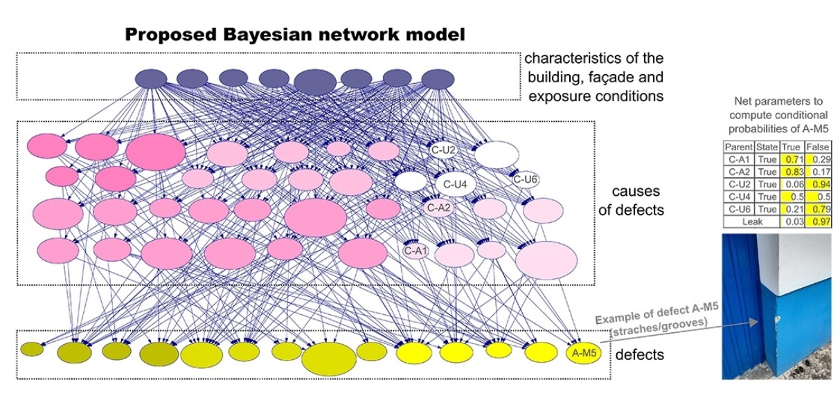
1.2.2. Bayesian Networks

To deconstruct the analysis of elaborate problems, their components can be reduced to a finite number of states. An option is to formulate binary hypotheses, modelling numerous scenarios, which may still be incomplete, as the systems’ components often require the assumption of multi-states. In these cases, Boolean or classic logic may be insufficient [6]. Such probabilistic events can be framed within Bayesian networks, which provide a theoretical context to represent events using discrete random variables [7]. The relationship between those events is then represented by conditional probabilities [6].

Considering these premises, the degradation mechanisms of a building can be represented as a system and analysed, breaking down its components. Thus, a Bayesian network (BN) can be developed, where uncertainty would be represented by the conditional probability tables (CPTs) associated with each variable. In the present research, the system was delimited to rendered façades, as part of a more complex system. In this way, a lower number of variables may be considered to explore the applicability of the methodology.

In a BN, variables are represented by nodes and the relationship between nodes is represented by arcs. Those arcs are unidirectional, denoting the influence of one node (at the tail of the arc) in another node (at the head of the arc). That graphical structure is complemented by the numerical properties of each node, which are encoded in CPTs, prepared according to the influence of prior nodes [8].

In the field of building performance, a BN has already been developed to predict the condition of buildings in order to assist maintenance planning [9,10,11]. Other authors [12,13] proposed the use of dynamic Bayesian networks to model the deterioration process of structural systems as a method suitable to plan and optimise monitoring activities, as well as inspection and other maintenance actions of such systems. Bayesian belief networks were also used, for instance, to assess the probability of collapse of structures associated with the corrosion of reinforcement in concrete structures of buildings, for repair optimisation [14] and to monitor the condition state of a bridge [15]. Additionally, maintenance scenarios were also explored using Bayesian networks to support decision making at the design stage of a building, accommodating a design-for-maintainability approach [16,17]. Most of the mentioned research in the literature input conditional probabilities in the BN based on the judgement of experts, while the model proposed in this research is based on an existing dataset from on-site inspections, providing conditional probabilities from real scenarios. Additionally, the proposed model deals with a specific problem that has not been focused on previous research about uncertainty—the inspection and diagnosis of non-structural materials of the building envelope. Thus, the present research adds novelty to the literature.

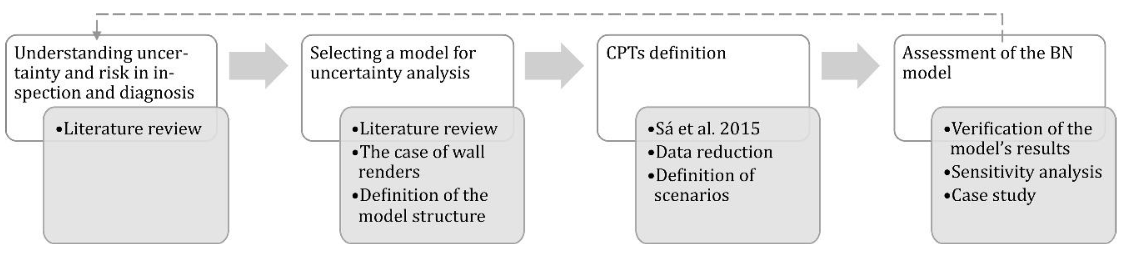
2. Materials and Methods

This study adopted an observational research methodology to create a model to quantify uncertainty in building inspection and diagnosis. Developing such a model required a set of analysis, execution and verification steps. Research procedures included (Figure 1) understanding uncertainty and risk in the studied context, selecting a model to perform uncertainty analysis, defining CPTs and assessing the BN model. Within these procedures, several research steps were performed, including selecting a dataset (from the literature) and analysing quantitative information.

At an initial stage, a search for common and accessible BN modelling tools was performed, considering the capabilities of each software and the objectives of the research. GeNIe Modeler [18] was chosen due to the reliability of data analysis, its user-friendly interface and its availability for academic users.

Based on the sample of Sá et al. [19], the model refers to existing rendered façades in urban buildings (with residential, office and commercial uses). The sample includes 99 different façades from the inspection of 52 buildings, all located in the metropolitan area of Lisbon, Portugal. The inspections occurred in 2010 [19]. The buildings were totally or partially occupied and were associated with different types of actors, such as owners and tenants. Inspections were solely based on visual observation and small interviews with owners or tenants.

2.1. Development of the Model and Defining CPTs

The sample points correspond to defects visually detected on each inspected façade. Each observation included information about (i) the building (age, exposure to aggressive agents—rain–wind action, humidity, pollution); (ii) the façade (orientation, type of render, execution method and finish, type of washes and washing frequency) it was detected on; and (iii) information about the probable causes inferred during the diagnosis. Data about the number of floors of the building, type of façade (front, since, rear), area of the rendered surface, proximity to heat sources, inclusion of a reinforcement mesh, contact with people and animals, and recommended diagnosis methods and repair techniques were also available but were excluded from the analysis. Only the most influential characteristics of the building and façades for their degradation were considered, according to whether they seemed likely to affect defect occurrence [20], while diagnosis methods and repair techniques were not considered a part of the cause–effect relationship represented in the proposed model.

Thus, the relevant variables for the analysis of the degradation of rendered façades had already been identified by Sá et al. [19], being subjected to a refinement process aiming at constraining the complexity of the BN.

Upon further analysis of the sample, two outlier observations were excluded from the sample, as an unlikely number of probable causes was being pointed out (14 different types of causes), revealing great doubt on the diagnosis of those two occurrences. The remaining observations considered between one and seven probable causes (direct or indirect [21]) for the occurrence of each defect.

Nodes in the BN model represent variables that are associated with the final output; otherwise, they can be deemed insignificant and removed [6]. In such a model, an effort should be made to include only significant variables so that the complexity of the network is not needlessly increased, thus optimising time and effort according to the added value (i.e., parsimony principle).

After the identification of variables, the type and states of the nodes were determined. Nodes can be discrete or continuous [7]. Discrete random variables represented by chance nodes were included in the proposed BN model. The node state is defined according to the type of node. Some were defined as Boolean, having binary states, such as true or false (nodes of causes of defects and defects). Others were defined as multi-state, such as, in the case of façade orientation, eight states/orientations, according to the points of a compass.

Three levels of nodes were designed in the structure of the model [9]: level 1, referring to physical characteristics; level 2, referring to probable causes of defects; and level 3, referring to observable defects. Level 1 nodes are root nodes, whose child nodes are level 2 nodes. Level 3 nodes are leaf nodes, whose parent nodes are level 2 nodes [6]. Level 1 nodes are general chance nodes. Levels 2 and 3 nodes are chance nodes using the Noisy-Max assumption [20]. The Noisy-Max assumption is part of a technique to ease the process of structuring large networks. It is applied when a binary effect variable y may have different possible causes, x_i, i = 1, 2, … n. Each cause has a probability p_i of being sufficient to produce the effect in the absence of all other causes, and the probability of each cause being sufficient is independent of the presence of other causes [20]. A base rate probability p₀ should also be assessed, representing “all other causes”, as it is assumed that a BN is never complete. Noisy-Max chance nodes allow simplifying the computation of CPTs, as it is much easier to answer the question “What is the probability of X when only cause U is present?” than to entail a complex casuistry [22]. Using this type of nodes saved an essential amount of processing time.

Evidence about the key variables was collected from Sá et al.’s [19] sample with 368 defects attributed to 807 causes. Inspected buildings were, on average, 27 years old, with 6 storeys. On average, each rendered surface was 380 m². The collection of data was carried out according to the methodology of inspection systematised by Sá et al. [23]. Correlation tests (Pearson’s and Spearman’s tests) were performed to reduce data, leading to the pairing of highly correlated variables. These tests were carried out using STATISTICA 8.0 [24].

2.2. Assessment of the BN Model

The objective of assessing the BN model is to test its behaviour considering façade renders’ degradation mechanisms, highlighting any inconsistencies [25]. The assessment process is threefold, including verification and validation stages. Verification is to demonstrate that the model has an acceptable accuracy level, and validation is to ensure that the model meets the predetermined objectives [26].

The first step in the assessment process consists of comparing the results of applying the BN model to other inspection results, from other samples available in the literature [27]. This process may benefit from the consistency of inspection methodologies, collecting similar types of information from objects. So, the sample of Pereira et al. [27] was considered, assessing the degradation of those rendered surfaces using the proposed method. The results were then compared and discussed to evaluate the model’s validity.

Secondly, a strength-of-influence diagram was drawn and combined with carrying out a sensitivity analysis to discover the relative importance of different indicators in the model to reach the quantification of the probability of occurrence of defects [20]. That perception allows comparing the model with the expectations and empirical knowledge of the defect’s diagnosis process. Sensitivity analysis is performed according to predetermined target nodes, identifying the most critical parameters.

The third, and final, stage of the assessment process consists of using a case study to verify the model [10], assuming a building with four façades as four different scenarios. The case study is a single-family residential building 37 years old with a floor area of 176 m², located in the municipality of Leiria, Portugal. The main characteristics of the building and their façades were collected and entered as evidence in the model. Then, the predictions of probable causes and defects were studied and cross-checked with observations of the built object to verify the model applicability.

3. Results

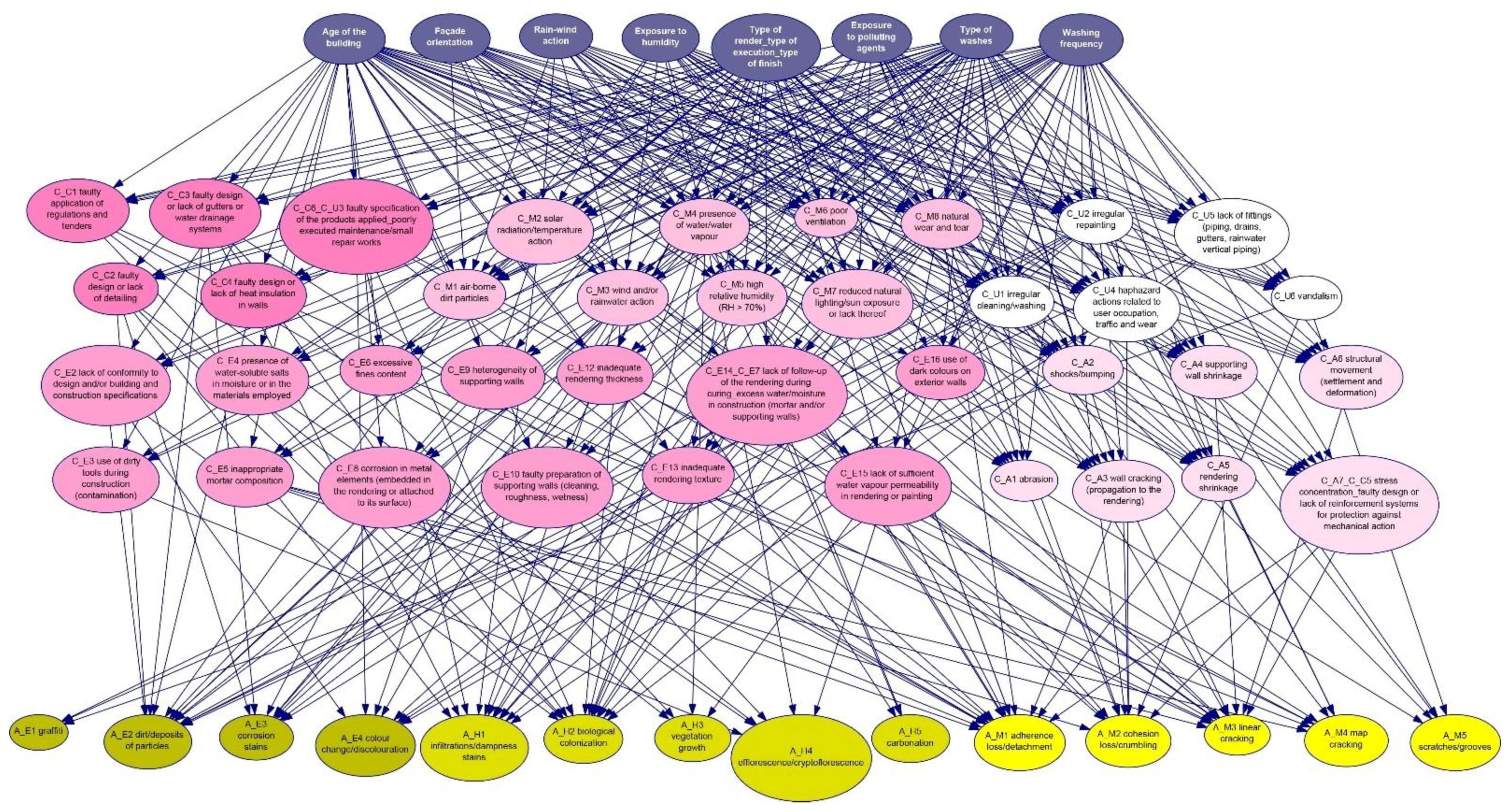
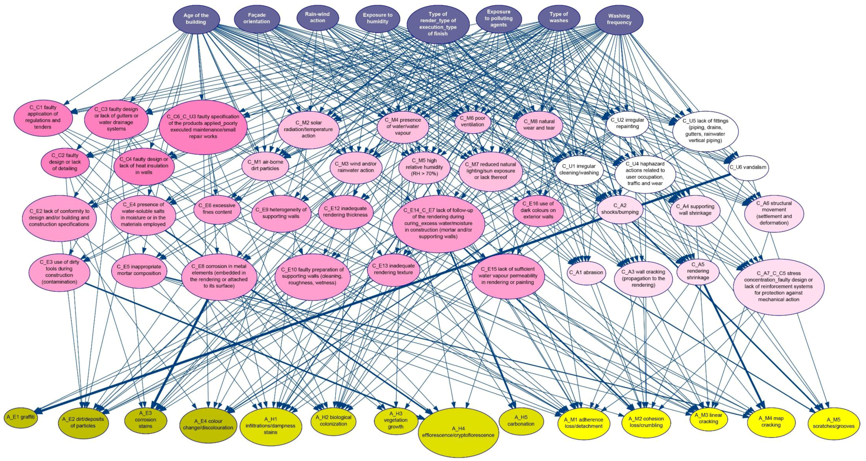
3.1. Development of the Degradation Analysis Model

The variables associated with the degradation of rendered façades in the sample of Sá et al. [19] can be grouped into (i) characteristics of the building and its exposure, (ii) characteristics of the façade and its maintenance, (iii) probable causes of defects, (iv) defects, (v) recommended diagnosis methods and (vi) preconised repair techniques. Within the whole set of variables, to optimise the BN structure and processing time, only some characteristics of the building and of the façade were considered. Moreover, as the network focused on the diagnosis of symptoms and diseases [5], the possibility of carrying out diagnosis methods and the recommendation of repair techniques were excluded from the model. Additionally, selecting variables to frame the problem considered whether they seemed likely to affect the occurrence of defects. The set of variables is presented in

Table 1. Variables in the BN model and respective states (based on [19]).

Variable Designation	Abbreviation	States
Building characteristics and exposure
Age	Age	[2, 10], [11, 19], [20, 27], [28, 35], [36, 43], [44, 51]
Rain–wind action	RaWi	Mild, moderate or harsh
Exposure to humidity	EH	Low or high
Exposure to pollution	EPo	Low, average or high
Façade characteristics and maintenance
Orientation	FaOr	N, NE, E, SE, S, SW, W or NW
Type of render, execution and finish	TyRe/TyEx/Fin	Traditional, manual, textured; traditional, manual, smooth; one coat, mechanical, mineral; or one coat, mechanical, bush hammered
Type of washes	TyWa	Gentle or average
Washing frequency	WaF	Biannual, annual or less frequent
Probable causes of defects
C-C1 Faulty application of regulations and tenders	C-C1	True or false
C-C2 Faulty design or lack of detailing	C-C2	True or false
C-C3 Faulty design or lack of gutters or water drainage systems	C-C3	True or false
C-C4 Faulty design or lack of heat insulation in walls	C-C4	True or false
C-C6 Faulty specification of the products applied/C-U3 Poorly executed maintenance works/minor repairs	C-C6/C-U3	True or false
C-E2 Lack of conformity to design and/or building and construction specifications	C-E2	True or false
C-E3 Use of dirty tools during construction (contamination)	C-E3	True or false
C-E4 Presence of water-soluble salts in moisture or in the materials employed	C-E4	True or false
C-E5 Inappropriate mortar composition	C-E5	True or false
C-E6 Excessive fines content	C-E6	True or false
C-E8 Corrosion in metal elements (embedded in the rendering or affixed to its surface)	C-E8	True or false
C-E9 Heterogeneity of supporting walls	C-E9	True or false
C-E10 Faulty preparation of substrate walls (cleaning, roughness, wetness)	C-E10	True or false
C-E12 Inadequate rendering thickness	C-E12	True or false
C-E13 Inadequate rendering texture	C-E13	True or false
C-E14 Lack of monitoring of the rendering during curing/ C-E7 Excess water/moisture in construction (mortar and/or substrate walls)	C-E14/C-E7	True or false
C-E15 Lack of sufficient water vapour permeability in rendering or painting	C-E15	True or false
C-E16 Use of dark colours in external walls	C-E16	True or false
C-M1 Airborne dirt particles	C-M1	True or false
C-M2 Solar radiation/temperature action	C-M2	True or false
C-M3 Wind and/or rainwater action	C-M3	True or false
C-M4 Presence of water/water vapour	C-M4	True or false
C-M5 High relative humidity (RH > 70%)	C-M5	True or false
C-M6 Poor ventilation	C-M6	True or false
C-M7 Reduced natural lighting/sun exposure or lack thereof	C-M7	True or false
C-M8 Natural wear and tear	C-M8	True or false
C-A1 Abrasion	C-A1	True or false
C-A2 Shocks/bumping	C-A2	True or false
C-A3 Wall cracking (propagation to the rendering)	C-A3	True or false
C-A4 Supporting wall shrinkage	C-A4	True or false
C-A5 Rendering shrinkage	C-A5	True or false
C-A6 Structural motions (settlement and deformation)	C-A6	True or false
C-A7 Stress concentration/C-C5 Faulty design or lack of reinforcement systems for protection against mechanical action	C-A7/C-C5	True or false
C-U1 Irregular cleaning/washing	C-U1	True or false
C-U2 Irregular repainting	C-U2	True or false
C-U4 Accidental actions related to user occupation, traffic and wear	C-U4	True or false
C-U5 Lack of fittings (piping, drains, gutters, rainwater vertical piping)	C-U5	True or false
C-U6 Vandalism	C-U6	True or false
Defects
A-E1 Graffiti	A-E1	True or false
A-E2 Dirt/particle deposits	A-E2	True or false
A-E3 Corrosion stains	A-E3	True or false
A-E4 Colour change/discoloration	A-E4	True or false
A-H1 Infiltration/damp stains	A-H1	True or false
A-H2 Biological colonisation	A-H2	True or false
A-H3 Vegetation growth	A-H3	True or false
A-H4 Efflorescence/cryptoflorescence	A-H4	True or false
A-H5 Carbonation	A-H5	True or false
A-M1 Adhesion loss/detachment	A-M1	True or false
A-M2 Cohesion loss/crumbling	A-M2	True or false
A-M3 Linear cracking	A-M3	True or false
A-M4 Mapped cracking	A-M4	True or false
A-M5 Scratches/grooves	A-M5	True or false

.

Using the Spearman rank-order correlations, non-parametric correlations between the building and façade characteristics were computed. This statistic helped to reduce data, namely joining three different variables (the type of render (e.g., one-coat), type of execution (e.g., mechanical) and type of finish (e.g., bush-hammered)), as they presented high correlation coefficients between them. The type of render and the type of execution had a Spearman rank-order correlation of 1.00, while the type of render and the type of finish had 0.71. The type of execution and the type of finish also had a 0.71 Spearman rank-order correlation. So, in the sample, traditional renders were all executed manually and had two types of finish: textured or smooth. On the other hand, all one-coat renders were executed mechanically and corresponded to two types of finish: mineral or bush hammered.

Pearson product–moment correlations were computed for the probable causes of defects, also aiming at data reduction. High correlations were detected between C-C6 and C-U3 (0.73), C-A7 and C-C5 (0.81) and C-E14 and C-E7 (0.66), which led to pairing those variables. C-C6 refers to the faulty specification of the applied products, while C-U3 refers to poorly executed maintenance works or minor repairs. Although C-U3 refers to the maintenance and operation stage of the building’s life cycle, it is related to C-C6, as poor maintenance and repair works often are due to a poor choice of materials.

As for C-A7, it is a mechanical action cause indicating stress concentration (for instance, next to the corners of windows). That stress can be minimised using reinforcement embedded in the render, and that is what cause C-C5 refers to, thus making sense to join both variables.

Finally, C-E14 is an execution error occurring when there is a lack of monitoring of the rendering during the curing process. On the other hand, C-E7 refers to execution errors while formulating the render, namely with an excessive amount of water or when mortar or substrate walls have excessive moisture. Therefore, knowing that moisture content affects the curing process of the render, C-E14 and C-E7 were paired in a single variable.

High Pearson r correlations were also detected between C-E11 and C-E1, C-E11 and C-E7, C-E11 and C-E14, C-E1 and C-E7, and C-E1 and C-E14. Nevertheless, “C-E11 Rendering applied under adverse weather conditions” and “C-E1 Use of inexperienced/unqualified workmanship” were not observed in the sample of Sá et al. [19], being excluded from the BN structure.

The states of each variable were determined according to the data collected on-site [19]. Buildings were between 2 and 51 years old. Thus, Sturges’ [28] suggestion of sizing intervals was used, as presented in Equation (2):

k = 1 + 3.3 log n

(2)

where n is the number of data values and k is the number of intervals, while logarithms to the base 10 are employed [29]. Six intervals were determined, leading to the presented possible states of the variable “age”.

Rain–wind action, exposure to humidity and exposure to pollution were defined according to the work of Silva et al. [1]. The states of the variable referring to the orientation of the façade were defined according to the cardinal and ordinal directions (eight possible states). The type of render, execution and finish were defined according to the properties of each surface inspected. The type of washes referred to gentle or average aggressiveness in cleaning the façades, while the periodicity of that operation determined three levels of washing frequency.

Table 2. Spearman rank-order correlations between causes and characteristics of buildings and façades.

Causes	Age	FaOr	RaWi	EH	TyRe	TyEx	Fin	EPo	TyWa	WaF
C-C1	−0.12	−0.07	−0.05	0.02	0.07	0.07	0.11	−0.02	0.00	−0.06
C-C2	0.06	0.01	0.05	0.09	0.03	0.03	0.00	0.00	0.01	0.10
C-C3	−0.04	−0.05	−0.05	0.00	−0.05	−0.05	0.03	0.08	−0.09	−0.14
C-C4	−0.01	0.12	0.06	−0.07	−0.01	−0.01	−0.02	−0.04	−0.07	0.16
C-C5	−0.13	0.01	−0.07	0.04	0.01	0.01	0.03	−0.10	−0.05	0.00
C-C6	−0.08	−0.14	−0.09	−0.02	−0.02	−0.02	0.05	−0.08	−0.01	0.08
C-E1	−0.04	−0.11	−0.07	0.07	−0.02	−0.02	0.11	−0.05	−0.03	−0.04
C-E2	−0.06	−0.08	−0.10	0.06	0.02	0.02	0.06	−0.09	0.00	−0.08
C-E3	0.08	−0.05	0.05	0.05	−0.02	−0.02	−0.03	0.10	0.13	−0.03
C-E4	0.02	−0.07	−0.01	−0.05	−0.04	−0.04	0.00	0.05	0.10	0.00
C-E5	−0.04	−0.16	−0.05	0.03	−0.02	−0.02	0.10	−0.12	0.00	0.02
C-E6	0.04	−0.04	0.07	0.05	−0.04	−0.04	0.00	−0.07	0.03	0.00
C-E7	−0.08	−0.13	−0.03	0.09	0.07	0.07	0.15	−0.06	−0.04	−0.05
C-E8	−0.05	−0.02	−0.03	−0.09	−0.09	−0.09	−0.04	−0.10	−0.04	−0.01
C-E9	−0.03	0.05	−0.01	−0.19	0.08	0.08	0.04	−0.08	−0.02	0.14
C-E10	0.08	0.10	0.13	−0.06	−0.06	−0.06	−0.10	0.10	−0.03	−0.07
C-E11	−0.04	−0.11	−0.07	0.07	−0.02	−0.02	0.11	−0.05	−0.03	−0.04
C-E12	0.04	0.14	0.01	−0.11	0.03	0.03	0.00	−0.06	−0.08	0.19
C-E13	−0.04	−0.04	0.01	0.02	0.02	0.02	0.01	0.01	0.02	−0.03
C-E14	−0.11	−0.12	−0.10	0.00	0.14	0.14	0.19	0.00	−0.04	−0.06
C-E15	−0.03	−0.03	0.07	−0.05	−0.04	−0.04	0.00	−0.02	−0.04	−0.06
C-E16	0.04	0.04	−0.07	0.02	0.12	0.12	0.05	0.02	0.03	−0.01
C-M1	−0.04	0.03	0.01	−0.03	−0.03	−0.03	−0.06	−0.02	−0.03	0.03
C-M2	−0.02	0.02	−0.03	−0.09	0.00	0.00	−0.05	−0.08	−0.02	−0.01
C-M3	−0.06	−0.09	−0.06	0.13	0.04	0.04	0.00	−0.04	0.04	−0.04
C-M4	0.02	−0.04	0.06	0.05	−0.11	−0.11	−0.07	0.14	0.08	−0.05
C-M5	0.05	0.15	0.02	0.18	0.07	0.07	0.10	0.07	−0.03	−0.08
C-M6	0.10	−0.14	−0.03	0.03	−0.04	−0.04	0.03	0.05	0.08	0.10
C-M7	0.00	0.06	−0.08	0.06	0.03	0.03	0.03	−0.09	0.00	0.05
C-M8	0.06	−0.02	−0.03	−0.04	−0.03	−0.03	−0.03	−0.03	0.01	−0.06
C-A1	−0.02	−0.10	0.12	0.06	−0.05	−0.05	−0.03	0.00	0.00	−0.08
C-A2	−0.13	−0.19	0.09	0.00	0.09	0.09	0.02	−0.01	0.01	−0.07
C-A3	0.08	0.08	0.10	−0.01	−0.06	−0.06	−0.07	0.21	−0.08	−0.11
C-A4	−0.04	−0.03	−0.07	−0.07	−0.02	−0.02	−0.04	−0.05	−0.03	−0.04
C-A5	0.04	−0.13	−0.05	0.00	−0.06	−0.06	0.05	−0.06	0.03	0.07
C-A6	0.02	0.10	−0.03	−0.09	0.07	0.07	0.04	−0.06	−0.04	−0.05
C-A7	−0.15	−0.02	−0.03	0.02	−0.01	−0.01	0.00	−0.04	−0.04	−0.02
C-U1	−0.06	−0.02	−0.04	0.00	0.08	0.08	0.06	0.07	0.11	−0.02
C-U2	0.00	−0.06	−0.13	−0.06	−0.08	−0.08	−0.03	−0.10	−0.01	0.00
C-U3	0.02	0.03	0.03	−0.01	−0.02	−0.02	0.00	0.02	−0.04	0.10
C-U4	−0.12	−0.08	−0.01	−0.05	0.05	0.05	0.01	−0.07	0.03	0.00
C-U5	−0.05	0.08	−0.06	0.11	0.03	0.03	0.05	−0.10	0.00	−0.08
C-U6	−0.03	−0.01	0.05	−0.07	0.03	0.03	0.10	0.03	−0.06	−0.05

Underlined correlations are significant at p < 0.05. Highlighted correlations: in pink >0.15; in yellow <−0.15. Missing data pairwise deleted.

and

Table 3. Linear correlation between causes and defects.

Causes	A-E1	A-E2	A-E3	A-E4	A-H1	A-H2	A-H3	A-H4	A-H5	A-M1	A-M2	A-M3	A-M4	A-M5
C-C1	−0.07	−0.14	−0.06	−0.09	0.01	−0.06	−0.03	0.09	−0.01	0.02	−0.03	0.45	−0.04	−0.04
C-C2	−0.13	0.17	−0.07	−0.16	0.22	0.22	0.12	−0.05	−0.02	−0.13	−0.05	−0.16	−0.07	−0.08
C-C3	−0.11	0.28	−0.04	−0.14	0.03	0.12	0.04	−0.04	−0.02	−0.07	−0.04	−0.14	−0.06	−0.06
C-C4	−0.05	0.29	−0.04	−0.06	−0.05	−0.06	−0.02	−0.02	−0.01	−0.05	−0.02	−0.06	−0.02	−0.03
C-C5	−0.06	−0.12	−0.05	−0.08	−0.06	−0.08	−0.02	−0.02	−0.01	−0.03	0.05	0.53	−0.03	−0.04
C-C6	−0.09	−0.18	−0.07	0.38	−0.01	−0.10	−0.04	−0.03	−0.02	0.02	−0.03	0.11	0.05	−0.05
C-E1	−0.02	−0.04	−0.02	−0.03	0.24	−0.03	−0.01	−0.01	0.00	−0.02	−0.01	−0.03	−0.01	−0.01
C-E2	−0.04	0.06	−0.03	0.01	0.10	0.00	−0.02	−0.01	−0.01	−0.04	−0.01	−0.05	−0.02	−0.02
C-E3	−0.02	−0.03	−0.01	−0.02	−0.02	−0.02	−0.01	0.50	0.00	−0.01	−0.01	−0.02	−0.01	−0.01
C-E4	−0.03	−0.06	−0.02	−0.04	−0.03	−0.04	−0.01	1.00	−0.01	−0.03	−0.01	−0.04	−0.02	−0.02
C-E5	−0.06	−0.11	−0.04	−0.07	0.00	−0.07	−0.02	−0.02	−0.01	0.11	0.06	−0.02	0.68	−0.03
C-E6	−0.03	−0.06	−0.02	−0.04	−0.03	−0.04	−0.01	−0.01	−0.01	0.28	−0.01	−0.04	0.10	−0.02
C-E7	−0.03	−0.05	−0.02	−0.03	0.22	−0.03	−0.01	−0.01	0.33	−0.02	−0.01	−0.03	−0.01	−0.02
C-E8	−0.07	−0.14	0.93	−0.09	−0.08	−0.10	−0.03	−0.03	−0.01	0.06	−0.03	−0.09	−0.04	−0.04
C-E9	−0.08	0.09	−0.06	−0.10	−0.08	−0.11	−0.03	−0.03	−0.01	−0.08	−0.03	0.42	−0.04	−0.05
C-E10	−0.05	−0.10	−0.04	−0.06	−0.05	−0.07	−0.02	0.08	−0.01	0.56	−0.02	−0.06	−0.03	−0.03
C-E11	−0.02	−0.04	−0.02	−0.03	0.24	−0.03	−0.01	−0.01	0.00	−0.02	−0.01	−0.03	−0.01	−0.01
C-E12	−0.05	0.15	0.04	−0.07	−0.06	−0.07	−0.02	−0.02	−0.01	0.09	−0.02	−0.07	0.10	−0.03
C-E13	−0.07	0.35	−0.06	−0.09	−0.07	−0.01	−0.03	−0.03	−0.01	−0.07	−0.03	−0.09	−0.04	−0.04
C-E14	−0.03	−0.06	−0.02	−0.04	0.16	−0.04	−0.01	−0.01	−0.01	−0.03	0.49	−0.04	−0.02	−0.02
C-E15	−0.03	−0.06	−0.02	−0.04	−0.03	−0.04	−0.01	0.49	−0.01	0.17	−0.01	−0.04	−0.02	−0.02
C-E16	−0.05	−0.09	−0.04	0.42	−0.05	−0.06	−0.02	−0.02	−0.01	−0.05	−0.02	−0.06	−0.02	−0.03
C-M1	−0.17	1.00	−0.13	−0.21	−0.17	−0.22	−0.07	−0.06	−0.03	−0.16	−0.06	−0.21	−0.09	−0.10
C-M2	−0.10	−0.20	−0.08	0.59	−0.04	−0.13	−0.04	−0.04	−0.02	−0.10	−0.04	0.11	0.01	−0.06
C-M3	−0.17	0.44	0.02	−0.08	0.11	−0.06	−0.07	−0.06	0.03	−0.16	0.07	−0.17	−0.08	−0.10
C-M4	−0.15	−0.29	0.21	−0.20	0.13	0.49	0.23	0.20	0.10	0.05	−0.05	−0.17	−0.08	−0.09
C-M5	−0.13	−0.09	0.07	−0.17	0.20	0.34	−0.05	−0.05	−0.02	0.10	−0.01	−0.14	−0.07	−0.08
C-M6	−0.03	−0.06	−0.03	−0.04	0.22	0.00	−0.01	−0.01	−0.01	0.07	−0.01	−0.04	−0.02	−0.02
C-M7	−0.05	−0.11	−0.04	−0.07	0.18	0.25	−0.02	−0.02	−0.01	−0.01	−0.02	−0.07	−0.03	−0.03
C-M8	−0.11	−0.22	−0.01	0.61	−0.07	−0.14	−0.04	−0.04	−0.02	0.08	0.05	−0.06	0.04	−0.07
C-A1	−0.04	−0.08	−0.03	−0.05	−0.04	−0.05	−0.02	−0.01	−0.01	−0.04	0.37	−0.05	−0.02	0.56
C-A2	−0.05	−0.11	−0.04	−0.07	−0.06	−0.07	−0.02	−0.02	−0.01	−0.05	0.28	−0.07	−0.03	0.87
C-A3	−0.06	−0.11	−0.04	−0.07	−0.06	−0.07	−0.02	−0.02	−0.01	0.57	0.05	−0.02	−0.03	−0.03
C-A4	−0.02	−0.04	−0.02	−0.03	−0.02	−0.03	−0.01	−0.01	0.00	−0.02	−0.01	0.20	−0.01	−0.01
C-A5	−0.05	−0.10	−0.04	−0.06	−0.05	−0.07	−0.02	−0.02	−0.01	0.08	−0.02	−0.06	0.89	−0.03
C-A6	−0.03	−0.05	−0.02	−0.03	−0.03	−0.04	−0.01	−0.01	0.00	−0.03	−0.01	0.25	−0.01	−0.02
C−A7	−0.07	−0.14	−0.06	−0.09	−0.07	−0.10	−0.03	−0.03	−0.01	−0.02	−0.03	0.63	−0.04	−0.04
C-U1	0.21	0.01	−0.07	−0.11	−0.09	0.25	0.12	−0.03	−0.02	−0.09	−0.03	−0.11	−0.05	−0.05
C-U2	0.03	0.04	−0.03	0.35	−0.04	−0.15	−0.04	−0.04	−0.02	−0.11	−0.04	−0.14	0.03	0.05
C-U3	−0.06	−0.11	−0.04	0.47	−0.06	−0.07	−0.02	−0.02	−0.01	0.00	−0.02	−0.07	−0.03	−0.03
C-U4	−0.03	−0.06	−0.02	0.04	−0.03	−0.04	−0.01	−0.01	−0.01	−0.03	0.24	−0.04	−0.02	0.29
C-U5	−0.07	−0.01	−0.06	−0.09	0.35	0.11	−0.03	−0.03	−0.01	−0.07	−0.03	−0.09	−0.04	−0.04
C-U6	0.86	−0.19	−0.08	−0.13	−0.10	−0.13	−0.04	−0.04	−0.02	−0.10	0.05	−0.12	−0.05	0.36

Underlined correlations are significant at p < 0.05. Highlighted correlations: >0.70. n = 370 (casewise deletion of missing data).

refer to correlations, respectively, between causes of defects and characteristics of the building and the façade, and between causes of defects and defects.

Although correlation does not imply causality, some affinity is noticed between some parameters in Table 2, as several significant correlations were determined.

In Table 3, the highest correlation coefficients show some empirical relationships, such as the association between graffiti and vandalism; dirt/particles deposits and the existence of airborne dirt particles in the environment; corrosion stains and the corrosion of metal elements, whether embedded or fixed to the surface render; efflorescence/cryptoflorescence and the presence of water-soluble salts; mapped cracking and shrinkage of the render; and scratches/grooves and the occurrence of impacts/bumping with the façade.

The graphical structure of the model reflects the relationships identified in the literature review, namely the characteristics of the building, façade and their exposure influence the rise of diseases (causes of defects), while the causes affect the occurrence of defects. Hence, three levels were designed. The colour of the nodes is also associated with their nature; i.e., first-level nodes are blue, second-level nodes are pink and third-level nodes are yellow. Different shades of pink were used to categorise the nodes of the causes of defects according to the groups of causes [23]: design errors, execution errors, environmental actions, mechanical actions, and wear and maintenance faults. Likewise, different shades of yellow categorised the nodes of defects [23] as aesthetical defects, defects associated with moisture and mechanical action-related defects. The arcs drawn between nodes determined that, to design and execution errors, only the characteristics of the building and façades were relevant, excluding exposure characteristics. The arcs between the causes and the defects were drawn according to the different scenarios of causality determined during the inspection process [19]. Figure 2 represents the graphical structure of the model.

For instance, for node “C-C2 Faulty design or lack of detailing”, the characteristics age, type of render, execution and finish, type of washes and washing frequency were considered to have some influence. Although the maintenance of the façade does not correspond to the design and construction stage of the building’s life cycle, design errors may be highlighted or disguised by the maintenance conditions. As for a node from the group of environmental actions’ causes, “C-M4 Presence of water/water vapour” is considered to be influenced by all first-level nodes. So, it is assumed that the response to aggressive agents is not independent of the building and façade characteristics.

The scenarios of defect occurrence represent the inferences and effect–cause relationships determined by the surveyor during the on-site diagnosis. The example of “A-H1 Infiltrations/dampness stains” can be mentioned. It referred to 20 different combinations of causes, including 12 different types of probable causes (design errors, environmental actions, and wear and maintenance faults). Still, the Noisy-Max assumption [20] determines that each cause must be considered as being able to produce the effect (defect) separately. Thus, it is assumed that the surveyor determines more than one cause for an occurrence as a reflection of the uncertainty of the diagnosis.

The CPTs of the nodes mirror the specificity of the sample of Sá et al. [19], i.e., construction features are associated with the Portuguese construction sector methodologies and practices, while environmental specifications are typical of a metropolitan area with a Mediterranean climate. Relative frequencies were used as the probability measure. Figure 3 shows an excerpt of the BN model, where nodes are represented by boxes showing bar charts of the probability of each node. It is noted that “C-M1 Airborne dirt particles” (88%) is the most probable cause in the group of environmental actions. Additionally, in the first-level nodes, the prevalence of gentle washes (85%) on the sample of façades is evident.

3.2. Model Evaluation

3.2.1. Verification of the Model Results

To verify the estimation of uncertainty in the diagnosis process, inspection results from a different sample [27] were used. In the BN model, the characteristics of the building were input, as well as the detected defects, one at a time. The unequivocal presence or absence of causes was also entered, namely the absence of vandalism. One building was chosen, and a surface per inspected façade was analysed. The results and the quantification of uncertainty provided by the BN are presented in

Table 4. Quantification of uncertainty based on the BN model using cases of a sample from the literature [27].

Input Data	Input Defect (Detected by the Surveyor)	Causes (Pointed Out by the Surveyor)	p (True)— Uncertainty Measure
- Age: [2,10] - FaOr: SW - RaWi: Moderate - EH: Low - TyRe/TyEx/Fin: Traditional, manual, smooth - EPo: High - C-U6: False	A-H1 Infiltration/damp stains	C-M4 Presence of water/water vapour	85%
		C-C6 Faulty specification of the products applied/C-U3 Poorly executed maintenance works/minor repairs	43%
	A-H4 Efflorescence/cryptoflorescence	C-C2 Faulty design or lack of detailing	39%
		C-E4 Presence of water-soluble salts in moisture or in the materials employed	28%
		C-E14 Lack of monitoring of the rendering during curing/ C-E7 Excess water/moisture in construction (mortar and/or substrate walls)	14%
		C-M4 Presence of water/water vapour	87%
		C-C6 Faulty specification of the products applied/C-U3 Poorly executed maintenance works/minor repairs	43%
	A-M3 Linear cracking	C-M2 Solar radiation/temperature action	58%
		C-M8 Natural wear and tear	62%
		C-A7 Stress concentration/C-C5 Faulty design or lack of reinforcement systems for protection against mechanical action	67%
	A-M4 Mapped cracking	C-M8 Natural wear and tear	65%
		C-A7 Stress concentration/C-C5 Faulty design or lack of reinforcement systems for protection against mechanical action	62%
- Age: [2,10] - FaOr: SE - RaWi: Moderate - EH: Low - TyRe/TyEx/Fin: Traditional, manual, smooth - EPo: High - C-U6: False	A-H1 Infiltration/damp stains	C-C2 Faulty design or lack of detailing	61%
		C-C3 Faulty design or lack of gutters or water drainage systems	49%
		C-M8 Natural wear and tear	63%
	A-M3 Linear cracking	C-M2 Solar radiation/temperature action	58%
		C-A7 Stress concentration/C-C5 Faulty design or lack of reinforcement systems for protection against mechanical action	65%
	A-M1 Adhesion loss/detachment	C-E8 Corrosion in metal elements (embedded in the rendering or affixed to its surface)	31%
		C-A7 Stress concentration/C-C5 Faulty design or lack of reinforcement systems for protection against mechanical action	59%
- Age: [2,10] - FaOr: NE - RaWi: Moderate - EH: Low - TyRe/TyEx/Fin: Traditional, manual, smooth - EPo: High - C-U6: False	A-H1 Infiltration/damp stains	C-C2 Faulty design or lack of detailing	39%
		C-M8 Natural wear and tear	63%
		C-C6 Faulty specification of the products applied/C-U3 Poorly executed maintenance works/minor repairs	43%
		C-U5 Lack of fittings (piping, drains, gutters, rainwater vertical piping)	33%
	A-M5 Scratches/grooves	C-A2 Shocks/bumping	61%
		C-C6 Faulty specification of the products applied/C-U3 Poorly executed maintenance works/minor repairs	43%
- Age: [2,10] - FaOr: NW - RaWi: Moderate - EH: Low - TyRe/TyEx/Fin: Traditional, manual, smooth - EPo: High - C-U6: False	A-H1 Infiltration/damp stains	C-C2 Faulty design or lack of detailing	39%
		C-C3 Faulty design or lack of gutters or water drainage systems	51%
		C-C4 Faulty design or lack of heat insulation in walls	11%
		C-E2 Lack of conformity to design and/or building and construction specifications	11%
		C-M4 Presence of water/water vapour	87%
		C-M5 High relative humidity (RH > 70%)	75%
		C-M7 Reduced natural lighting/sun exposure or lack thereof	29%
		C-C6 Faulty specification of the products applied/C-U3 Poorly executed maintenance works/minor repairs	43%

.

The building selected was eight years old at the moment of inspection and was subjected to moderate wind–rain action. It had low exposure to humidity and high exposure to polluting agents. The façades were rendered with a traditional mortar scheme, applied manually with a smooth finish. No information was available referring to the type of washes nor its frequency. As the building was in a fenced plot, “C-U6 Vandalism” was considered to be false.

The uncertainty of the causes of defects shown in Table 4 express that:

• Design and execution errors’ causes have consistently lower probabilities of being true.
• Every set of causes selected for a defect has at least one cause with a probability of being true higher than 50%.
• The highest probability obtained from the verification cases was 87%, corresponding to cause “presence of water/water vapour” (C-M4) of defects “efflorescence/cryptoflorescence” (A-H4) and “infiltration/damp stains” (A-H1); this cause is a well-known part of the degradation mechanism of efflorescence and façade staining [30].
• The lowest probability obtained from the verification cases was 11%, corresponding to causes “faulty design or lack of heat insulation in walls” (C-C4) and “lack of conformity to design and/or building and construction specifications” (C-E2), attributed to the occurrence of “infiltration/damp stains” (A-H1). When thermophoresis occurs (i.e., the condensation of water vapour in the cooler areas/materials of a façade [31]), the design of a poorly insulated wall or not executing the designed wall (well insulated) may result in moisture stains highlighted by the accumulation of dirt; however, through a merely visual inspection, those causes cannot be confirmed, hence the high level of uncertainty.

From this brief verification, it can be concluded that the uncertainty results are consistent with the surveyor’s reservations during the diagnosis process.

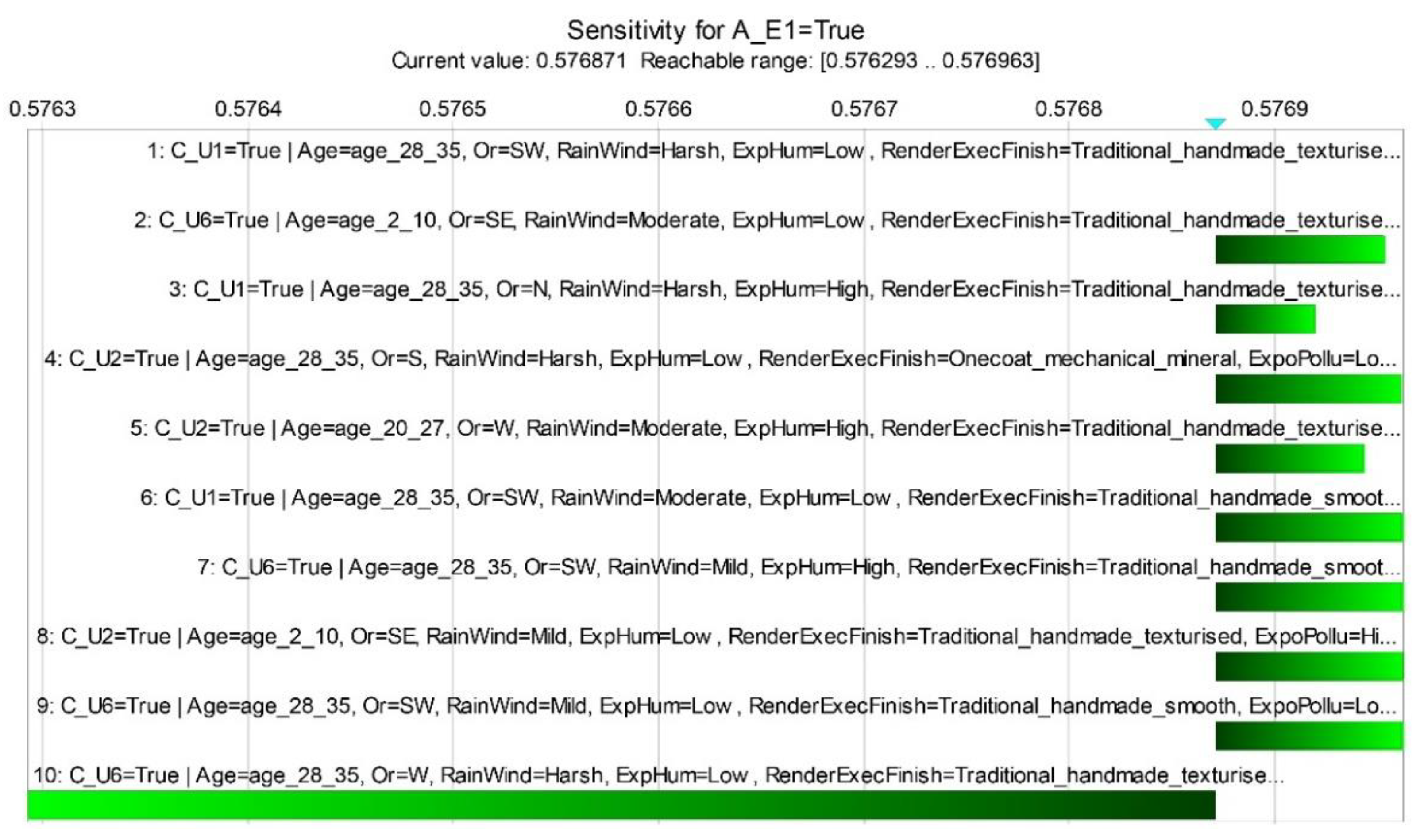
3.2.2. Sensitivity Analysis

Before proceeding to perform a sensitivity analysis, a strength-of-influence diagram was drawn (Figure 4), where arcs have different thicknesses, depending on the amount of impact that nodes exert on other nodes. It expresses the distance between various conditional probability distributions over the child node conditional on the states of the parent node [32]. To obtain this diagram, the Euclidean measure of distance between distributions was used [8], and the average distances were displayed.

From the strength-of-influence diagram, these are the most influential relationships:

• The influence of C-E8 on A-E3 is the strongest, associating the corrosion of metal elements with the appearance of corrosion stains [33,34].
• Then, vandalism (cause) is highly related to the observation of graffiti (effect) [35,36].
• The occurrence of mapped cracking (defect A-M4) is significantly influenced by the shrinkage of the render (cause C-A5) [37,38].
• The lack of follow-up activities when the render is curing or the existence of excessive construction moisture (C-E14/C-E7) reflects on the occurrence of cohesion loss/crumbling (A-M2) [39,40].

It is coherent that the most relevant influences are supported by the literature [33,34,35,36,37,38,39,40,41] since the inspection system of Sá et al. [23] is based on a review of the knowledge on the degradation of rendered walls and on the experience of experts.

The sensitivity analysis also contributed to the verification of the BN model. This type of analysis provides a visual perspective and helps to locate the most sensitive parameters, depending on the context (target nodes set). Six nodes were identified as targets, referring to the six most frequent defects in the samples of Sá et al. [19]: “A-E1 Graffiti”, “A-E2 Dirt/particle deposits”, “A-E4 Colour change/discolouration”, “A-H1 Infiltration/damp stains”, “A-H2 Biological colonisation” and “A-M3 Linear cracking”. The colour scale of the diagram identified A-E1 (average sensitivity = 0.063, maximum = 0.205) and A-E4 (average sensitivity = 0.002, maximum = 0.125) as the most sensitive nodes. Still, in the set of first-level nodes, the age of the building was also identified as a significant sensitive node; i.e., it is important for the calculation of probability distributions in the nodes marked as targets.

Tornado diagrams were drawn for both “A-E1 Graffiti” and “A-E4 Colour change/discolouration” (Figure 5 and Figure 6, respectively). Such diagrams present the most sensitive parameters for a predetermined state of the target node. The length of each bar refers to the range of changes that a parameter can produce in the state of the target node. The red colour represents negative change, while green represents positive change.

In Figure 5, the tornado diagram representing the sensitivity of node A-E1 shows the impact of the combination of vandalism (C-U6) being true, a building being 28–35 years old, orientation towards the west, harsh rain–wind action exposure and low exposure to humidity. In fact, the only important condition in this set of characteristics is the occurrence of vandalism. However, as the combination of characteristics is always identified, they are all highlighted in this analysis. Vandalism (C-U6) being true is also present in two more parameters of Figure 5. The tornado diagram ranges from 0.576293 to 0.576963, thus still referring to low levels of sensitivity.

The tornado diagram for colour changes/discolouration (A-E4), in Figure 6, shows in turn the relevant impact of the occurrence of natural wear and tear (C-M8), the building being 28–35 years old, orientation towards SW, harsh exposure to rain–wind action and low exposure to humidity. Still, the range of the diagram is only 0.00001.

3.2.3. Case Study

A residential building in Portugal was randomly selected to validate the proposed model. It was built in 1984 and has two floors and a floor area of 176 m². The building’s rendered façades were already subjected to maintenance actions (repainting), not including minor repairs in the render layer. The building has a reinforced concrete structure with ceramic brick masonry walls and a two-slope pitched roof with eaves. The windowsills are protruding elements on the façades, and they include a drip detail on their lower surface. The main façade (northeast) is only one floor high, as the lower floor is essentially a basement, with exterior walls northwest, southwest and southeast.

Table 5. Evidence for nodes related to the characteristics of the building, the façade and their exposure conditions, as well as cause C-U6.

Node	State
Age of the building	36–43 years
Façade orientation	NW, NE, SE and SW
Rain–wind action	Harsh
Exposure to humidity	Low
Type of render/type of execution/type of finish	Traditional/manual/smooth
Exposure to polluting agents	High
C-U6 Vandalism	False

Note: Selected nodes refer to known facts about the case study.

identifies the state of the evidence nodes for the case study building.

A technical inspection based only on visual observation was performed on the building with the mere purpose of identifying the occurrence of defects. The observed defects were:

• A-E2 Dirt/particle deposits
• A-H1 Infiltration/damp stains
• A-H2 Biological colonisation
• A-M1 Adhesion loss/detachment
• A-M3 Linear cracking
• A-M4 Mapped cracking
• A-M5 Scratches/grooves.

This set of defects should be compared with the prediction of the model, presented in

Table 6. Defect occurrence results.

Defect	Occurrence
	True	False
A-E1 Graffiti	28–30%	70–72%
A-E2 Dirt/particle deposits	99%	1%
A-E3 Corrosion stains	52–53%	47–48%
A-E4 Colour change/discolouration	80–81%	19–20%
A-H1 Infiltration/damp stains	58–61%	39–42%
A-H2 Biological colonisation	84–86%	14–16%
A-H3 Vegetation growth	12–13%	87–88%
A-H4 Efflorescence/cryptoflorescence	15%	85%
A-H5 Carbonation	3%	97%
A-M1 Adhesion loss/detachment	68–69%	31–32%
A-M2 Cohesion loss/crumbling	19–21%	79–81%
A-M3 Linear cracking	79–81%	19–21%
A-M4 Mapped cracking	34–37%	63–66%
A-M5 Scratches/grooves	28–33%	67–72%

.

Considering the defects with a probability of occurrence higher than 50% (Table 6), only corrosion stains were not identified in the case study building. On the other hand, both mapped cracking and scratches/grooves were present in one or more surfaces of the case study, although the model only predicted a 34–37% and 28–33% chance of occurrence, respectively. Mapped cracking occurs on the northwest façade and was not repaired before repainting. The detected scratches/grooves are due to vehicle bumping next to the garage entrance.

Additionally, the causes of defects with a probability of occurrence higher than 50% in the BN model are (Figure 7):

• C-M1 Airborne dirt particles
• C-M2 Solar radiation/temperature action
• C-M3 Wind and/or rainwater action
• C-M4 Presence of water/water vapour
• C-M5 High relative humidity (RH > 70%)
• C-M8 Natural wear and tear
• C-U1 Irregular cleaning/washing
• C-U2 Irregular repainting

All these causes correspond to reasonably inferred causes of the detected defects. Nevertheless, some causes may be missing from the presented list, such as “C-A2 Shocks/bumping” (16% probability), “C-A5 Rendering shrinkage (17%), “C-A6 Structural motions (settlement and deformation)” (6%), “C-A7 Stress concentration/C-C5 Faulty design or lack of reinforcement systems for protection against mechanical action” (43%) and “C-U4 Accidental actions related to user occupation, traffic and wear” (10%). These causes mainly refer to mechanical action, requiring further tests for confirmation (e.g., tell-tale crack gauge); thus the high level of uncertainty may not be completely out of step with reality. Even so, the experience of surveyors could compensate for such high levels of uncertainty. Furthermore, some information observed on-site that is not included in the variables may also explain the high levels of uncertainty. C-U4 corresponds to an accidental cause that can only be confirmed by witnesses or a complete set of maintenance records. Hence, the sample of Sá et al. [19] and their inspection conditions may be limiting the BN model.

4. Discussion

Although uncertainty is inherent to the diagnosis of building degradation, depending on the amount and quality of available data, on the inspection methodology and on the experience and knowledge of the surveyor, the quantification of such uncertainty is not immediate. The methods used in this research allowed the authors to propose a model to measure uncertainty while assessing the degradation of rendered façades. The model was developed on the grounds of an existing building inspection system [19,23] based on expert knowledge and experience. The provided systematisation of deterioration mechanisms and inspection data, following the best practices in the field [42], was a solid basis for the current study. Additionally, Sá et al. [19] provided thorough information on the characteristics of the inspected buildings and supplied a representative sample size. The variables selected as important attributes of the analysed built objects have also been considered by other authors that studied building pathology [43,44,45,46,47,48,49,50,51,52].

Nevertheless, as the sample [19] used to determine the CPTs was the same that had been used to validate the building inspection system [23], any minor incorrection not detected by those authors may have been transposed to the BN model. Additionally, that same sample does not have universal representativeness. Although it is representative of the Portuguese population of rendered façades, its applicability to other construction and environmental contexts may require further analysis, namely in terms of substrate materials (in the sample, masonry and concrete), the materials’ content of mortars (cement, lime, water and admixtures), exposure to weather agents according to climatic features and current maintenance activities (in the sample, only the type of washes and its frequency were considered).

The proposed model supplies a graphical representation of quantitative and qualitative data that is easy to interpret, focusing on the cause–defect relationship. BN models have also been used by other authors with similar purposes, for instance, evaluation of maintenance scenarios [16], making predictive maintenance decisions [9,10], inspection planning in ships [53], damage assessment [54] and design-for-maintainability assessment of building systems [17]. Yet, to the best of the authors’ knowledge, no other research has centred on the use of BN models to analyse the diagnosis process of building defects on rendered façades.

Nevertheless, the developed BN should not be viewed as a diagnosis guide, considering the probabilities as the basis for assuming the presence of defects or their causes. Instead, the proposed model should complement the in situ diagnosis process as an additional source of information or quantification tool. It should not be downplayed that an event with a 1% chance of occurrence may still be observed three times when the sample has 300 cases. So, if there is only a 1% chance of a rendered façade not presenting “A-E2 Dirt/particle deposits”, surveyors should not assume that such defect is observed in all the façades they inspect.

The verification of the uncertainty estimates using data from a different inspection sample shows that the proposed model is valid, providing uncertainty levels consistent with the surveyor’s diagnosis process. Additionally, a strength-of-influence diagram was drawn to identify the most influential relationships between nodes. Those relationships correspond to associations recognised in the literature as part of degradation mechanisms. Furthermore, to check which variables had the highest impact on selected target nodes [20], a sensitivity analysis was performed. It confirmed that the probability of occurrence of graffiti (A-E1) is more sensitive to changes in the state of variable vandalism (C-U6), while the probability of occurrence of colour changes/discolouration (A-E4) is more sensitive to changes in the states of natural wear and tear (C-M8), age of the building, the orientation of the façade, exposure to rain–wind action and exposure to humidity. These results are in line with studies on façade pathology [1,33,34,35,36,37,40,41,43,44,45,46,47,52].

The analysis of the case study highlighted that the detected defects had been predicted by the proposed BN model with reasonable levels of uncertainty, as only two of the detected defects had a probability of occurrence lower than 50%. On the other hand, the most probable causes predicted by the model were likely to cause the detected defects, but some causes that could be identified during the diagnosis process had lower probabilities (between 6% and 43%). Nevertheless, those high levels of uncertainty are justified by the need of further testing or additional information to confirm the occurrence of the selected causes.

Given the development of other inspection systems [42], and their validation in representative samples, the proposed model can be replicated for other building materials or elements, provided that the necessary adaptations are taken into account. Still, the time/effort required to compute the BN model may limit the expected technological advance. The complexity of buildings in terms of variety of materials, elements and systems may also limit a wider scope of BN models in terms of degradation mechanisms, since it may be difficult to collect and use significant samples of information on all types of materials, elements or systems. Even so, Bayes’ belief networks could still be built, considering the assessment of experts, estimating the probability of events [10,20].

Additionally, the proposed model could be extended with the inclusion of more variables and levels of analysis. For instance, the height of the building could be included as one of the properties of the rendered surface, and recommended in situ diagnosis methods and repair techniques could be included in a new (fourth) level of variables. That was not the case in the current research, because the proposed approach required an initial validation step, which is presented in this paper. The future inclusion of new variables in the network may expand its scope of interest.

With the possibilities provided by computer applications for building inspection [42,55,56,57], in the future, this network may be used to integrate data and provide more tools for surveyors during the inspection procedures. Furthermore, the integration of several BN models referring to the degradation of different materials may become a powerful instrument to relate degradation in adjacent elements or systems.

5. Conclusions

Building inspection and diagnosis involves uncertainty while simultaneously analysing numerous variables. Although surveyors are normally conscious of that uncertainty, it is difficult to quantify it. Therefore, this paper proposes the development of a new BN model to quantify uncertainty in the diagnosis of defects and their causes during technical inspections. Rendered façades were used to develop the prototype model. Bayesian networks are a well-supported framework for uncertainty reasoning that allow constructing coherent probabilistic representations. Those conditional probabilities can be based on available databases with a large number of cases or on assessments of probability obtained from experts [20,22]. In this paper, a database was used.

The proposed model includes a well-structured and comprehensive representation of cause–effect relationships affecting building pathology in façade renders, offering a new approach/analysis to previously published data [19]. The model is limited to the main characteristics of the building, façade and their exposure; the causes of defects; and the defects that may be observed in rendered façades. Additionally, it represents a balance between complexity and computation time.

The probability distributions of variables were defined according to a dataset from the literature [19], thus representing a specific population (building characteristics and exposure conditions). Nevertheless, degradation patterns should be similar to those in other contexts.

The validation of results confirmed the model, as the estimates of uncertainty are a good depiction of the surveyor’s reservations during the diagnosis process, as demonstrated by using cases from another sample and a new case study. In this way, the causes in the groups of design and execution errors were associated with higher levels of uncertainty, since information about the design and execution processes (often missing) may be required to establish causal relationships of defects to events at those initial stages. Additionally, some causes in the group of mechanical actions were also associated with high levels of uncertainty, since their identification may lack confirmation through the use of in situ tests.

Furthermore, the relative importance of different indicants, as revealed by a strength-of-influence diagram and sensitivity analysis, was supported by the literature about degradation mechanisms on rendered façades. In the model, expected relationships were clearly identified through the mentioned analyses, such as the influence of corrosion of metal elements on the appearance of corrosion stains, the influence of vandalism on the occurrence of graffiti and the influence of render shrinkage on the occurrence of mapped cracking.

The proposed model may help surveyors to provide better information to decision makers, thus promoting better repair and maintenance choices.

Future studies could include the replication of the proposed methodology for other building materials or elements, the extension of the model with more variables and levels of analysis and the integration of the model in building inspection computer applications.

References

1. Silva, A.; de Brito, J.; Gaspar, P.L. Methodologies for Service Life Prediction of Buildings. With a Focus on Façade Claddings; Green Energy and Technology; Springer: Cham, Switzerland, 2016; ISBN 978-3-319-33288-8. [Google Scholar]
2. Flores-Colen, I.; de Brito, J. A systematic approach for maintenance budgeting of buildings façades based on predictive and preventive strategies. Constr. Build. Mater. 2010, 24, 1718–1729. [Google Scholar] [CrossRef]
3. Pereira, C.; Silva, A.; de Brito, J.; Ferreira, C.; Flores-Colen, I.; Silvestre, J.D. Uncertainty and risk analysis in inspection and diagnosis. In New Trends on Building Pathology, CIB W86 Report; CIB International Council for Research and Innovation in Building and Construction: Lisboa, Portugal, 2021. [Google Scholar]
4. Flores-Colen, I.; de Brito, J.; de Freitas, V.P.; Hawreen, A. Reliability of in-situ diagnosis in external wall renders. Constr. Build. Mater. 2020, 252, 119079. [Google Scholar] [CrossRef]
5. Wolf, F.M.; Gruppen, L.D.; Billi, J.E. Differential diagnosis and the competing-hypotheses heuristic. A practical approach to judgement under uncertainty and Bayesian probability. J. Am. Med. Assoc. 1985, 253, 2858–2862. [Google Scholar] [CrossRef]
6. Weber, P.; Simon, C. Benefits of Bayesian Network Models; Systems and industrial engineering series—Systems dependability assessment set; ISTE Wiley: London, UK, 2016; ISBN 9781848219922. [Google Scholar]
7. Verron, S.; Tiplica, T.; Kobi, A. Monitoring of complex processes with Bayesian networks. In Bayesian Network; Rebai, A., Ed.; Sciyo: Rijeka, Croatia, 2010; pp. 213–227. ISBN 978-953-307-124-4. [Google Scholar]
8. Koiter, J.R. Visualizing Inference in Bayesian Networks. Master’s Thesis, Faculty of Electrical Engineering, Mathematics, and Computer Science, Delft University of Technology, Delft, The Netherlands, 16 June 2006. [Google Scholar]
9. Bortolini, R.; Forcada, N. Discussion about the use of Bayesian networks models for making predictive maintenance decisions. In Proceedings of the Joint Conference on Computing in Construction (JC3), Heraklion, Greece, 4–12 July 2017; pp. 973–980. [Google Scholar]
10. Bortolini, R.; Forcada, N. A probabilistic performance evaluation for buildings and constructed assets. Build. Res. Inf. 2020, 48, 838–855. [Google Scholar] [CrossRef]
11. Bortolini, R.; Forcada, N. Operational performance indicators and causality analysis for non-residential buildings. Inf. la Construcción 2020, 72, 1–11. [Google Scholar]
12. Luque, J.; Straub, D. Reliability analysis and updating of deteriorating systems with dynamic Bayesian networks. Struct. Saf. 2016, 62, 34–46. [Google Scholar] [CrossRef]
13. Schneider, R.; Fischer, J.; Bügler, M.; Nowak, M.; Thöns, S.; Borrmann, A.; Straub, D. Assessing and updating the reliability of concrete bridges subjected to spatial deterioration - Principles and software implementation. Struct. Concr. 2015, 16, 356–365. [Google Scholar] [CrossRef]
14. Gallina, G.; Graziosi, M.; Imbrenda, A. Structural repair approach for reinforcement corrosion in concrete building structure: An application case. In Proceedings of the 4th International Conference on Concrete Repair, Rehabilitation and Retrofitting (ICCRRR 2015), Leipzig, Germany, 5–7 October 2015; Dehn, F., Beushausen, H.-D., Alexander, M.G., Moyo, P., Eds.; CRC Press: Leipzig, Germany, 2015; pp. 695–702. [Google Scholar]
15. Vagnoli, M.; Remenyte-Prescott, R.; Andrews, J. Structural health monitoring of bridges: A Bayesian network approach. In Proceedings of the Life-Cycle Analysis and Assessment in Civil Engineering: Towards an Integrated Vision, Ghent, Belgium, 28–31 October 2018; Caspeele, R., Taerwe, L., Frangopol, D., Eds.; Taylor & Francis: Ghent, Belgium, 2018; pp. 1983–1989. [Google Scholar]
16. Sivo, M.; Ladiana, D.; Novi, F.; Salvatori, C. Maintenance-oriented design in architecture. A decision support system for the evaluation of maintenance scenarios through Bayesian networks use. A case study: The headquarters of ING groupe in Amsterdam. In Proceedings of the XV International Conference on Durability of Building Materials and Components, Barcelona, Spain, 20–23 October 2020; Serrat, C., Casas, J.R., Gibert, V., Eds.; International Center for Numerical Methods in Engineering (CIMNE): Barcelona, Spain, 2020; pp. 1695–1702. [Google Scholar]
17. Asmone, A.S.; Chew, M.Y.L. Development of a design-for-maintainability assessment of building systems in the tropics. Build. Environ. 2020, 184, 107245. [Google Scholar] [CrossRef]
18. BayesFusion LLC. GeNIe Academic, Version 3.0.6518.0 (32-bit); BayesFusion LLC: Pittsburgh, PA, USA, 2021. [Google Scholar]
19. Sá, G.; Sá, J.; de Brito, J.; Amaro, B. Statistical survey on inspection, diagnosis and repair of wall renderings. J. Civ. Eng. Manag. 2015, 21, 623–636. [Google Scholar] [CrossRef] [Green Version]
20. Henrion, M. Practical issues in constructing a Bayes’ belief network. Int. J. Approx. Reason. 1988, 2, 132–139. [Google Scholar]
21. Garcia, J.; de Brito, J. Inspection and diagnosis of epoxy resin industrial floor coatings. J. Mater. Civ. Eng. 2008, 20, 128–136. [Google Scholar] [CrossRef]
22. Díez, F.J. Parameter adjustment in Bayes networks. The generalized noisy OR–gate. In Proceedings of the Ninth international conference on Uncertainty in artificial intelligence (UAI’93), Washington, DC, USA, 9–11 July 1993; Heckerman, D., Mamdani, A., Eds.; Morgan Kaufmann Publishers Inc.: Washington, DC, USA, 1993; pp. 99–105. [Google Scholar]
23. Sá, G.; Sá, J.; de Brito, J.; Amaro, B. Inspection and diagnosis system for rendered walls. Int. J. Civ. Eng. 2014, 12, 279–290. [Google Scholar]
24. StatSoft Inc. STATISTICA (Data Analysis Software System), Version 8.0; StatSoft Inc.: Tulsa, OK, USA, 2007. [Google Scholar]
25. Bashari, H.; Smith, C.S. Accommodating uncertainty in grazing land condition assessment using Bayesian Belief Networks. In Bayesian Network; Rebai, A., Ed.; Sciyo: Rijeka, Croatia, 2010; pp. 341–354. ISBN 978-953-307-124-4. [Google Scholar]
26. Engel, A. Verification, Validation, and Testing of Engineered Systems; Wiley series in systems engineering and management; Wiley: Hoboken, NJ, USA, 2010; ISBN 978-0-470-52751-1. [Google Scholar]
27. Pereira, C.; Silva, A.; de Brito, J.; Silvestre, J.D. Urgency of repair of building elements: Prediction and influencing factors in façade renders. Constr. Build. Mater. 2020, 249, 118743. [Google Scholar] [CrossRef]
28. Sturges, H.A. The choice of a class interval. J. Am. Stat. Assoc. 1926, 21, 65–66. [Google Scholar] [CrossRef]
29. Benjamin, J.R.; Cornell, C.A. Probability, Statistics, and Decision for Civil Engineers; Dover Publications, Inc.: Mineola, NY, USA, 2016; ISBN 978-0-486-78072-6. [Google Scholar]
30. Pereira, C.; de Brito, J.; Silvestre, J.D. Global inspection, diagnosis and repair system for buildings: Managing the level of detail of the defects classification. In Proceedings of the Rehabend—Construction Pathology, Rehabilitation Technology and Heritage Management, Caceres, Spain, 15–18 May 2018; Villegas, L., Lombillo, I., Blanco, H., Boffil, Y., Eds.; University of Cantabria; University of Extremadura: Cáceres, Spain, 2018; pp. 572–579. [Google Scholar]
31. Camuffo, D. Microclimate for Cultural Heritage: Conservation, Restoration, and Maintenance of Indoor and Outdoor Monuments, 2nd ed.; Elsevier: Boston, MA, USA, 2014; ISBN 9780444632968. [Google Scholar]
32. BayesFusion LLC Strength of Influences. Available online: https://support.bayesfusion.com/docs/GeNIe/ (accessed on 9 June 2021).
33. Flores-Colen, I.; de Brito, J.; Freitas, V.P. de Stains in facades’ rendering— Diagnosis and maintenance techniques’ classification. Constr. Build. Mater. 2008, 22, 211–221. [Google Scholar] [CrossRef]
34. Norvaišienė, R.; Miniotaitė, R.; Stankevičius, V. Climatic and air pollution effects on building facades. Mater. Sci. 2003, 9, 102–105. [Google Scholar]
35. Carvalhão, M.; Dionísio, A. Evaluation of mechanical soft-abrasive blasting and chemical cleaning methods on alkyd-paint graffiti made on calcareous stones. J. Cult. Herit. 2015, 16, 579–590. [Google Scholar] [CrossRef]
36. Weaver, M.E. Removing Graffiti from Historic Masonry; Preservation Briefs 38; U.S. Department of the Interior, National Park Service Cultural Resources, Preservation Assistance: Washington, DC, USA, 1995.
37. Douglas, J.; Ransom, B. Understanding Building Failures, 3rd ed.; Taylor & Francis: London, UK, 2007; ISBN 0415370825. [Google Scholar]
38. Bussel, M. Effects of induced movement. In Structures & Construction in Historic Building Conservation; Forsyth, M., Ed.; Blackwell Publishing: Oxford, UK, 2007; pp. 111–139. ISBN 9781405111713. [Google Scholar]
39. Sazedj, S.; Morais, A.; Pinheiro-Alves, M.T.; Silva, R. Pathologies—Incompatibility of materials and human intervention in a historic building of Elvas. In New Approaches to Building Pathology and Durability; Delgado, J.M.P.Q., Ed.; Springer: Singapore, 2016; Volume 6, ISBN 978-981-10-0647-0. [Google Scholar]
40. Flores-Colen, I.; de Brito, J. Renders. In Materials for Construction and Civil Engineering: Science, Processing, and Design; Gonçalves, M.C., Margarido, F., Eds.; Springer: Cham, Switzerland, 2015; pp. 53–122. ISBN 978-3-319-08235-6. [Google Scholar]
41. Honeyborne, D.B. Weathering and decay of masonry. In Conservation of Building and Decorative Stone; Ashurst, J., Dimes, F.G., Eds.; Butterworth-Heinemann: Oxford, UK, 1998; pp. 153–184. ISBN 9780750638982. [Google Scholar]
42. Ferraz, G.T.; de Brito, J.; de Freitas, V.P.; Silvestre, J.D. State-of-the-art review of building inspection systems. J. Perform. Constr. Facil. 2016, 30, 04016018. [Google Scholar] [CrossRef]
43. Silva, A.; de Brito, J.; Gaspar, P.L. A comparative multi-criteria decision analysis of service life prediction methodologies for rendered façades. J. Build. Eng. 2018, 20, 476–487. [Google Scholar] [CrossRef]
44. Vieira, S.M.; Silva, A.; Sousa, J.M.C.; De Brito, J.; Gaspar, P.L. Modelling the service life of rendered facades using fuzzy systems. Autom. Constr. 2015, 51, 1–7. [Google Scholar] [CrossRef]
45. Ferreira, C.; Barrelas, J.; Silva, A.; de Brito, J.; Dias, I.S.; Flores-Colen, I. Impact of environmental exposure conditions on the maintenance of facades’ claddings. Buildings 2021, 11, 138. [Google Scholar] [CrossRef]
46. Gaspar, P.L.; de Brito, J. Service life estimation of cement-rendered facades. Build. Res. Inf. 2008, 36, 44–55. [Google Scholar] [CrossRef]
47. Silva, A.; de Brito, J.; Gaspar, P.L. Stochastic approach to the factor method: Durability of rendered façades. J. Mater. Civ. Eng. 2015, 28, 04015130. [Google Scholar] [CrossRef]
48. Júnior, C.M.M.; Carasek, H. Relationship between the deterioration of multi story buildings facades and the driving rain. Rev. la Construcción 2014, 13, 64–73. [Google Scholar] [CrossRef] [Green Version]
49. Al-Neshawy, F. Computerised Prediction of the Deterioration of Concrete Building Facades Caused by Moisture and Changes in Temperature. Ph.D. Thesis, Aalto University, School of Engineering, Espoo, Finland, 7 June 2013. [Google Scholar]
50. Erkal, A.; D’Ayala, D.; Sequeira, L. Assessment of wind-driven rain impact, related surface erosion and surface strength reduction of historic building materials. Build. Environ. 2012, 57, 336–348. [Google Scholar] [CrossRef] [Green Version]
51. Kubilay, A.; Zhou, X.; Derome, D.; Carmeliet, J. Moisture modeling and durability assessment of building envelopes. Recent advances. In Building performance simulation for design and operation; Hensen, J.L.M., Lamberts, R., Eds.; Routledge: Oxon, UK, 2019; pp. 270–314. ISBN 978-0-429-40229-6. [Google Scholar]
52. Kokulu, N. Determination of the deterioration characteristics of facade materials: A case study. In Proceedings of the XV International Conference on Durability of Building Materials and Components, Barcelona, Spain, 20–23 October 2020; Serrat, C., Casas, J.R., Gibert, V., Eds.; International Center for Numerical Methods in Engineering (CIMNE): Barcelona, Spain, 2020; pp. 1321–1328. [Google Scholar]
53. Kim, H.-J.; Hamann, R.; Sotiralis, P.; Ventikos, N.P.; Straub, D. Bayesian network for risk-informed inspection planning in ships. Beton und Stahlbetonbau 2018, 113, 116–121. [Google Scholar] [CrossRef]
54. Castillo, E.; Gutiérrez, J.M.; Hadi, A.S.; Solares, C. Symbolic propagation and sensitivity analysis in Gaussian Bayesian networks with application to damage assessment. Artif. Intell. Eng. 1997, 11, 173–181. [Google Scholar] [CrossRef] [Green Version]
55. Silva, A.; de Brito, J. Do we need a buildings’ inspection, diagnosis and service life prediction software? J. Build. Eng. 2019, 22, 335–348. [Google Scholar] [CrossRef]
56. de Brito, J.; Pereira, C.; Silvestre, J.D.; Flores-Colen, I. The way forward. In Expert Knowledge-Based Inspection Systems. Inspection, Diagnosis, and Repair of the Building Envelope; Springer: Cham, Switzerland, 2020; pp. 457–469. ISBN 978-3-030-42446-6. [Google Scholar]
57. Pereira, C.; Silva, J.N.; Silva, A.; de Brito, J.; Silvestre, J.D. Building inspection system software based on expert-knowledge. Autom. Constr. 2021, submitted. [Google Scholar]
Figure 1. Framework of the methodology.
Infrastructures 06 00124 g001
Figure 2. BN model to quantify uncertainty in building diagnosis.
Infrastructures 06 00124 g002
Figure 3. Partial view of the BN model with charts showing the probability of occurrence of environmental and construction characteristics and of environmental action causes of defects (C-M).
Infrastructures 06 00124 g003
Figure 4. Strength of influence between the nodes of the BN. Both the use of dirty tools (C-E3) and the presence of water-soluble salts in water or construction materials (C-E4) have a significant influence on the occurrence of efflorescence/cryptoflorescence (A-H4) [37,41]; shocks/bumping (C-A2) has a strong influence on the occurrence of scratches or grooves (A-M5).
Infrastructures 06 00124 g004
Figure 5. Tornado diagram analysing the sensitivity of “A-E1 Graffiti” (true = 58%; red bars: negative change; green bars: positive change).
Infrastructures 06 00124 g005
Figure 6. Tornado diagram analysing the sensitivity of “A-E4 Colour change/discolouration” (true = 81%; red bars: negative change; green bars: positive change).
Infrastructures 06 00124 g006
Figure 7. Defects detected on the façades of the case study: (a) moisture stains (highlighted in blue), biological colonisation (pink) and mapped cracking (orange); (b) moisture stains (blue) and loss of adhesion (green); (c) sirt deposits and loss of adhesion of the finishing coat; (d) linear cracking and biological colonisation; and (e) scratches/grooves.
Infrastructures 06 00124 g007