Potential Distribution of Aedes (Ochlerotatus) scapularis (Diptera: Culicidae): A Vector Mosquito New to the Florida Peninsula

 , ,
, ,
Abstract
:Simple Summary
Abstract
1. Introduction
2. Materials and Methods
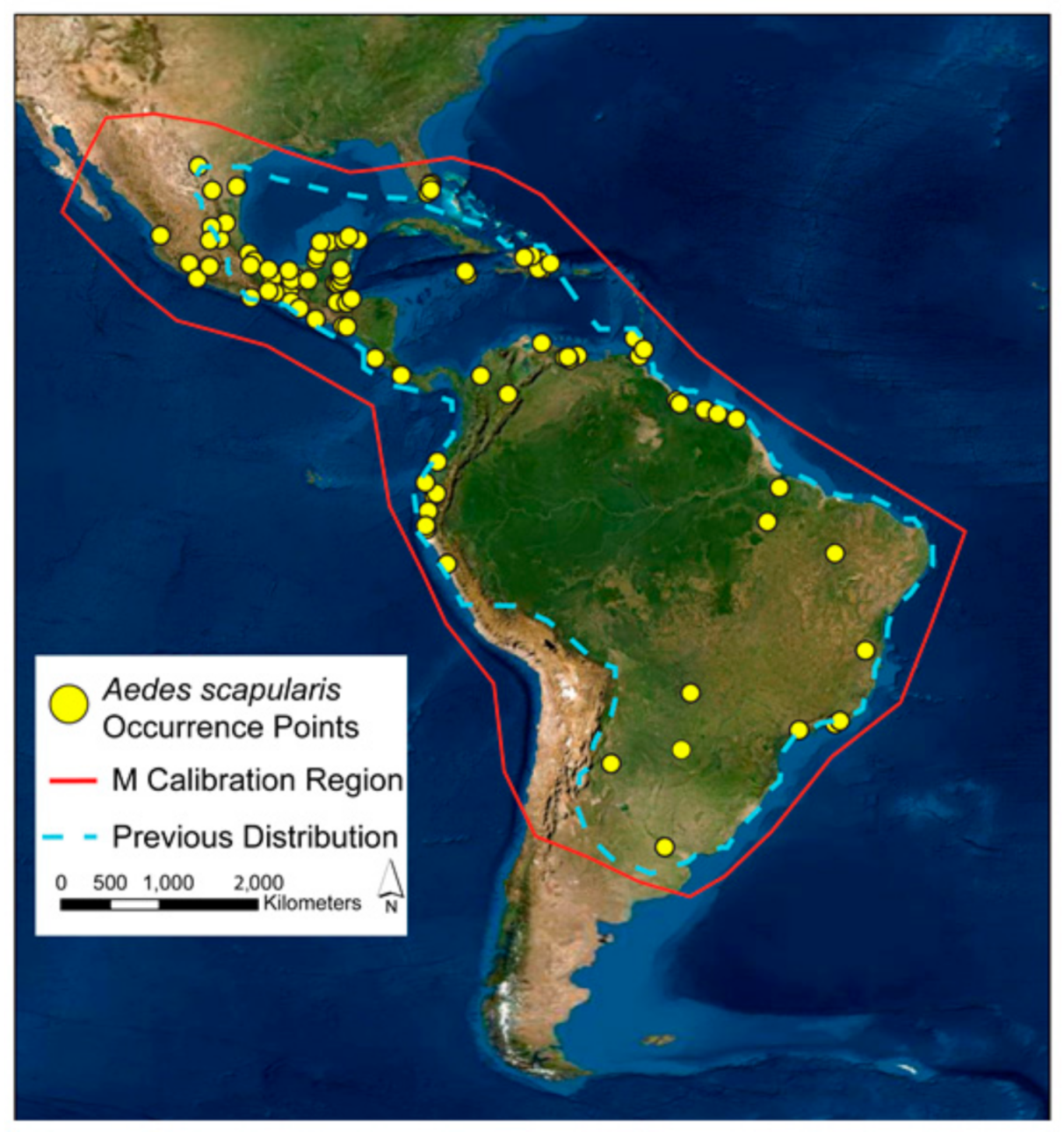
2.1. Calibration Area
2.2. Environmental Data
2.3. Model Calibration
2.4. Model Evaluation
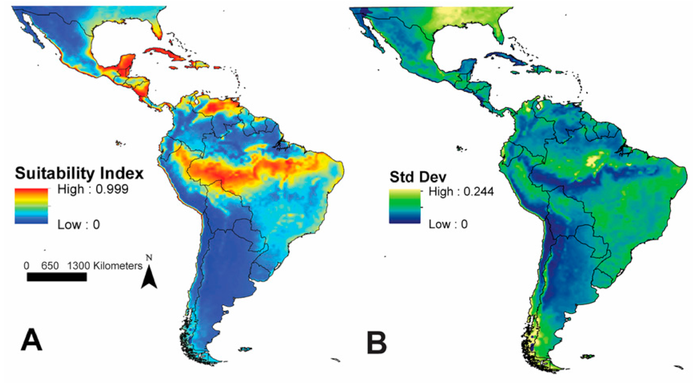
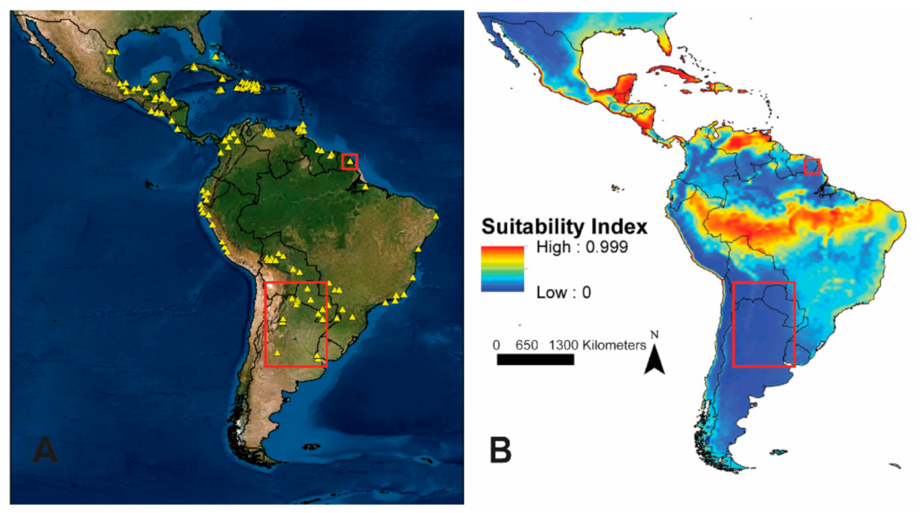
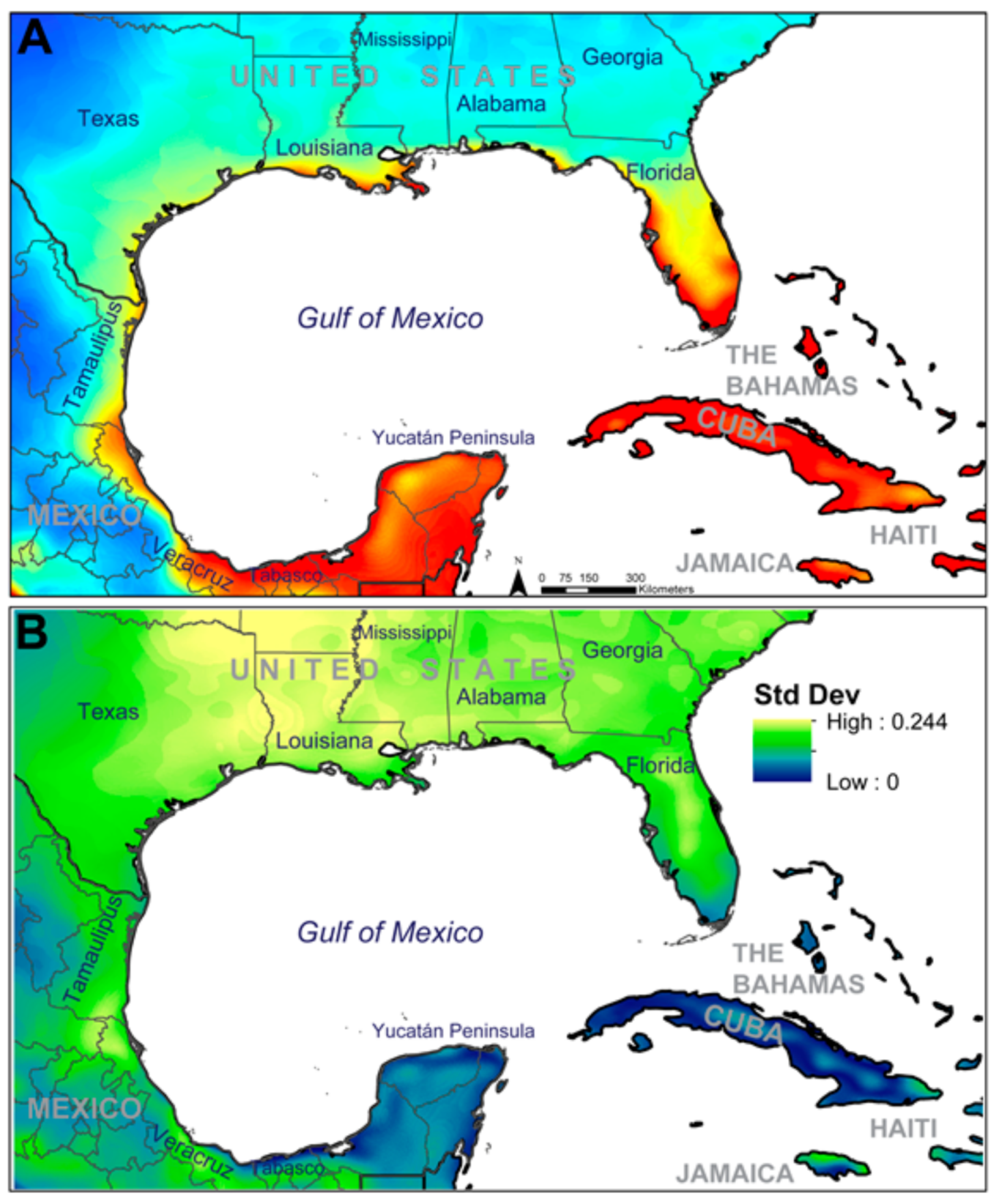
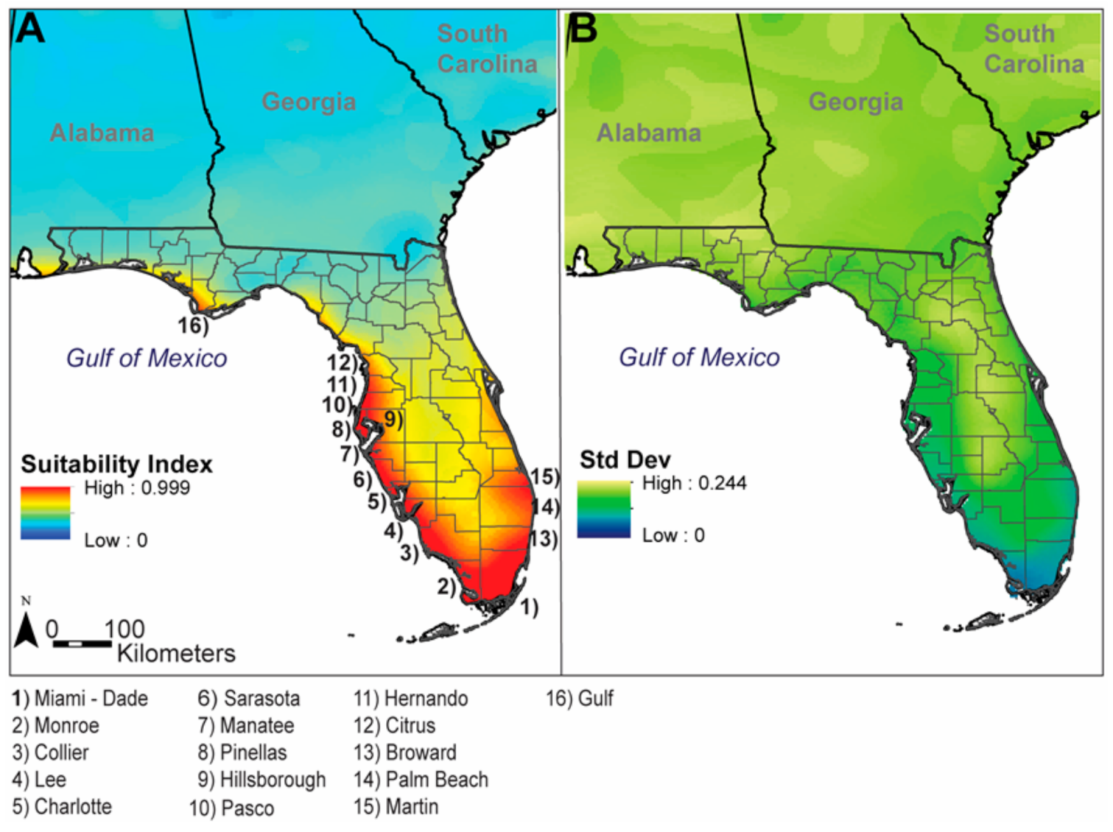
3. Results
4. Discussion
5. Conclusions
Supplementary Materials
Author Contributions
Funding
Data Availability Statement
Conflicts of Interest
References
- Gubler, D.J. Dengue, Urbanization and Globalization: The unholy trinity of the 21(st) Century. Trop. Med. Health 2011, 39, 3–11. [Google Scholar] [CrossRef] [PubMed] [Green Version]
- Reisen, W.K. Landscape epidemiology of vector-borne diseases. Annu. Rev. Entomol. 2010, 55, 461–483. [Google Scholar] [CrossRef] [Green Version]
- Brady, O.J.; Hay, S.I. The global expansion of dengue: How Aedes aegypti mosquitoes enabled the first pandemic arbovirus. Annu. Rev. Entomol. 2020, 65, 191–208. [Google Scholar] [CrossRef] [Green Version]
- Wahid, B.; Ali, A.; Rafique, S.; Idrees, M. Global expansion of chikungunya virus: Mapping the 64-year history. Int. J. Infect. Dis. 2017, 58, 69–76. [Google Scholar] [CrossRef] [PubMed] [Green Version]
- Christofferson, R.C. Zika virus emergence and expansion: Lessons learned from dengue and chikungunya may not provide all the answers. Am. J. Trop. Med. Hyg. 2016, 95, 15–18. [Google Scholar] [CrossRef]
- Reiter, P. Aedes albopictus and the world trade in used tires, 1988–1995: The shape of things to come? J. Am. Mosq. Control. Assoc. 1998, 14, 83–94. [Google Scholar]
- Rochlin, I.; Gaugler, R.; Williges, E.; Farajollahi, A. The rise of the invasives and decline of the natives: Insights revealed from adult populations of container-inhabiting Aedes mosquitoes (Diptera: Culicidae) in temperate North America. Biol. Invasions 2013, 15, 991–1003. [Google Scholar] [CrossRef] [Green Version]
- Connelly, C.R.; Alto, B.W.; O’Meara, G.F. The spread of Culex coronator (Diptera: Culicidae) throughout Florida. J. Vector Ecol. 2016, 41, 195–199. [Google Scholar] [CrossRef] [Green Version]
- Franklinos, L.H.V.; Jones, K.E.; Redding, D.W.; Abubakar, I. The effect of global change on mosquito-borne disease. Lancet Infect. Dis. 2019, 19, e302–e312. [Google Scholar] [CrossRef]
- Lounibos, L.P.; Juliano, S.A. Where Vectors Collide: The importance of mechanisms shaping the realized niche for modeling ranges of invasive Aedes mosquiotes. Biol. Invasions 2018, 20, 1913–1929. [Google Scholar] [CrossRef] [PubMed]
- Juliano, S.A.; Lounibos, L.P. Ecology of invasive mosquitoes: Effects on resident species and on human health. Ecol. Lett. 2005, 8, 558–574. [Google Scholar] [CrossRef] [Green Version]
- Soberón, J.; Nakamura, M. Niches and distributional areas: Concepts, methods, and assumptions. Proc. Natl. Acad. Sci. USA 2009, 106 (Suppl. 2), 19644–19650. [Google Scholar] [CrossRef] [Green Version]
- Chase, J.M.; Leibold, M.A. Ecological Niches: Linking Classical and Contemporary Approaches; University of Chicago Press: Chicago, CA, USA, 2003; p. 212. [Google Scholar]
- Soberon, J.; Peterson, A.T. Interpretation of models of fundamental ecological niches and species‘ distributional areas. Biodivers. Informatics 2005, 2, 1–10. [Google Scholar] [CrossRef] [Green Version]
- Soberón, J. Grinnellian and Eltonian niches and geographic distributions of species. Ecol. Lett. 2007, 10, 1115–1123. [Google Scholar] [CrossRef] [PubMed]
- Wigglesworth, V.B. The Principles of Insect Physiology; Methuen & Co.: London, UK, 1939; pp. 431, 434. [Google Scholar]
- Kraemer, M.U.; Sinka, M.E.; Duda, K.A.; Mylne, A.Q.; Shearer, F.M.; Barker, C.M.; Moore, C.G.; Carvalho, R.G.; Coelho, G.E.; Van Bortel, W.; et al. The global distribution of the arbovirus vectors Aedes aegypti and Ae. albopictus. Elife 2015, 4, e08347. [Google Scholar] [CrossRef]
- Campbell, L.P.; Luther, C.; Moo-Llanes, D.; Ramsey, J.M.; Danis-Lozano, R.; Peterson, A.T. Climate change influences on global distributions of dengue and chikungunya virus vectors. Philos. Trans. R. Soc. Lond. B Biol. Sci. 2015, 370. [Google Scholar] [CrossRef] [PubMed]
- Mordecai, E.A.; Ryan, S.J.; Caldwell, J.M.; Shah, M.M.; LaBeaud, A.D. Climate change could shift disease burden from malaria to arboviruses in Africa. Lancet Planet. Health 2020, 4, e416–e423. [Google Scholar] [CrossRef]
- Ryan, S.J.; Carlson, C.J.; Mordecai, E.A.; Johnson, L.R. Global expansion and redistribution of Aedes-borne virus transmission risk with climate change. PLoS Negl. Trop. Dis. 2019, 13, e0007213. [Google Scholar] [CrossRef] [Green Version]
- Peterson, A.T.; Campbell, L.P.; Moo-Llanes, D.A.; Travi, B.; González, C.; Ferro, M.C.; Ferreira, G.E.M.; Brandão-Filho, S.P.; Cupolillo, E.; Ramsey, J.; et al. Influences of climate change on the potential distribution of Lutzomyia longipalpis sensu lato (Psychodidae: Phlebotominae). Int. J. Parasitol. 2017, 47, 667–674. [Google Scholar] [CrossRef]
- Peach, D.A.H.; Almond, M.; Pol, J.C. Modeled distributions of Aedes japonicus japonicus and Aedes togoi (Diptera: Culicidae) in the United States, Canada, and northern Latin America. J. Vector Ecol. 2019, 44, 119–129. [Google Scholar] [CrossRef] [Green Version]
- Griffith, G.; Omernik, J. Ecoregions of Florida (EPA); Environmental Information Coalition, National Council for Science and the Environment: Washington, DC, USA, 2008. [Google Scholar]
- Wilke, A.B.B.; Benelli, G.; Beier, J.C. Beyond frontiers: On invasive alien mosquito species in America and Europe. PLoS Negl. Trop. Dis. 2020, 14, e0007864. [Google Scholar] [CrossRef]
- Reeves, L.; Medina, J.; Miqueli, E.; Sloyer, K.; Petrie, W.; Vasquez, C.; Burkett-Cadena, N. Establishment of Aedes (Ochlerotatus) scapularis (Diptera: Culicidae) in Mainland Florida, with Notes on the Ochlerotatus Group in the United States. J. Med. Entomol. 2020, tjaa250. [Google Scholar] [CrossRef]
- Arnell, J. Mosquito studies (Diptera, Culicidae) XXXIII. A revision of the scapularis group of Aedes. Contrib. Am. Entomol. Inst. 1976, 13, 1–144. [Google Scholar]
- Shannon, R.C.; Whitman, L.; Franca, M. Yellow fever virus in jungle mosquitoes. Science 1938, 88, 110–111. [Google Scholar] [CrossRef] [PubMed]
- Mitchell, C.J.; Forattini, O.P.; Miller, B.R. Vector competence experiments with Rocio virus and three mosquito species from the epidemic zone in Brazil. Rev. Saude Publica 1986, 20, 171–177. [Google Scholar] [CrossRef]
- Aitken, T.H.; Anderson, C.R. Virus transmission studies with Trinidadian mosquitoes II. Further observations. Am. J. Trop. Med. Hyg. 1959, 8, 41–45. [Google Scholar] [CrossRef] [PubMed]
- Pauvolid-Corrêa, A.; Kenney, J.L.; Couto-Lima, D.; Campos, Z.M.; Schatzmayr, H.G.; Nogueira, R.M.; Brault, A.C.; Komar, N. Ilheus virus isolation in the Pantanal, west-central Brazil. PLoS Negl. Trop. Dis. 2013, 7, e2318. [Google Scholar] [CrossRef] [PubMed] [Green Version]
- Causey, O.; Causey, C.; Maroja, O.; Macedo, D. The isolation of arthropod-borne viruses, including members of two hitherto undescribed serological groups, in the Amazon region of Brazil. Am. J. Trop. Med. Hyg. 1961, 10, 227–249. [Google Scholar] [CrossRef]
- Sellers, R.; Bergold, G.; Suarez, O.; Morales, A. Investigations during Venezuelan equine encephalitis outbreaks in Venezuela—1962–1964. Am. J. Trop. Med. Hyg. 1965, 14, 460–469. [Google Scholar] [CrossRef]
- Scherer, W.F.; Dickerman, R.W.; Diaz-Najera, A.; Ward, B.A.; Miller, M.H.; Schaffer, P.A. Ecologic studies of Venezuelan encephalitis virus in southeastern México III. Infection of mosquitoes. Am. J. Trop. Med. Hyg. 1971, 20, 969–979. [Google Scholar] [CrossRef]
- Sudia, W.D.; Newhouse, V.F. Epidemic Venezuelan equine encephalitis in North America: A summary of virus-vector-host relationships. Am. J. Epidemiol. 1975, 101, 1–13. [Google Scholar] [CrossRef]
- Méndez-López, M.R.; Attoui, H.; Florin, D.; Calisher, C.H.; Florian-Carrillo, J.C.; Montero, S. Association of vectors and environmental conditions during the emergence of Peruvian horse sickness orbivirus and Yunnan orbivirus in northern Peru. J. Vector Ecol. 2015, 40, 355–363. [Google Scholar] [CrossRef] [PubMed]
- Lourenço-de-Oliveira, R.; Deane, L. Presumed Dirofilaria immitis infections in wild-caught Aedes taeniorhynchus and Aedes scapularis in Rio de Janeiro, Brazil. Memórias do Instituto Oswaldo Cruz 1995, 90, 387–388. [Google Scholar] [CrossRef]
- Rachou, E.; Lima, M.; Neto, J.; Martins, C. Aëdes scapularis, a new proved vector of W. bancroftii in southern Brazil. Revista Brasileira de Malariologia e Doenças Tropicais 1954, 6, 145. [Google Scholar]
- Forattini, O.; de Castro Gomes, A.; Natal, D.; Kakitani, I.; Marucci, D. Preferências alimentares de mosquitos Culicidae no Vale do Ribeira, São Paulo, Brasil. Revista de Saúde Pública 1987, 21, 171–187. [Google Scholar] [CrossRef] [PubMed] [Green Version]
- Forattini, O.; de Castro Gomes, A.; Natal, D.; Kakitani, I.; Marucci, D. Preferências alimentares e domiciliação de mosquitos Culicidae no Vale do Ribeira, São Paulo, Brasil, com especial referência a Aedes scapularis e a Culex(Melanoconion). Revista de Saúde Pública 1989, 23, 9–19. [Google Scholar] [CrossRef] [PubMed]
- Gomes, A.; Silva, N.; Marques, G.; Brito, M. Host-feeding patterns of potential human disease vectors in the Paraíba Valley Region, State of São Paulo, Brazil. J. Vector Ecol. 2003, 28, 74–78. [Google Scholar]
- Loroso, E.; Faria, M.; De Oliveira, L.; Alencar, J.; Marcondes, C. Blood meal identification of selected mosquitoes in Rio de Janeiro, Brazil. J. Am. Mosq. Contr. 2010, 26, 18–23. [Google Scholar] [CrossRef] [PubMed]
- De Carvalho, G.C.; Malafronte, R.o.S.; Miti Izumisawa, C.; Souza Teixeira, R.; Natal, L.; Marrelli, M.T. Blood meal sources of mosquitoes captured in municipal parks in São Paulo, Brazil. J. Vector Ecol. 2014, 39, 146–152. [Google Scholar] [CrossRef] [PubMed] [Green Version]
- Alencar, J.; Mello, C.F.; Gil-Santana, H.R.; Giupponi, A.P.; Araújo, A.N.; Lorosa, E.S.; Guimarães, A.; Silva, J.o.S. Feeding Patterns of Mosquitoes (Diptera: Culicidae) in the Atlantic Forest, Rio de Janeiro, Brazil. J. Med. Entomol. 2015, 52, 783–788. [Google Scholar] [CrossRef] [PubMed]
- Mucci, L.F.; Júnior, R.P.; de Paula, M.B.; Scandar, S.A.; Pacchioni, M.L.; Fernandes, A.; Consales, C.A. Feeding habits of mosquitoes (Diptera: Culicidae) in an area of sylvatic transmission of yellow fever in the state of São Paulo, Brazil. J. Venom. Anim. Toxins Incl. Trop. Dis. 2015, 21, 6. [Google Scholar] [CrossRef] [Green Version]
- Santos, C.S.; Pie, M.R.; da Rocha, T.C.; Navarro-Silva, M.A. Molecular identification of blood meals in mosquitoes (Diptera, Culicidae) in urban and forested habitats in southern Brazil. PLoS ONE 2019, 14, e0212517. [Google Scholar] [CrossRef]
- Klein, T.; Lima, J.; Tang, A. Seasonal distribution and diel biting patterns of culicine mosquitoes in Costa Marques, Rondônia, Brazil. Memórias do Instituto Oswaldo Cruz 1992, 87, 141–148. [Google Scholar] [CrossRef] [PubMed]
- Forattini, O.P.; Kakitani, I.; Massad, E.; Marucci, D. Studies on mosquitoes (Diptera: Culicidae) and anthropic environment. 9-Synanthropy and epidemiological vector role of Aedes scapularis in south-eastern Brazil. Rev. Saude Publica 1995, 29, 199–207. [Google Scholar] [CrossRef] [PubMed] [Green Version]
- Causey, O.; Kumm, H. Dispersion of forest mosquitoes in Brazil; preliminary studies. Am. J. Trop. Med. Hyg. 1948, 28, 469–480. [Google Scholar] [CrossRef] [PubMed]
- Peterson, A.T. Ecological Niches and Geographic Distributions; Princeton University Press: Princeton, NJ, USA, 2011; p. 314. [Google Scholar]
- Peterson, A.T. Mapping Disease Transmission Risk: Enriching Models Using Biogeography and Ecology; Johns Hopkins University Press: Baltimore, MD, USA, 2014; p. 210. [Google Scholar]
- Osorio-Olvera, L.; Lira-Noriega, A.; Soberón, J.; Townsend Peterson, A.; Falconi, M.; Contreras-Díaz, R.; Martínez-Meyer, E.; Barve, V.; Barve, N. ntbox: An R package with graphical user interface for modeling and evaluating multidimensional ecological niches. Methods Ecol. Evol. 2020, 11, 1199–1206. [Google Scholar] [CrossRef]
- Boria, R.; Olson, L.; Goodman, S.; Anderson, R. Spatial filtering to reduce sampling bias can improve the performance of ecological niche models. Ecol. Model. 2014, 275, 73–77. [Google Scholar] [CrossRef]
- Varela, S.; Anderson, R.; García-Valdés, R.; Fernández-González, F. Environmental filters reduce the effects of sampling bias and improve predictions of ecological niche models. Ecography 2014, 37, 1084–1091. [Google Scholar] [CrossRef]
- Barve, N.; Barve, V.; Jímenez-Valverde, A.; Lira-Noriega, A.; Maher, S.P.; Peterson, A.T.; Soberon, J.; Villalobos, F. The crucial role of the accessible area in ecological niche modeling and species distribution modeling. Ecol. Model. 2011, 222, 1810–1819. [Google Scholar] [CrossRef]
- Capinha, C.; Pateiro-López, B. Predicting species distributions in new areas or time periods using alpha-shapes. Ecol. Inform. 2014, 24, 231–237. [Google Scholar] [CrossRef]
- Kottek, M.; Grieser, J.; Beck, C.; Rudolf, B.; Rubel, F. World map of the Köppen-Geiger climate classification updated. Meteorologische Zeitschrift 2006, 15, 259–263. [Google Scholar] [CrossRef]
- Vega, C.G.; Pertierra, L.R.; Olalla-Tarraga, M.A. MERRAclim, a high-resolution global dataset of remotely sensed bioclimatic variables for ecological modelling. Sci. Data 2017, 4, 170078. [Google Scholar] [CrossRef] [PubMed] [Green Version]
- Hijmans, R. Raster: Geographic Data Analysis and Modeling. R Package Version 2.5-2. 2015. Available online: https://CRAN.R-project.org/package=raster (accessed on 20 October 2020).
- Merow, C.; Smith, M.J.; Silander, J.A. A practical guide to Maxent for modeling species’ distributions: What it does, and why inputs and settings matter. Ecography 2013, 36, 1058–1069. [Google Scholar] [CrossRef]
- Phillips, S.; Dudik, S.; Shapire, R. Maxent Software for Modeling Species Niches and Distributions. Version 3.4.1. Available online: http://biodiversityinformatics.amnh.org/open_source/maxent/ (accessed on 6 October 2020).
- Cobos, M.; Peterson, A.; Barve, N.; Osorio-Olvera, L. kuenm: An R package for detailed development of ecological niche models using Maxent. PEERJ 2019, 7. [Google Scholar] [CrossRef] [PubMed] [Green Version]
- Warren, D.L.; Seifert, S.N. Ecological niche modeling in Maxent: The importance of model complexity and the performance of model selection criteria. Ecol. Appl. 2011, 21, 335–342. [Google Scholar] [CrossRef] [Green Version]
- Phillips, S.J.; Anderson, R.P.; Dudik, M.; Schapire, R.E.; Blair, M.E. Opening the black box: An open-source release of Maxent. Ecography 2017, 40, 887–893. [Google Scholar] [CrossRef]
- Phillips, S.J.; Anderson, R.; Schapire, R.E. Maximum entropy modeling of species geographic distributions. Ecol. Model. 2006, 190, 231–259. [Google Scholar] [CrossRef] [Green Version]
- Syfert, M.M.; Smith, M.J.; Coomes, D.A. The effects of sampling bias and model complexity on the predictive performance of MaxEnt species distribution models. PLoS ONE 2013, 8, e55158. [Google Scholar] [CrossRef]
- Phillips, S.; Dudík, M. Modeling of species distributions with Maxent: New extensions and a comprehensive evaluation. Ecography 2008, 31, 161–175. [Google Scholar] [CrossRef]
- Peterson, A.T.; Papeş, M.; Soberón, J. Rethinking receiver operating characteristic analysis applications in ecological niche modeling. Ecol. Model. 2008, 213, 63–72. [Google Scholar] [CrossRef]
- Elith, J.; Phillips, S.; Hastie, T.; Dudik, M.; Chee, Y.; Yates, C. A statistical explanation of MaxEnt for ecologists. Divers. Distrib. 2011, 17, 43–57. [Google Scholar] [CrossRef]
- Arbogast, A.F. Discovering Physical Geography, 2nd ed.; John Wiley & Sons: Hoboken, NJ, USA, 2011; p. 639. [Google Scholar]
- Mitchell, C.; Darsie, R. Mosquitoes of Argentina Part II: Geographic distribution and bibliography. Mosq. Syst. 1985, 17, 279–360. [Google Scholar]
- Darsie, R.F.; Shroyer, D.A. Culex (Culex) declarator, a mosquito species new to Florida. J. Am. Mosq. Control. Assoc. 2004, 20, 224–227. [Google Scholar] [PubMed]
- Shin, D.; O’Meara, G.F.; Civana, A.; Shroyer, D.A.; Miqueli, E. Culex interrogator (Diptera: Culicidae), a mosquito species new to Florida. J. Vector Ecol. 2016, 41, 316–319. [Google Scholar] [CrossRef] [PubMed]
- Lloyd, A.M.; Connelly, C.R.; Carlson, D.B. (Eds.) Florida Coordinating Council on Mosquito Control. In Florida Mosquito Control: The State of the Mission as Defined by Mosquito Controllers, Regulators, and Environmental Managers; University of Florida, Institute of Food and Agricultural Sciences, Florida Medical Entomology Laboratory: Vero Beach, FL, USA, 2018. [Google Scholar]
- Darsie, R.; Morris, C. Keys to the Adult Females and Fourth Instar Larvae of the Mosquitoes of Florida (Diptera, Culicidae); Florida Mosquito Control Association: Fort Myers, FL, USA, 2003. [Google Scholar]


| Variable Number | Variable Name |
|---|---|
| Bio1 | Average Annual Temperature |
| Bio3 | Average Isothermality (mean diurnal range/temperature annual range) |
| Bio5 | Average Maximum Temperature of the Warmest Month |
| Bio6 | Average Minimum Temperature of the Coldest Month |
| Bio12 | Average Annual Specific Humidity |
| Bio16 | Average Specific Humidity of the Wettest Quarter |
| Bio17 | Average Specific Humidity of the Driest Quarter |
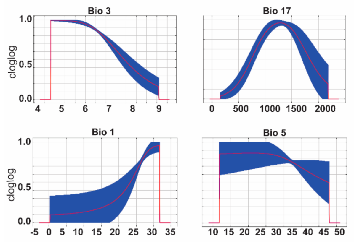
| Variable | Variable Description | Percent Contribution |
|---|---|---|
| Bio3 | Average Isothermality (mean diurnal range/temperature annual range) | 48.6 |
| Bio17 | Average Specific Humidity of the Driest Quarter | 22.3 |
| Bio1 | Average Annual Temperature | 15.6 |
| Bio5 | Average Maximum Temperature of the Warmest Month | 13.5 |
Publisher’s Note: MDPI stays neutral with regard to jurisdictional claims in published maps and institutional affiliations. |
© 2021 by the authors. Licensee MDPI, Basel, Switzerland. This article is an open access article distributed under the terms and conditions of the Creative Commons Attribution (CC BY) license (http://creativecommons.org/licenses/by/4.0/).
Share and Cite
Campbell, L.P.; Burkett-Cadena, N.D.; Miqueli, E.; Unlu, I.; Sloyer, K.E.; Medina, J.; Vasquez, C.; Petrie, W.; Reeves, L.E. Potential Distribution of Aedes (Ochlerotatus) scapularis (Diptera: Culicidae): A Vector Mosquito New to the Florida Peninsula. Insects 2021, 12, 213. https://0-doi-org.brum.beds.ac.uk/10.3390/insects12030213
Campbell LP, Burkett-Cadena ND, Miqueli E, Unlu I, Sloyer KE, Medina J, Vasquez C, Petrie W, Reeves LE. Potential Distribution of Aedes (Ochlerotatus) scapularis (Diptera: Culicidae): A Vector Mosquito New to the Florida Peninsula. Insects. 2021; 12(3):213. https://0-doi-org.brum.beds.ac.uk/10.3390/insects12030213
Chicago/Turabian StyleCampbell, Lindsay P., Nathan D. Burkett-Cadena, Evaristo Miqueli, Isik Unlu, Kristin E. Sloyer, Johana Medina, Chalmers Vasquez, William Petrie, and Lawrence E. Reeves. 2021. "Potential Distribution of Aedes (Ochlerotatus) scapularis (Diptera: Culicidae): A Vector Mosquito New to the Florida Peninsula" Insects 12, no. 3: 213. https://0-doi-org.brum.beds.ac.uk/10.3390/insects12030213