Article

Polyethylene Identification in Ocean Water Samples by Means of 50 keV Energy Electron Beam

1
Biology Department, Truckee Meadow Community College, Reno, Nevada, NV 89512-3999, USA
2
Particle Physics Department, BabuHawaii Foundation, Honolulu, HI 96811, USA
*
Authors to whom correspondence should be addressed.
Submission received: 16 September 2020 / Revised: 21 October 2020 / Accepted: 21 October 2020 / Published: 31 October 2020

Abstract

:
This study presents a new methodology to reveal traces of polyethylene (the most common microplastic particles, known as a structure of C2H4) in a sample of ocean water by the irradiation of a 50 keV, 1 µA electron beam. This is performed by analyzing the photon (produced by the electrons in water) fluxes and spectra (i.e., fluxes as a function of photon energy) with different types of contaminated water using an adequate device and in particular looking at the peculiar interactions of electrons/photons with the potential abnormal atomic hydrogen (H), oxygen (O), carbon (C), and phosphorus (P) compositions present in the water, as a function of living and nonliving organic organisms with PO4 group RNA/DNA strands in a cluster configuration through a volumetric cells grid.

Graphical Abstract

1. Introduction

Plastic is the most common type of marine debris found in oceans, and it is the most widespread problem affecting the marine environment. It also threatens ocean health, food safety and quality, human health, and coastal tourism, and it contributes to climate change [1,2,3,4,5]. Plastic debris can come in many different shapes and sizes, but those that are less than five millimeters across (or the size of a sesame seed) are called “microplastics”. One of the most common microplastics in use today is polyethylene, with most of the known kinds having the chemical formula (C2H4)n. It is a linear, man-made homopolymer primarily used for packaging (plastic bags, plastic films, geomembranes, containers including bottles, etc.). As of 2019, over 100 million tons of polyethylene resins are being produced annually, accounting for 34% of the total plastics market.
This is an emerging field of study, and not much is known yet about microplastics and their impact on the environment. The NOAA Marine Debris Program is pursuing efforts within the NOAA to research this important topic.
Different standardized field methods have been developed for the collection of microplastic samples in sediment [6,7,8,9,10,11,12,13], sand, and surface water, all of which continue to be tested. In the end, the field and laboratory protocols will allow for a global comparison of the quantity of microplastics released into the environment, which is the first step in determining the final distribution, impacts, and fate of these debris.
Microplastics come from a variety of sources, including larger plastic debris that degrade into smaller and smaller pieces. In addition, microspheres, a type of microplastic, are tiny particle pieces of plastic polyethylene that are added as exfoliators to health and beauty products, such as some detergents and toothpastes, passing easily through water filtration systems, thus posing a threat to aquatic life.
The most visible impacts of marine plastics are the ingestion, suffocation, and entanglement of hundreds of marine species. Marine wildlife such as seabirds, whales, fish, and turtles, mistake plastic waste for prey, and most die of starvation as their stomachs are filled with plastic debris. They also suffer from lacerations, infections, reduced ability to swim, and internal injuries. Floating plastics also contribute to the spread of invasive marine organisms and bacteria, which disrupt ecosystems. Plastic degrades (i.e., breaks down into pieces), but it does not biodegrade (break down through natural decomposition). This has become a problem over time, as all the plastic pieces that have been generated over the last seven decades have steadily increased their presence as a contaminant, creating a biological alteration. According to the United Nations Environment Program, these plastic microspheres first appeared in personal care products about fifty years ago, with plastic replacing more and more natural ingredients. Until 2012, this problem was still relatively unknown, with an abundance of products containing plastic microspheres on the market and leading now to an increase in microplastic detection and identification demand.
Ocean water also contains microorganisms, live matter and not, such as viruses, bacteria, and microorganisms like plankton with a different PO4 phosphorus content [14,15,16,17,18,19,20,21,22,23,24,25,26,27,28,29]. Viruses, for example, are intracellular parasites composed of a nucleic acid surrounded by a protein coat, the capsid. Some viruses contain a lipid envelope, derived from the host, surrounding the capsid. The nucleic acid found in viruses can consist of either RNA or DNA. RNA is composed of nucleotides, each containing a sugar (deoxyribose), a nitrogen-containing base (adenine, uracil, guanine, and cytosine), and a phosphate group PO4. Members of the Coronoviridae family measure 80–160 nm in diameter. Generally, there are 1–10 million viruses and about 100,000 to 1 million bacteria cells for each milliliter of ocean water.
The proposed methodology is based on a subatomic particle analysis and the subsequent detection of particles, and the aim is to use this to identify polyethylene particles in the water among microorganisms. It could be an interesting research approach for the ocean studies field and for the food and beverage industries field in order to detect microplastic contamination in their products. This type of approach would make it easier to test water samples and analyze data in real time in comparison to other state-of-the-art detection processes, and it also allows test procedures to be conducted for quality assurance in the food and beverage industries with simple hardware.

2. Materials and Methods

The physical model under analysis and its simulation by the MCNPX Monte Carlo simulation subatomic particles code [30,31,32] are based on an electron beam source of 50 keV and 1 µA, easily accessible from an extraction line of an industrial linear/circular particle accelerator, interacting with the water sample target. The beam energy and current are based on cross section considerations and radiation requirements; the beam interacts with a cylindrical sample volume—with the axis on x—of ocean water of radius r = 5 cm and height h = 10 cm as s sample tank (Figure 1), which is analyzed at x = 10 cm through a double plates ionization chamber detector.
The ocean water taken into account was chemically analyzed, as shown in Table 1 [12].
Among the all possible subatomic particles generated, only photons (coming from electron coherent and incoherent scattering, absorption, knock on, decay, fluorescence, bremsstrahlung, and photoelectric effect) were taken into account, as reported in Table 2 (where the percent contribution of different phenomena which create photons are shown) and Table 3 (where the percent contribution of different elements to the production of photons are shown), as the other ones are actually negligible. As for Table 2, the photoelectric effect consists of the absorption of the incident photon energy E, with emission of several fluorescent photons and the ejection or excitation of an orbital electron of binding energy e < E. Photons of first fluorescence are emitted with energy greater than 1 keV; those of second fluorescence are still greater than 1 keV and are caused by residual excitation of the first fluorescence process, leading to a second emission.
It has to be underlined that the MCNPX analysis took into account both electrons and photons without neglecting any secondary photon production by performing a photon/electron coupled calculation and by keeping track of the electron mean free path in the water sample, which is around 5060 nm due to multiple volume cells of the electron mean path magnitude. All the results proposed concern the photon fluxes and spectra of interest, where all the possible primary and secondary electron productions (mode e, p) into the sample volume were taken into account.
The polyethylene particles are described in 11 cluster configurations (Table 4) through a highly sophisticated volumetric cell grid (Figure 2 and Figure 3); each cluster is composed of microspheres with a radius of 0.1 mm and a volume of 4 × 10¹⁹ − 3 mm3 per particle, with a mutual distance of 1–9 cm among the clusters along all the axes (Figure 3) and evaluated on an atomic fraction of C, H in the ocean water sample tank at different concentrations from 10 ppm up to 10,000 ppm (Table 5, Table 6, Table 7 and Table 8).
It must be underlined that a benchmark model was also taken into consideration in order to evaluate a potential enrichment in microorganisms, bacteria, and viruses, which can alter mainly the carbonium and in particular the phosphorus PO4 group analysis outcome; these all were analyzed on multiple “tallies” (control check volumes/surfaces) in order to evaluate energy distributions and particle mean free path (yellow squares, Figure 4). In order to do that, in the benchmark, a 100-ppm polyethylene content in the ocean water sample in the cluster configuration was kept constant, and different enriched mixture scenarios at 0.7 ppm, 7 ppm, 70 ppm, and 700 ppm of potential living/nonliving matter and microorganisms were studied, adjusting their own contributions in the final solution in terms of atomic C, H, O, P content and the result in terms of particle spectra and fluxes.
MCNPX was performed chronologically in different cluster stages: Stage 1, with 0 ppm contamination to investigate the physics involved in the basic case; Stage 2, evaluating an escalating contamination grade as maximum stress test of 10 ppm, 100 ppm, 1000 ppm, and 10,000 ppm (Table 9 and Table 10), just as a benchmark to determine the subatomic particles’ stopping power and the shielding effects that give the photon fluxes and energy spectra, due to all the experimental cross sections involved in these cases (Figure 5, Figure 6, Figure 7, Figure 8, Figure 9, Figure 10, Figure 11, Figure 12, Figure 13, Figure 14, Figure 15, Figure 16, Figure 17, Figure 18, Figure 19, Figure 20, Figure 21, Figure 22, Figure 23 and Figure 24). The MCNPX code by various variance reduction techniques fulfils 10 statistical tests [30] with an average relative error of 2%.

3. Results

This section presents the results of the analysis showing the photon fluxes and energy spectra of the Monte Carlo simulations in the presence of polyethylene contaminations and also without it in the detector chamber, located at x = 10 cm on the top of the sample tank on the x-axis.
The study analyzed the photon fluxes and their contributions on three discrete energy bins: 30, 40, and 50 keV at different polyethylene grades with an energy spectrum peak located at 40 keV. The reason of a 40 keV peak can be explained by the cross section considerations and energy spectrum degradation. As shown in Figure 21, the total photon cross section value (in barns) decreases as a function of the energy from 8 barns at 40 keV to 3 barns at 50 keV. Moreover, the detection surface is located at x = 10 cm after the primary injection beam at x = 0 cm, leading to the detection of a particle flux and spectrum in a different energy configuration due to scattering, fluorescence, absorption, and photoelectric effect, which are responsible for leaving an intact high energy photon band after x = 5 cm and thus made negligible the energy contribution for the low band spectrum E < 20 keV. Between the interval 5 < x < 10 cm, the photon flux, present in a high energy band configuration, interacts with the nonhomogeneous media due to scattering, fluorescence, absorption, and photoelectric effect, thus causing a degradation of the 50 keV energy bin and leading to an average value of 40 keV.
As shown in Figure 25 and Figure 26, the total photon flux and each flux that was evaluated on 30, 40, and 50 keV, increase between 0–10 ppm of 1.4% due to electron bremsstrahlung and photelectric-fluorescence on polyethylene particles. However, it has to be underlined that in the beginning of the contamination process, the main atomic element present in the water is oxygen with a weight percentage of 85.70%, and its photon cross sections (Figure 10, Figure 11, Figure 12, Figure 13 and Figure 14) show a higher value (in barn unities) compared to the carbon ones (Figure 5, Figure 6, Figure 7, Figure 8 and Figure 9). These cross-section considerations are the main reason to understand the decrease of 5.6% between 10–100 ppm where the amount of oxygen reduces while the amount of carbon increases but with a less effective cross-section value. However, after 100 ppm, due to the electron stopping power and the bremsstrahlung/photoelectric process on the mixture, the photon flux trend starts to increase 10% up to 1000 ppm and of 50.7% from 1000–10,000 ppm.
Figure 25, Figure 26, Figure 27, Figure 28 and Figure 29 show the fluxes and photon energy spectra and the different behaviors as a function of polyethylene contamination on 3 discrete energy bins.
As mentioned in Section 2, the graphs in Figure 30, Figure 31, Figure 32 and Figure 33 show the photon fluxes and energy spectra as well as the different behaviors of fixed contamination test case of 100 ppm polyethylene, in cluster configuration, and mixed as a function of microorganism group PO4, evaluated on 3 discrete energy bins, i.e., 30, 40, and 50 keV.

4. Discussion

The photon fluxes and spectra can discriminate the amount of polyethylene contamination by using to its own “particle signature” in terms of photon flux at the detector point combined with the spectrum analysis, as reported for 30, 40, and 50 keV.
As shown in Figure 27, Figure 28 and Figure 29, the photon flux associated with the sample of ocean water at different concentrations of the polyethylene shows both a trend in term of photon/s*cm2 and differences from an energy spectrum point of view to evaluate its own contributions in counting the number of photons on each energy line:
  • The 10-ppm polyethylene case can be discriminated using the photon flux counts at the detector evaluated on the 30 and 40 keV spectra compared to the standard ocean water.
  • The 100-ppm polyethylene case can be discriminated using the photon flux counts at the detector and the 30, 40, and 50 keV spectra compared to the 10 ppm one.
  • The 1000-ppm polyethylene case can be discriminated using the photon flux counts at the detector and the 30, 40, and 50 keV spectra compared to the 100 ppm one.
  • The 10,000-ppm polyethylene case can be discriminated using the photon flux counts at the detector and the 30, 40, and 50 keV spectra compared to the 1000 ppm one.
As shown in Figure 30, the photon flux, starting from the ocean water plus 100 ppm polyethylene contamination, increases as a function of the ppm amount of microorganisms added in the water sample tank. This behavior is due to an increase from 0.7 ppm to 700 ppm of P (present in the PO4 group in the sample) and also due to a change subsequently in the cross-section value, thus affecting the photon population (Figure 15, Figure 16, Figure 17 and Figure 18). In the presence of microorganism living/nonliving matter, the photon flux shows, taking a parametric comparison case of 100 ppm polyethylene, an increase of 2.3% from 0 to 0.7 ppm of microorganisms, 0.2% from 0.7 to 7 ppm of microorganisms, 0.7% from 7 to 70 ppm of microorganisms, and a decrease of 1% from 70 to 700 ppm of microorganisms. Furthermore, it has to be underlined that even if there is a significant change in the total photon population counts, what has been one of the research main goals was to discriminate the number of microorganisms present in the sample tank through a spectrum analysis and relative photon flux counts on the 3 energy bins.
As shown, the photon flux associated with the 100-ppm polyethylene at different concentrations of microorganisms increases in terms of photon/s*cm2, and differences appear in the contribution to the total by different energy photons (Figure 31, Figure 32 and Figure 33):
5.
The 0.7-ppm microorganisms case can be discriminated using the photon flux counts at the detector evaluated on the 30 and 50 keV spectrum lines compared to the ocean water + 100 ppm polyethylene combination at the same energy conditions.
6.
The 7-ppm microorganisms case can be discriminated using the photon flux counts at the detector evaluated on the 50 keV spectrum line compared to the ocean water + 100 ppm polyethylene + 0.7 ppm microorganisms combination at the same energy condition.
7.
The 70-ppm microorganisms case can be discriminated using the photon flux counts at the detector evaluated on the 40 and 50 keV spectrum lines compared to the ocean water + 100 ppm polyethylene + 7 ppm microorganisms combination at the same energy conditions.
8.
The 700-ppm microorganisms case can be discriminated using the photon flux counts at the detector evaluated on the 40 and 50 keV spectrum lines compared to the ocean water + 100 ppm polyethylene + 70 ppm microorganisms combination at the same energy conditions.

5. Conclusions

This study proposed a new approach to identify low contaminations of polyethylene mixed in water using a Monte Carlo simulation performed by the MCNPX subatomic particles code and evaluating the secondary photon (generated by an electron beam of 50 keV and 1 µA) energy spectra and fluxes revealed by an adequate detector.
Different types of contamination grades can be discriminated using their trend Vs photon/s*cm2 evaluated on at least three energy bins, which in this case are 30, 40, and 50 keV. Every single contamination is unique in its own spectrum photon signature, and the flux acts as a unique identifier in the detection process so that, in combination with the microorganisms analysis, it can give the ppm amount of polyethylene in ocean water, drinking/non-drinking water, and food/beverage processing.

Author Contributions

Conceptualization, L.J.T. and P.N.; methodology, L.J.T., P.N. and J.I.A.; software, L.J.T., P.N.; validation, E.M. and J.I.A.; investigation, E.M., D.C.; data curation, R.S.; writing—original draft preparation, P.N., D.C.; writing—review and editing, L.J.T., P.N., J.I.A.; visualization, R.S.; All authors have read and agreed to the published version of the manuscript.
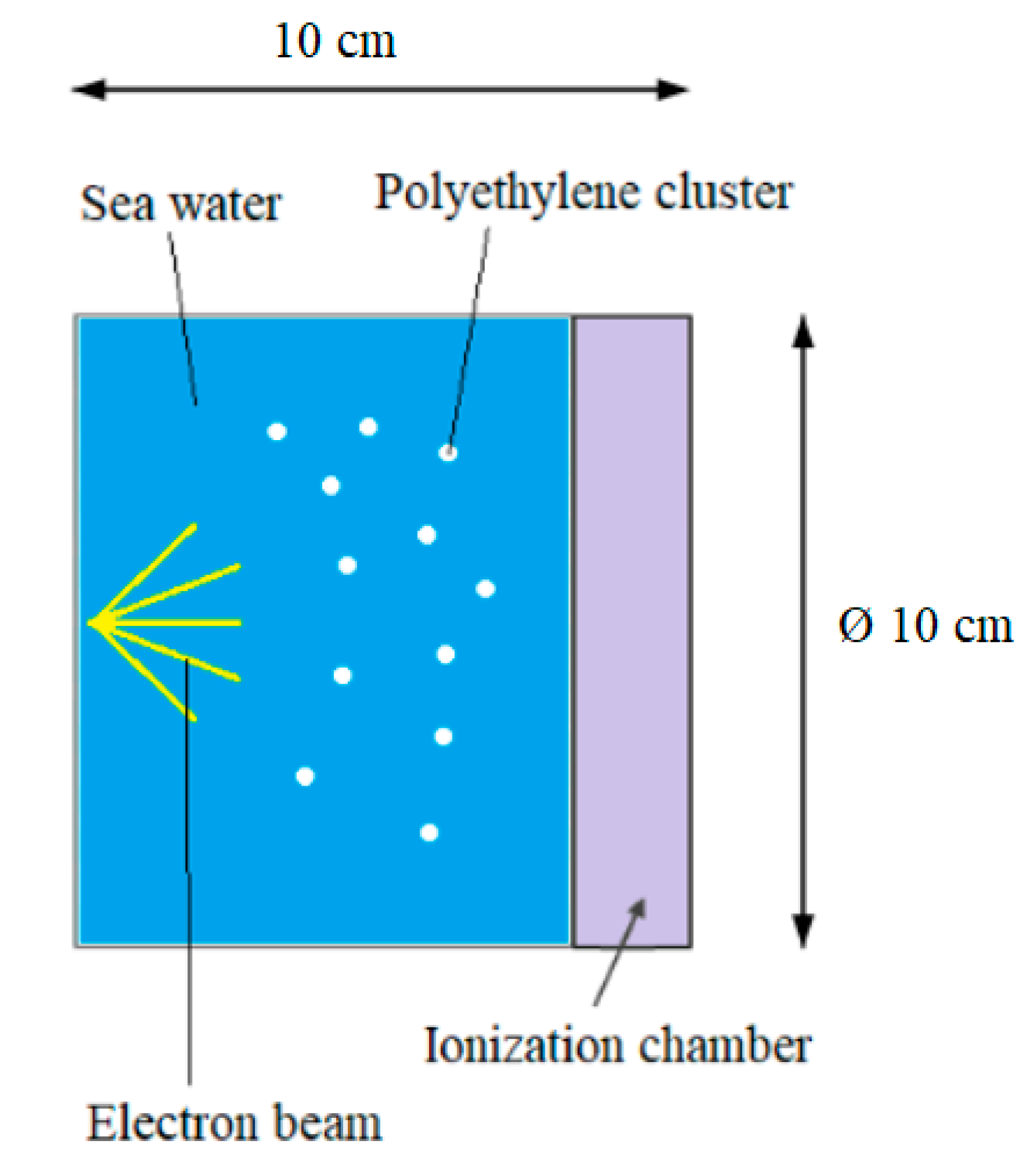
Funding

This research received no external funding.

Acknowledgments

We deeply thank: Giulio Magrin, Alessandro Alemberti, Ilaria A. Valli.

Conflicts of Interest

The authors declare no conflict of interest.

References

  1. Parker, L. Microplastics. National Geographic Society. Available online: https://www.nationalgeographic.com/environment/2019/06/microplastics-spread-throughout-deep-sea-monterey-canyon/ (accessed on 20 October 2020).
  2. Rogers, K. Microplastics “Plastic Particulate”. Britannica. Available online: https://www.britannica.com/technology/microplastic (accessed on 20 October 2020).
  3. Kane, I.A.; Clare, M.A.; Miramontes, E.; Wogelius, R.; Rothwell, J.J.; Garreau, P.; Pohl, F. Seafloor microplastic hotspots controlled by deep-sea circulation. Science 2020, 368, 1140–1145. [Google Scholar] [CrossRef] [PubMed]
  4. Smith, M.; Love, D.C.; Rochman, C.M.; Neff, R.A. Microplastics in Seafood and the Implications for Human Health. Curr. Environ. Health Rep. 2018, 5, 375–386. [Google Scholar] [CrossRef] [PubMed] [Green Version]
  5. National Research Council (US) Safe Drinking Water Committee. Drinking Water and Health; National Academies Press: Washington, DC, USA, 1977. [Google Scholar]
  6. Wesch, C.; Barthel, A.-K.; Braun, U.; Klein, R.; Paulus, M. No microplastics in benthic eelpout (Zoarces viviparus): An urgent need for spectroscopic analyses in microplastic detection. Environ. Res. 2016, 148, 36–38. [Google Scholar] [CrossRef] [PubMed]
  7. Prata, J.C.; Da Costa, J.P.; Duarte, A.C.; Rocha-Santos, T. Methods for sampling and detection of microplastics in water and sediment: A critical review. TrAC Trends Anal. Chem. 2019, 110, 150–159. [Google Scholar] [CrossRef]
  8. Maes, T.; Jessop, R.; Wellner, N.; Haupt, K.; Mayes, A.G. A rapid-screening approach to detect and quantify microplastics based on fluorescent tagging with Nile Red. Sci. Rep. 2017, 7, srep44501. [Google Scholar] [CrossRef] [PubMed] [Green Version]
  9. Araujo, C.F.; Nolasco, M.M.; Ribeiro, A.M.; Ribeiro-Claro, P.J. Identification of microplastics using Raman spectroscopy: Latest developments and future prospects. Water Res. 2018, 142, 426–440. [Google Scholar] [CrossRef] [PubMed]
  10. Marine & Environmental Research Institute. Guide to Microplastic Identification. 2012. Available online: https://docplayer.net/27438419-Guide-to-microplastic-identification.html (accessed on 20 October 2020).
  11. Segebade, C.; Starovoitova, V.N.; Borgwardt, T.; Wells, D. Principles, Methodologies, and Applications of Photon Activation Analysis: A Review; Springer: Berlin/Heidelberg, Germany, 2017. [Google Scholar]
  12. Joseph, A.; Cotruvo, W.H.O. Water, Sanitation and Health Protection and the Human Environment World; WHO: Geneva, Switzerland, 2006. [Google Scholar]
  13. Fries, E.; Dekiff, J.H.; Willmeyer, J.; Nuelle, M.T.; Ebert, M.; Remy, D. Identification of polymer types and additives in marine microplastic particles using pyrolysis-GC/MS and scanning electron microscopy. Environ. Sci. Process. Impacts 2013, 15, 1949–1956. [Google Scholar] [CrossRef] [Green Version]
  14. Bar-On, Y.M.; Phillips, R.; Milo, R. The biomass distribution on Earth. Proc. Natl. Acad. Sci. USA 2018, 115, 6506–6511. [Google Scholar] [CrossRef] [Green Version]
  15. Mann, N.H. The Third Age of Phage. PLoS Biol. 2005, 3, 753–755. [Google Scholar] [CrossRef] [Green Version]
  16. Wommack, K.E.; Colwell, R.R. Virioplankton: Viruses in Aquatic Ecosystems. Microbiol. Mol. Biol. Rev. 2000, 64, 69–114. [Google Scholar] [CrossRef] [Green Version]
  17. Suttle, C.A. Viruses in the sea. Nat. Cell Biol. 2005, 437, 356–361. [Google Scholar] [CrossRef]
  18. Bergh, O.; Børsheim, K.Y.; Bratbak, G.; Heldal, M. High abundance of viruses found in aquatic environments. Nat. Cell Biol. 1989, 340, 467–468. [Google Scholar] [CrossRef]
  19. Wigington, C.H.; Sonderegger, D.; Brussaard, C.P.D.; Buchan, A.; Finke, J.F.; Fuhrman, J.A.; Lennon, J.T.; Middelboe, M.; Suttle, C.A.; Stock, C.; et al. Re-examination of the relationship between marine virus and microbial cell abundances. Nat. Microbiol. 2016, 1, 15024. [Google Scholar] [CrossRef] [PubMed] [Green Version]
  20. Brum, J.R.; O Schenck, R.; Sullivan, M.B. Global morphological analysis of marine viruses shows minimal regional variation and dominance of non-tailed viruses. ISME J. 2013, 7, 1738–1751. [Google Scholar] [CrossRef] [Green Version]
  21. Krupovič, M.; Bamford, D.H. Putative prophages related to lytic tailless marine dsDNA phage PM2 are widespread in the genomes of aquatic bacteria. BMC Genom. 2007, 8, 236. [Google Scholar] [CrossRef] [Green Version]
  22. Xue, H.; Xu, Y.; Boucher, Y.F.; Polz, M.F. High Frequency of a Novel Filamentous Phage, VCYϕ, within an Environmental Vibrio cholerae Population. Appl. Environ. Microbiol. 2011, 78, 28–33. [Google Scholar] [CrossRef] [Green Version]
  23. Roux, S.; Krupovic, M.; Poulet, A.; Debroas, D.; Enault, F. Evolution and Diversity of the Microviridae Viral Family through a Collection of 81 New Complete Genomes Assembled from Virome Reads. PLoS ONE 2012, 7, e40418. [Google Scholar] [CrossRef]
  24. Lawrence, C.M.; Menon, S.; Eilers, B.J.; Bothner, B.; Khayat, R.; Douglas, T.; Young, M.J. Structural and Functional Studies of Archaeal Viruses. J. Biol. Chem. 2009, 284, 12599–12603. [Google Scholar] [CrossRef] [Green Version]
  25. Prangishvili, D.; Forterre, P.; Garrett, R.A. Viruses of the Archaea: A unifying view. Nat. Rev. Microbiol. 2006, 4, 837–848. [Google Scholar] [CrossRef]
  26. Mainardi, E.; Donahue, R.J.; Wilson, W.E.; Blakely, E.A. Comparison of microdosimetric simulations using PENELOPE and PITS for a 25 keV electron microbeam in water. Radiat. Res. 2004, 162, 326–331. [Google Scholar] [CrossRef] [Green Version]
  27. Vilhena, M.D.P.S.P.; Da Costa, M.L.; Berrêdo, J.F.; Paiva, R.S.; Almeida, P.D. Chemical composition of phytoplankton from the estuaries of Eastern Amazonia. Acta Amaz. 2014, 44, 513–526. [Google Scholar] [CrossRef] [Green Version]
  28. Romera-Castillo, C.; Pinto, M.; Langer, T.M.; Álvarez-Salgado, X.A.; Herndl, G.J. Dissolved organic carbon leaching from plastics stimulates microbial activity in the ocean. Nat. Commun. 2018, 9, 1–7. [Google Scholar] [CrossRef]
  29. Gin, K.Y.-H.; Lin, X.; Zhang, S. Dynamics and size structure of phytoplankton in the coastal waters of Singapore. J. Plankton Res. 2000, 22, 1465–1484. [Google Scholar] [CrossRef]
  30. Pelowitz, D.B. MCNPX User’s Manual, Version 2.5.0; Report LA-CP-05-0369; Los Alamos National laboratory: Los Alamos, NM, USA, 2005. [Google Scholar]
  31. White, M.C. Photo Atomic Data Library, MCPLIB04; Los Alamos National Laboratory: Los Alamos, NM, USA, 2003. [Google Scholar]
  32. Oak Ridge National Laboratory. MCNP-MCNPX Code Collection; Los Alamos national Laboratory: Los Alamos, NM, USA, 2006. [Google Scholar]
Figure 1. Physical model x-z section of ocean water and polyethylene.
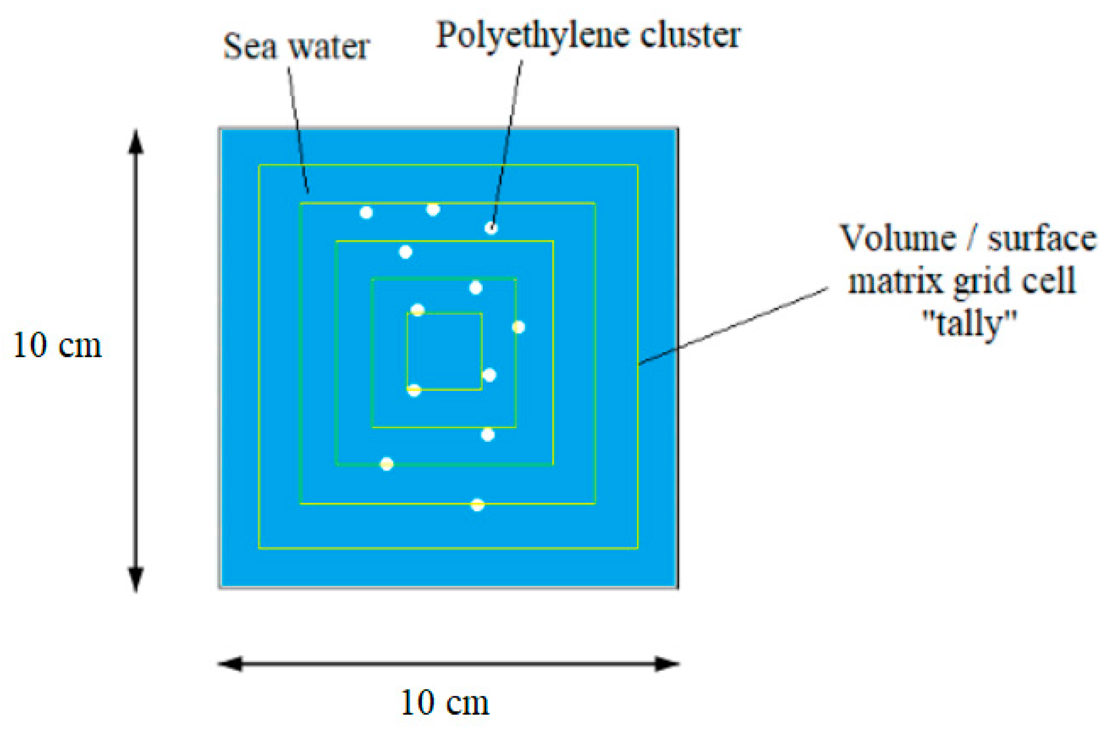
Instruments 04 00032 g001
Figure 2. Geometrical model of x-z section.
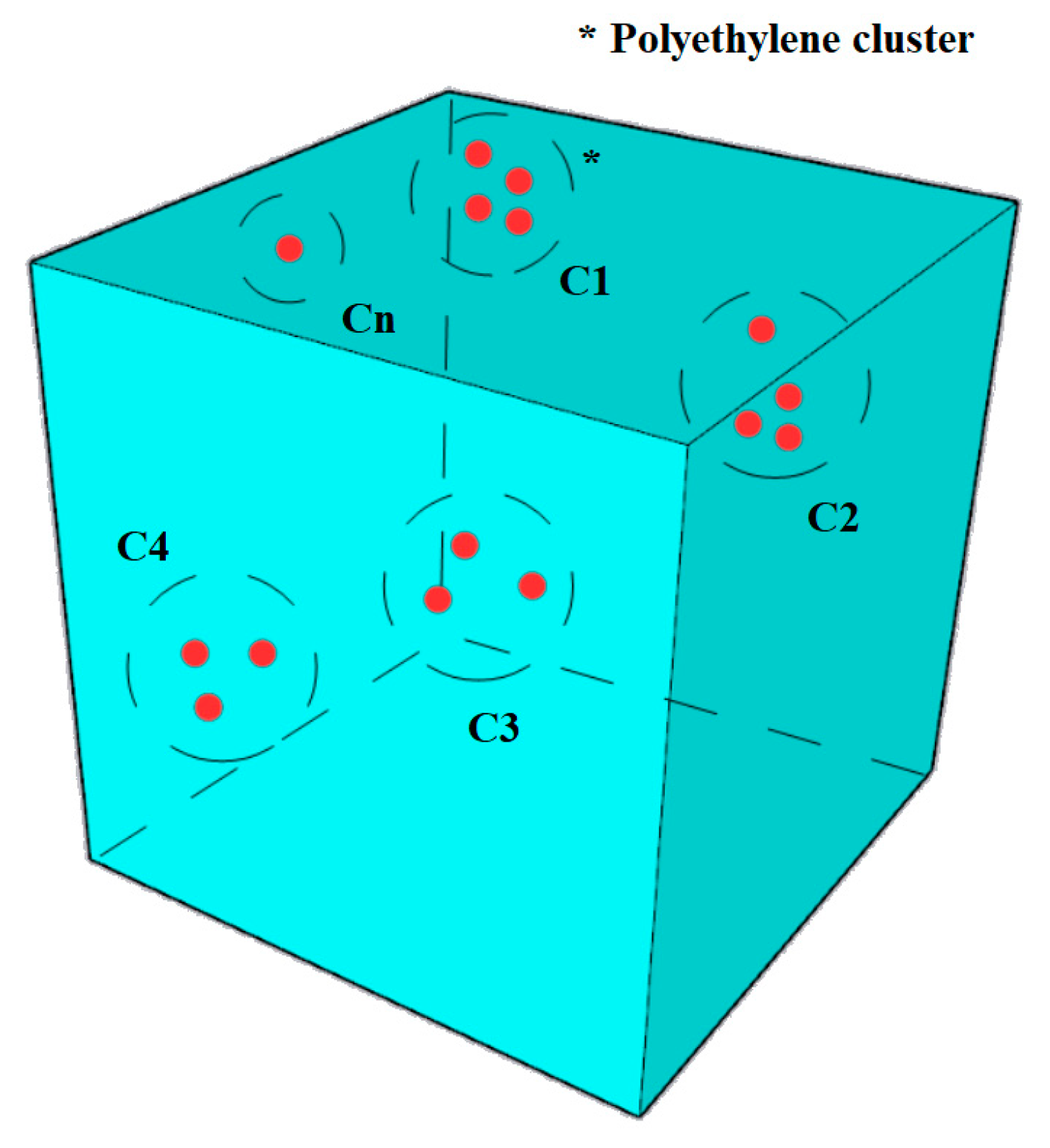
Instruments 04 00032 g002
Figure 3. Volumetric cluster cells in 3D.
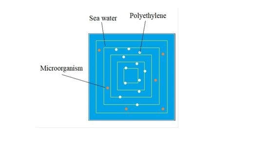
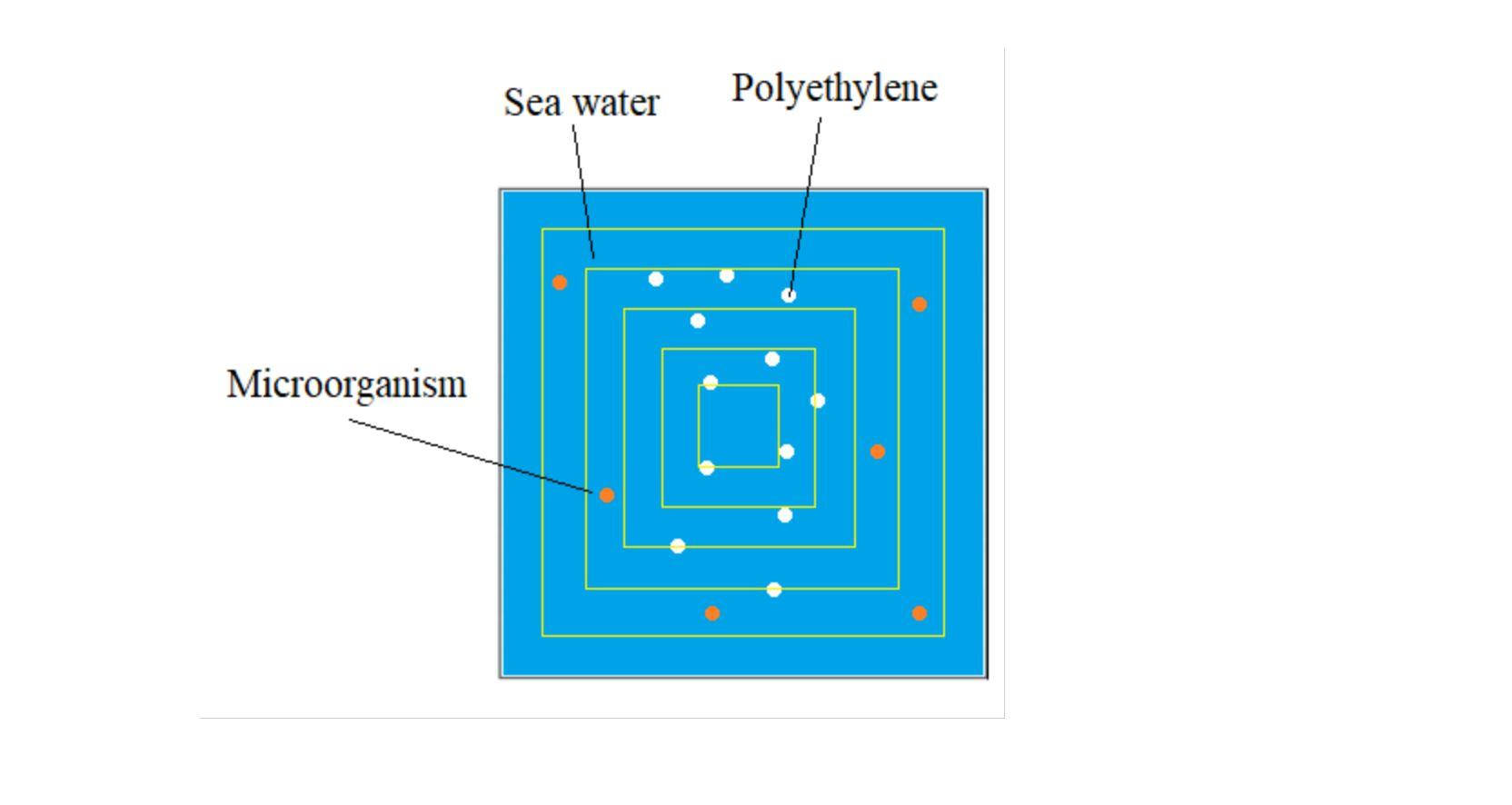
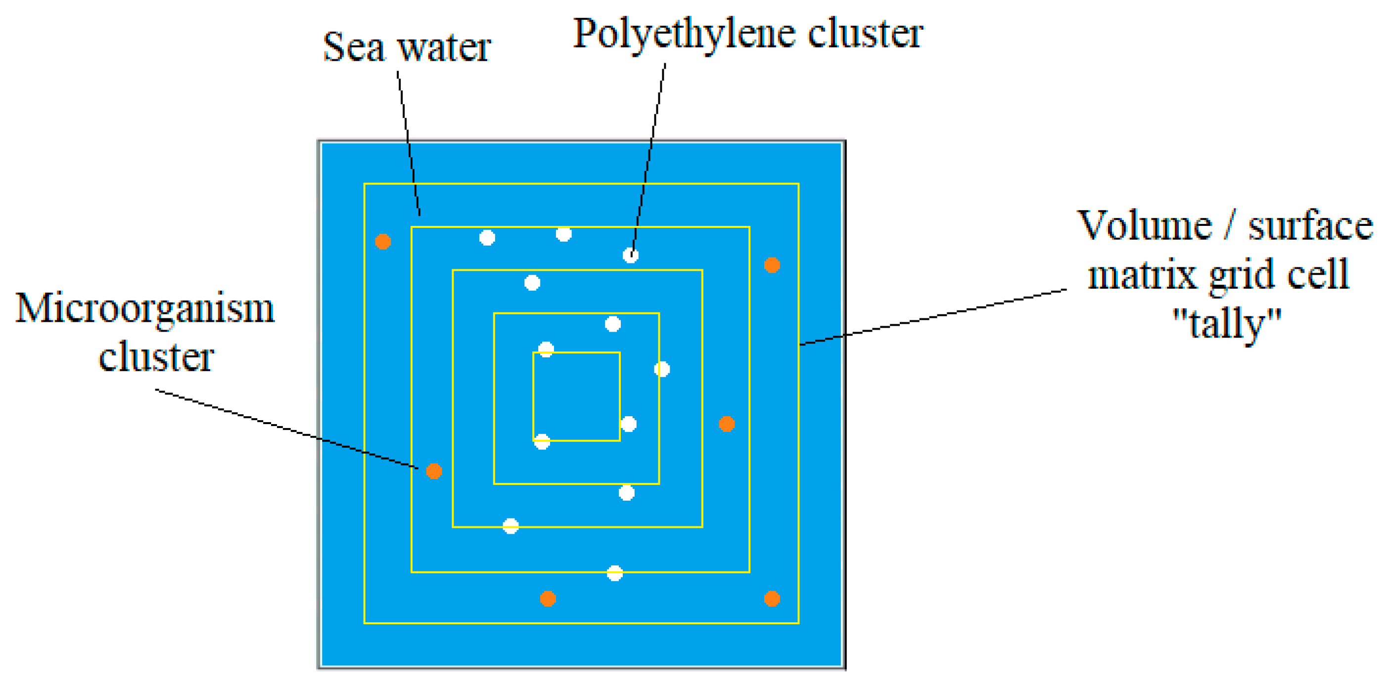
Instruments 04 00032 g003
Figure 4. Ocean water polyethylene plus microorganisms, x-z section model.
Instruments 04 00032 g004
Figure 5. Carbon total photon cross section as a function of energy.
Instruments 04 00032 g005
Figure 6. Carbon incoherent photon cross section as a function of energy.
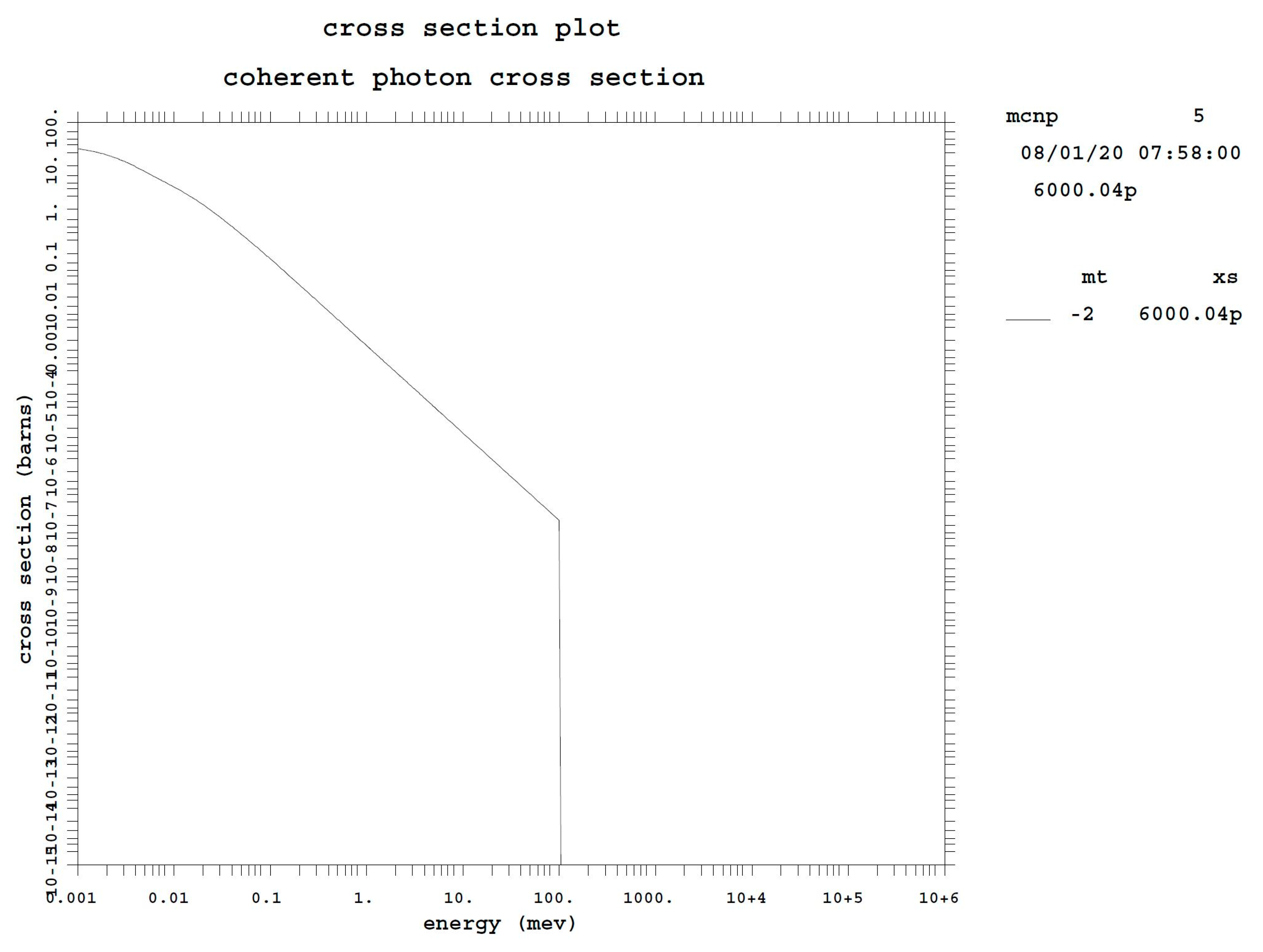
Instruments 04 00032 g006
Figure 7. Carbon coherent photon cross section as a function of energy.
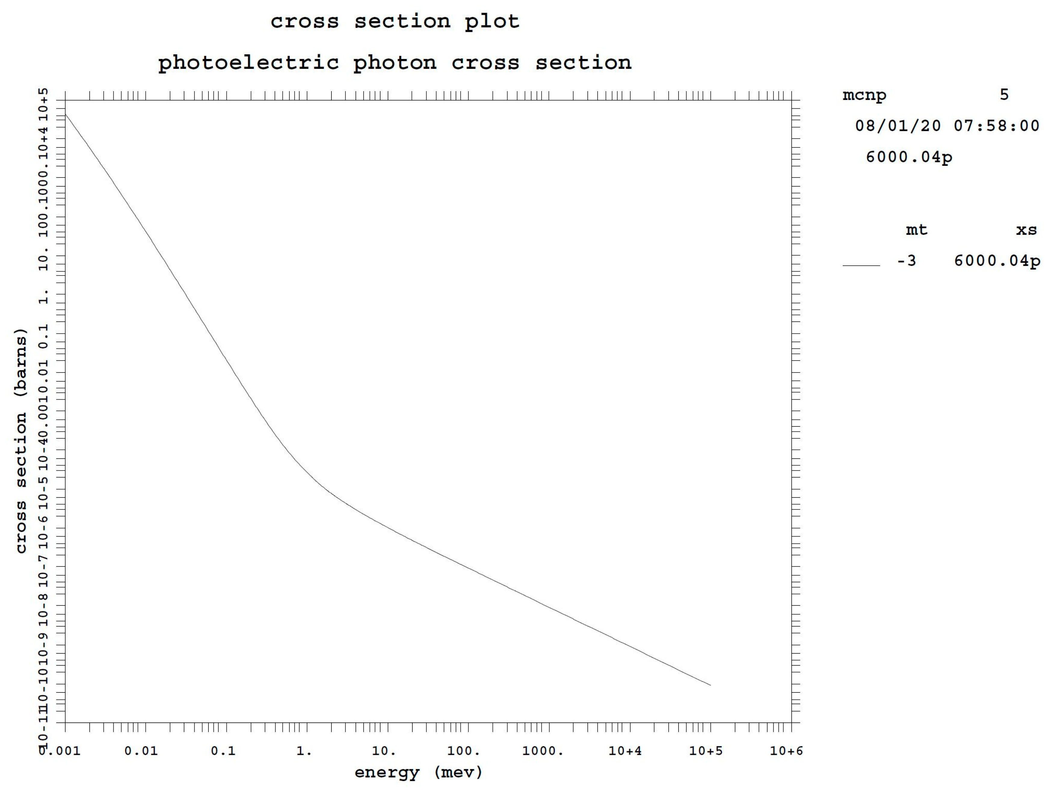
Instruments 04 00032 g007
Figure 8. Carbon photoelectric photon cross section as a function of energy.
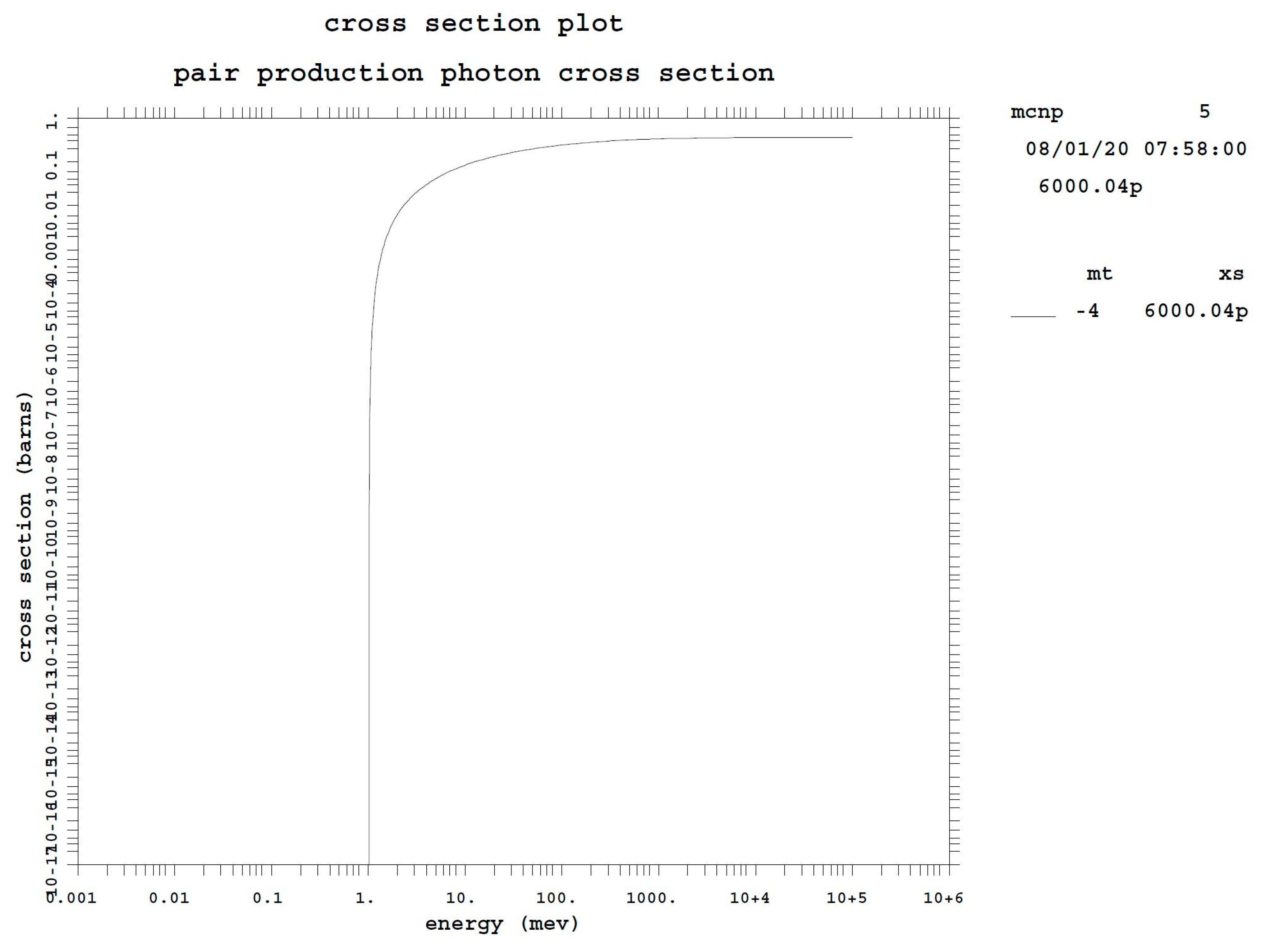
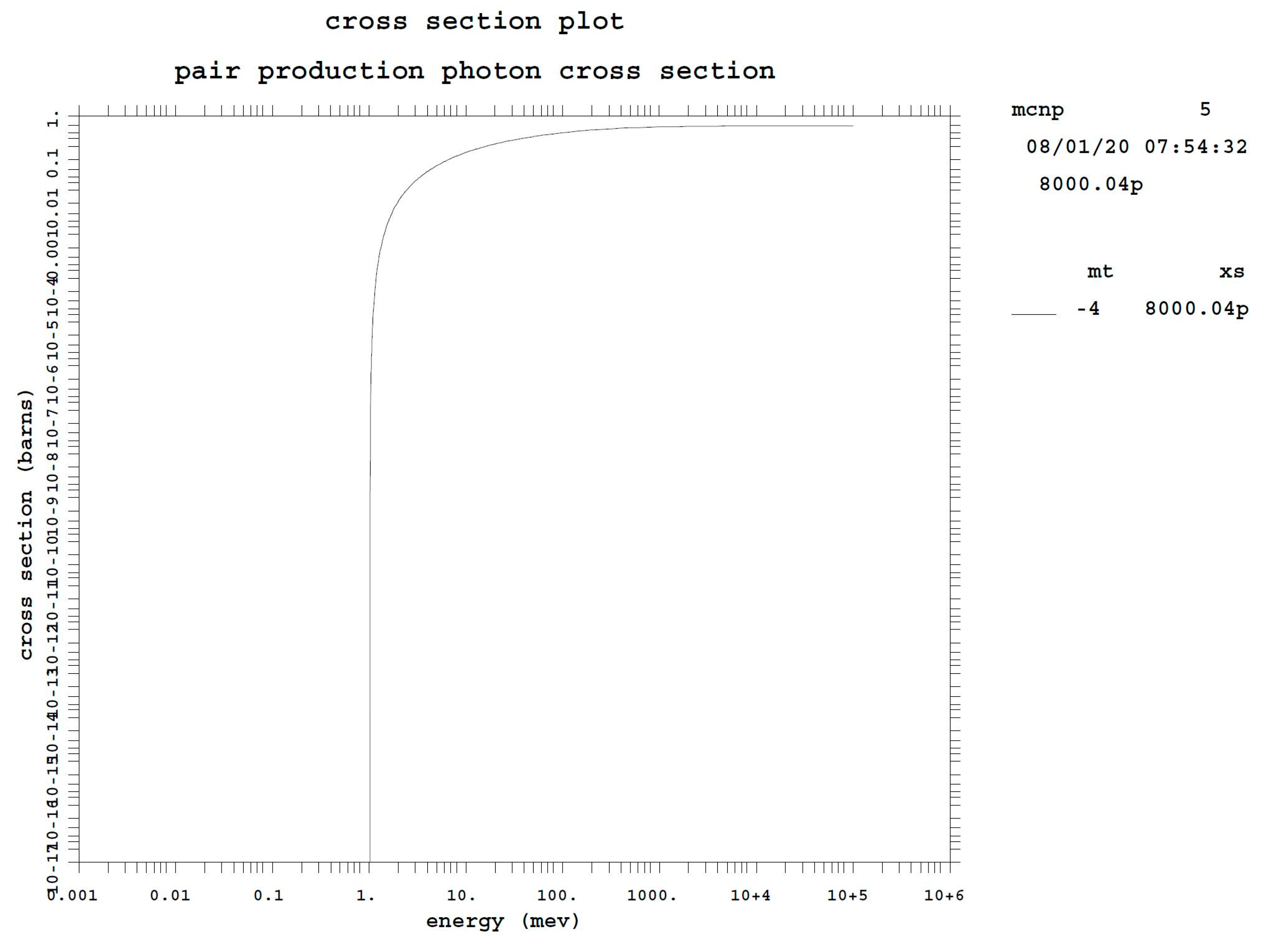
Instruments 04 00032 g008
Figure 9. Carbon pair production photon cross section as a function of energy.
Instruments 04 00032 g009
Figure 10. Oxygen total photon cross section as a function of energy.
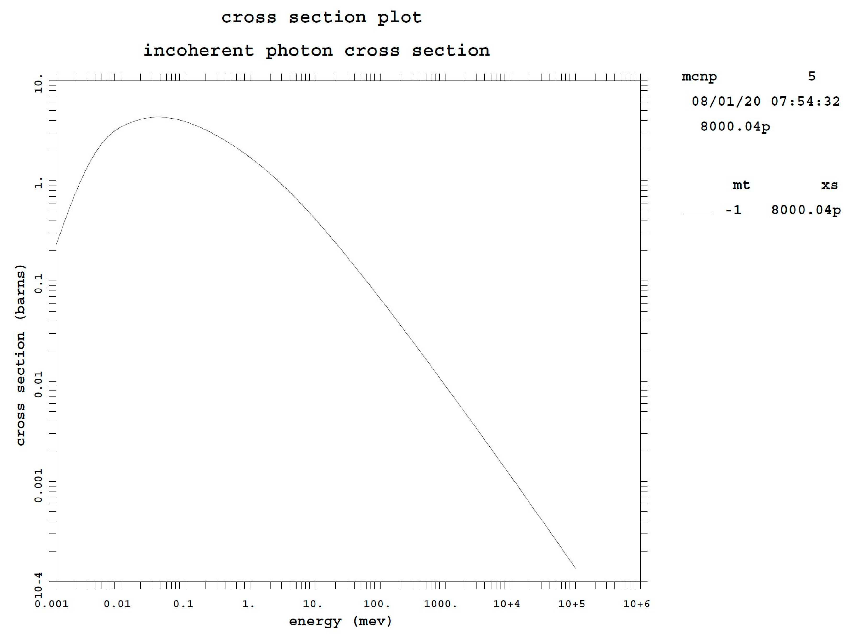
Instruments 04 00032 g010
Figure 11. Oxygen incoherent photon cross section as a function of energy.
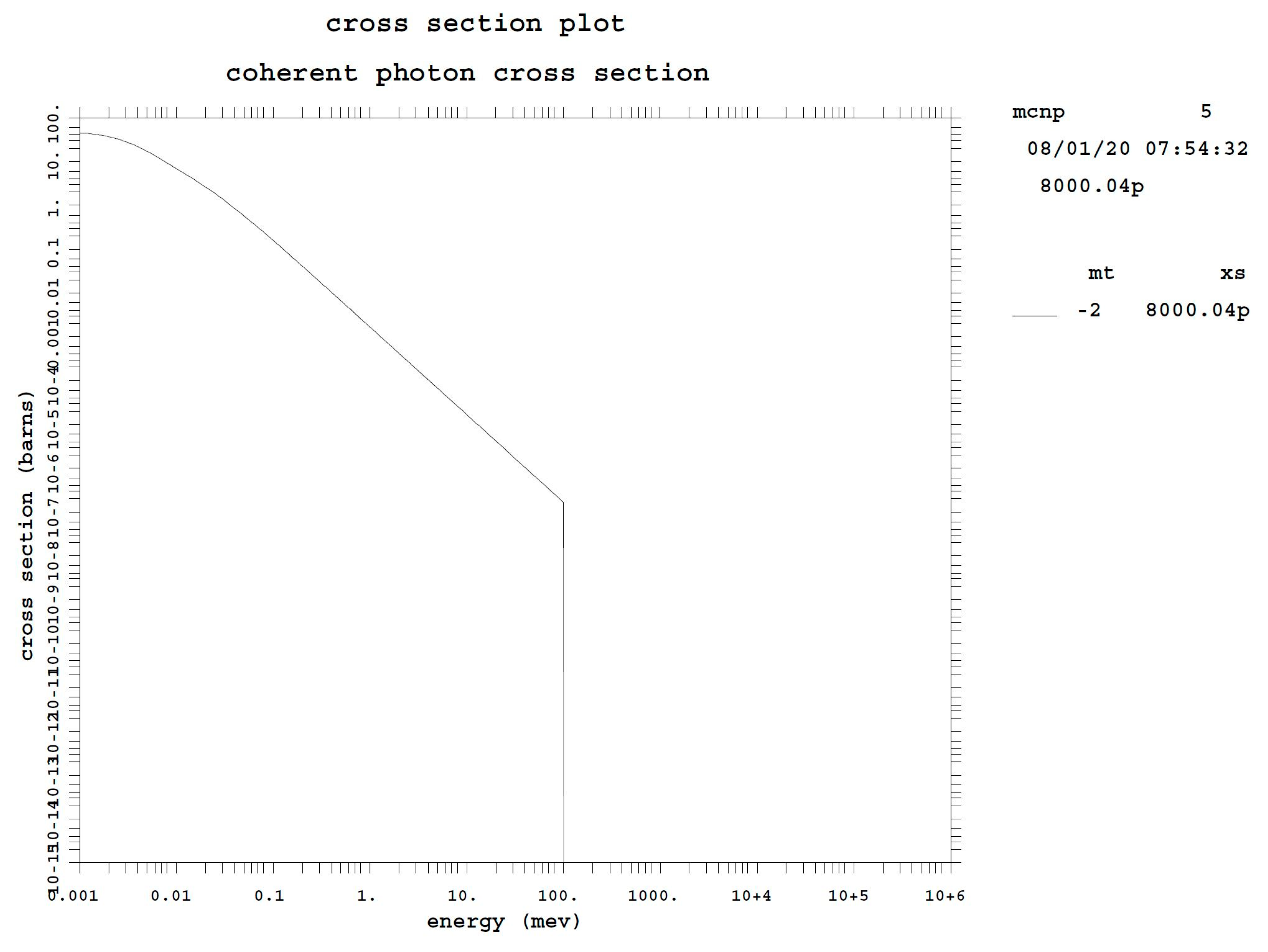
Instruments 04 00032 g011
Figure 12. Oxygen coherent photon cross section as a function of energy.
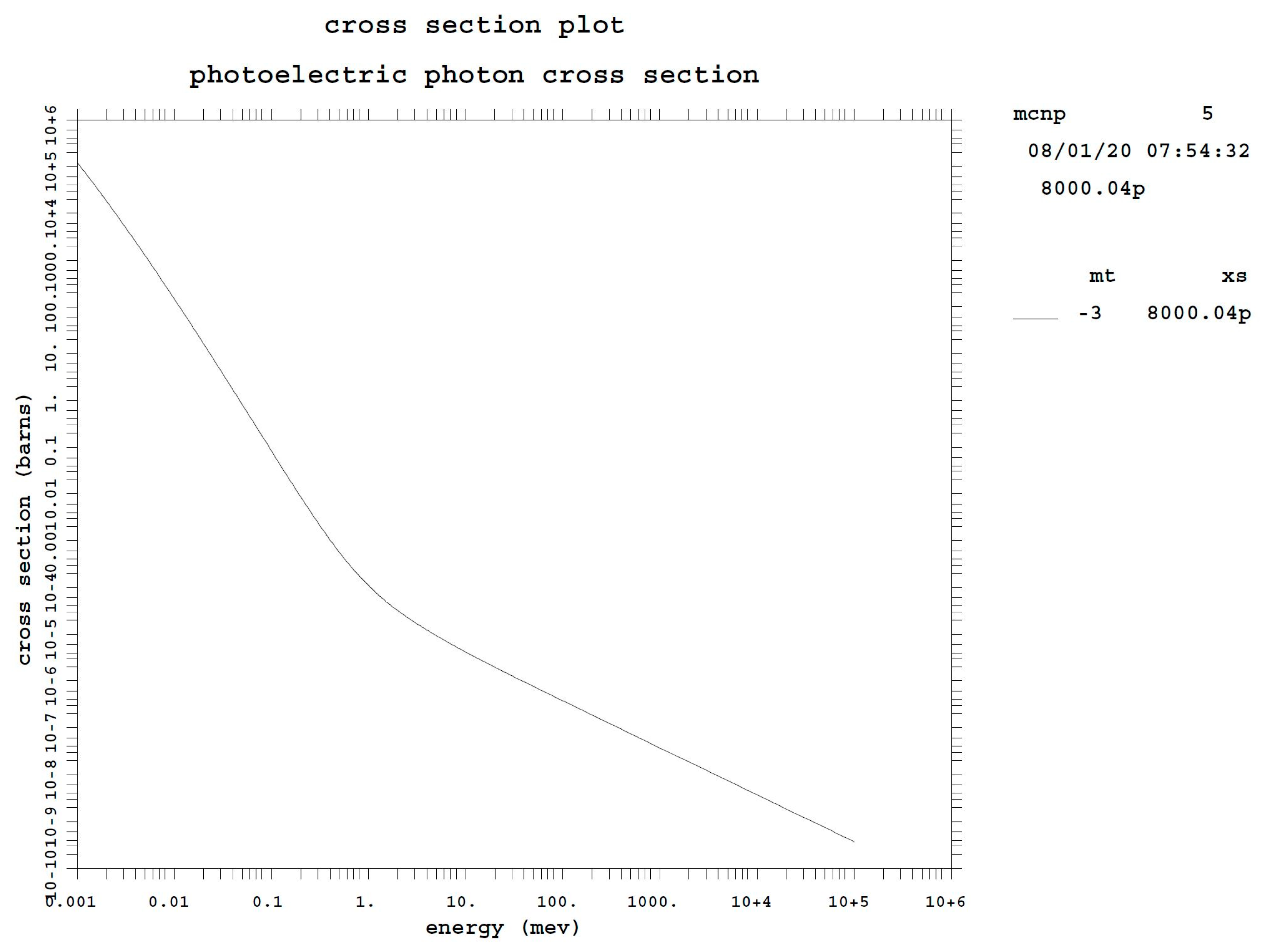
Instruments 04 00032 g012
Figure 13. Oxygen photoelectric photon cross section as a function of energy.
Instruments 04 00032 g013
Figure 14. Oxygen pair production photon cross section as a function of energy.
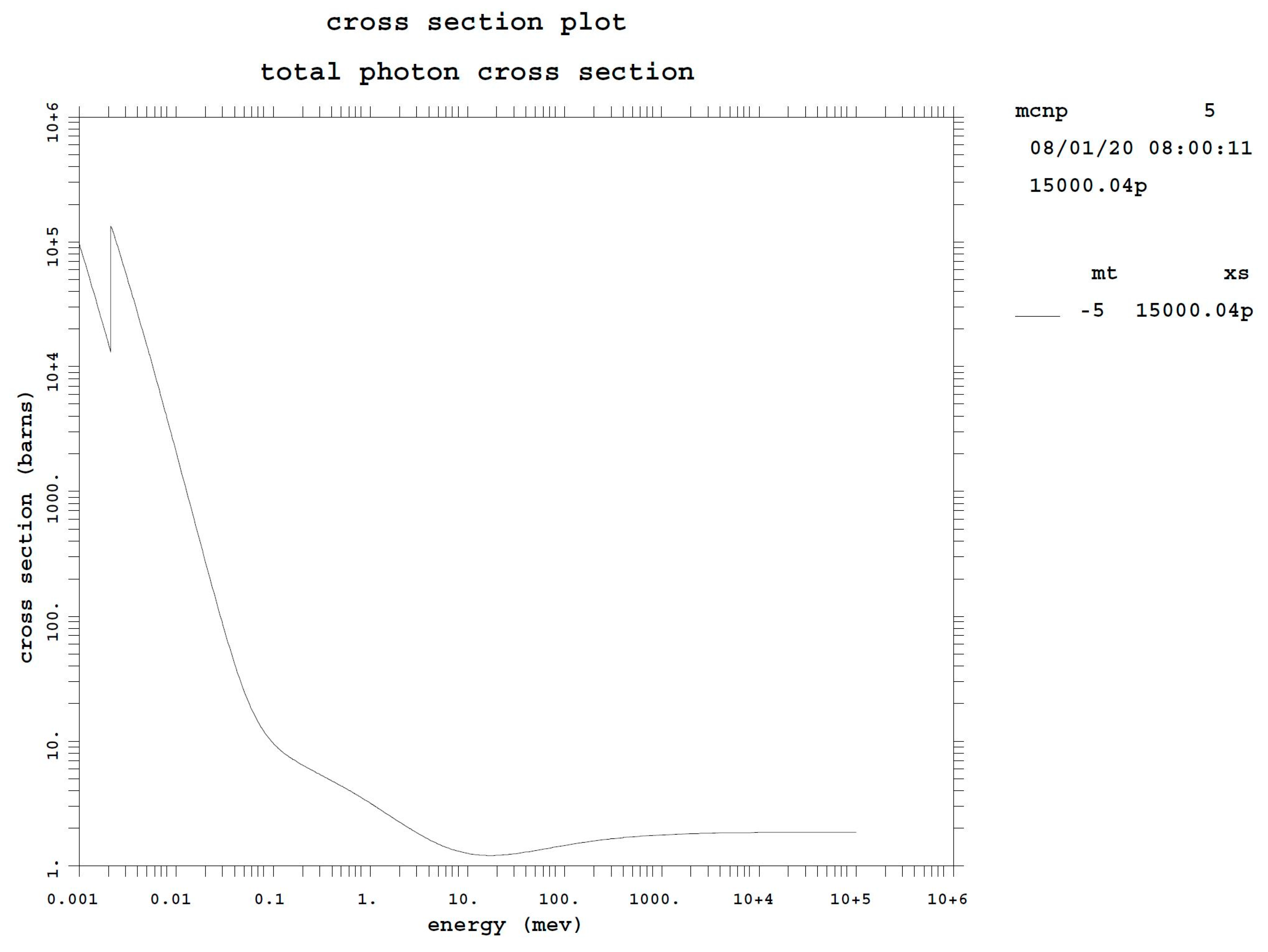
Instruments 04 00032 g014
Figure 15. Phosphorus total photon cross section as a function of energy.
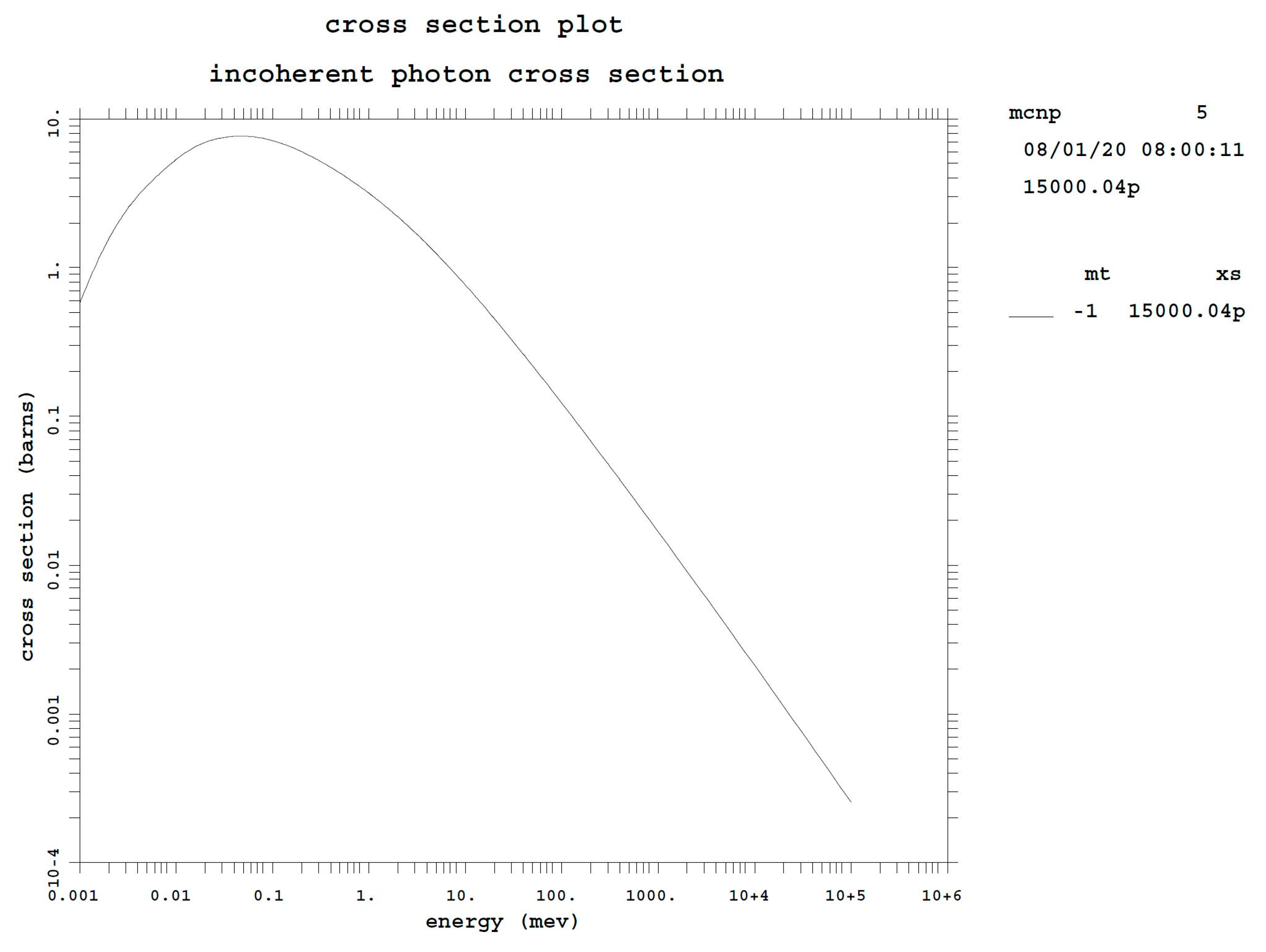
Instruments 04 00032 g015
Figure 16. Phosphorus incoherent photon cross section as a function of energy.
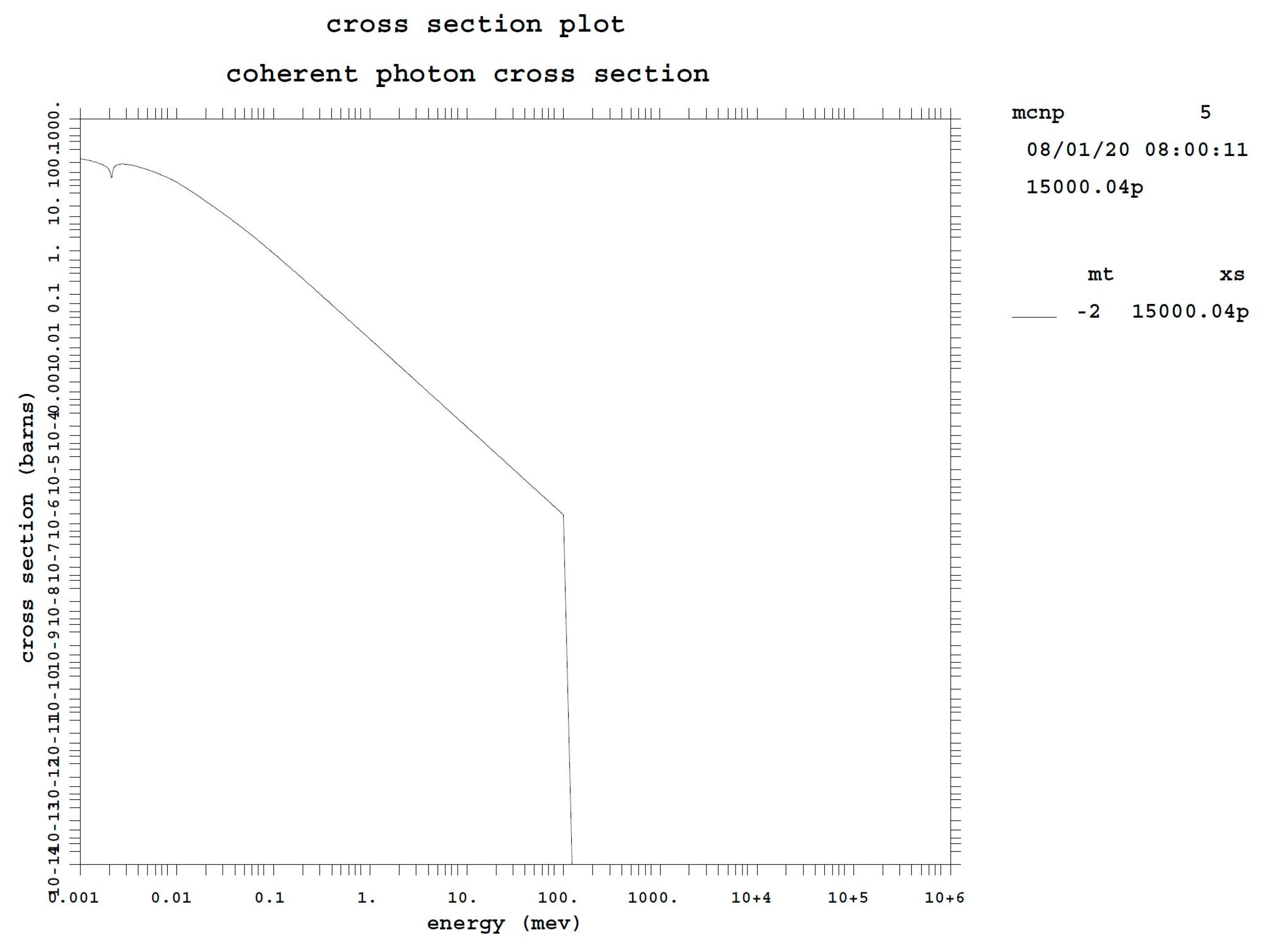
Instruments 04 00032 g016
Figure 17. Phosphorus coherent photon cross section as a function of energy.
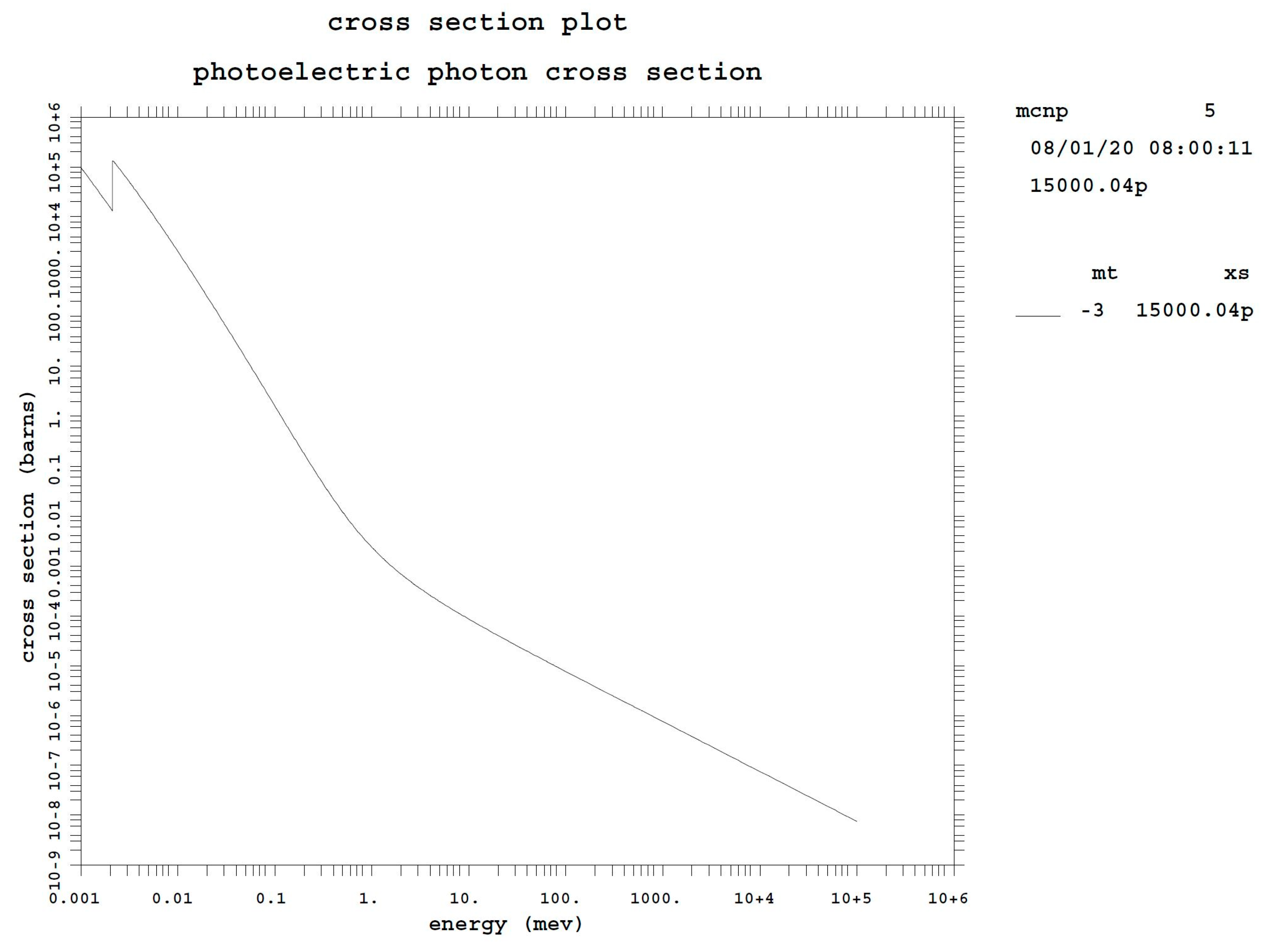
Instruments 04 00032 g017
Figure 18. Phosphorus photoelectric photon cross section as a function of energy.
Instruments 04 00032 g018
Figure 19. Phosphorus pair production photon cross section as a function of energy.
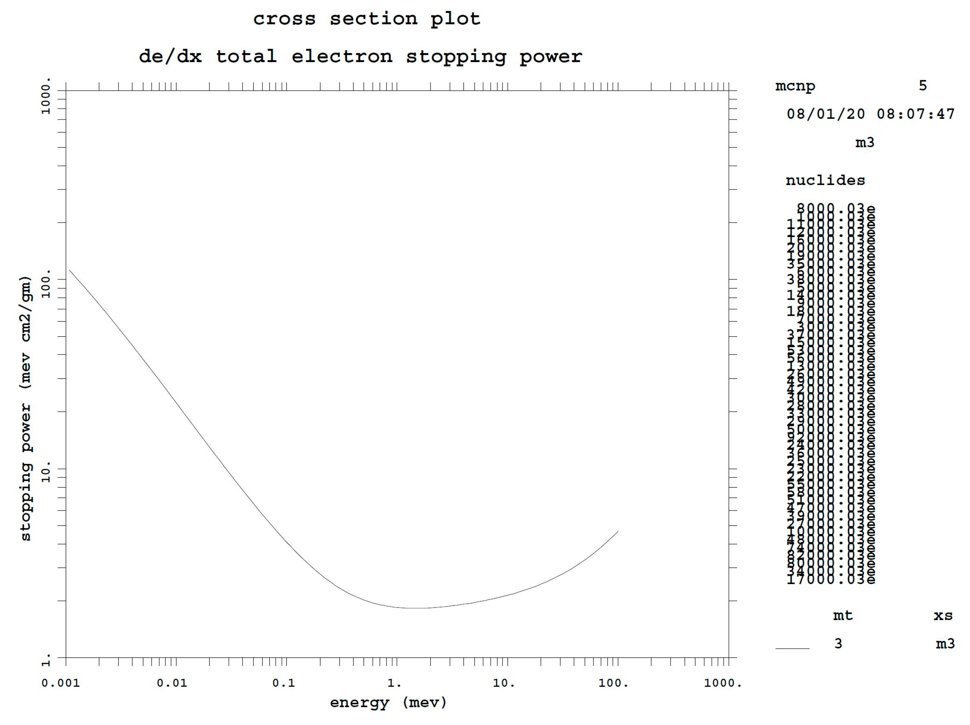
Instruments 04 00032 g019
Figure 20. Ocean water total electron stopping power as a function of energy.
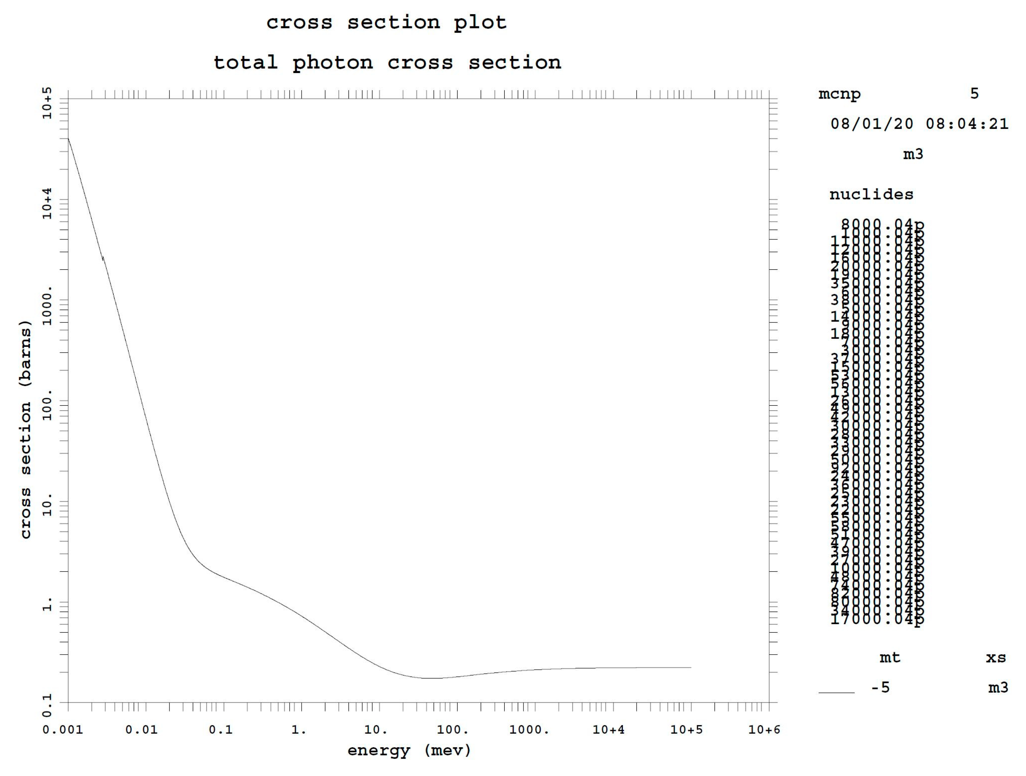
Instruments 04 00032 g020
Figure 21. Ocean water total photon cross section as a function of energy.
Instruments 04 00032 g021
Figure 22. Ocean water incoherent photon cross section as a function of energy.
Instruments 04 00032 g022
Figure 23. Ocean water coherent photon cross section as a function of energy.
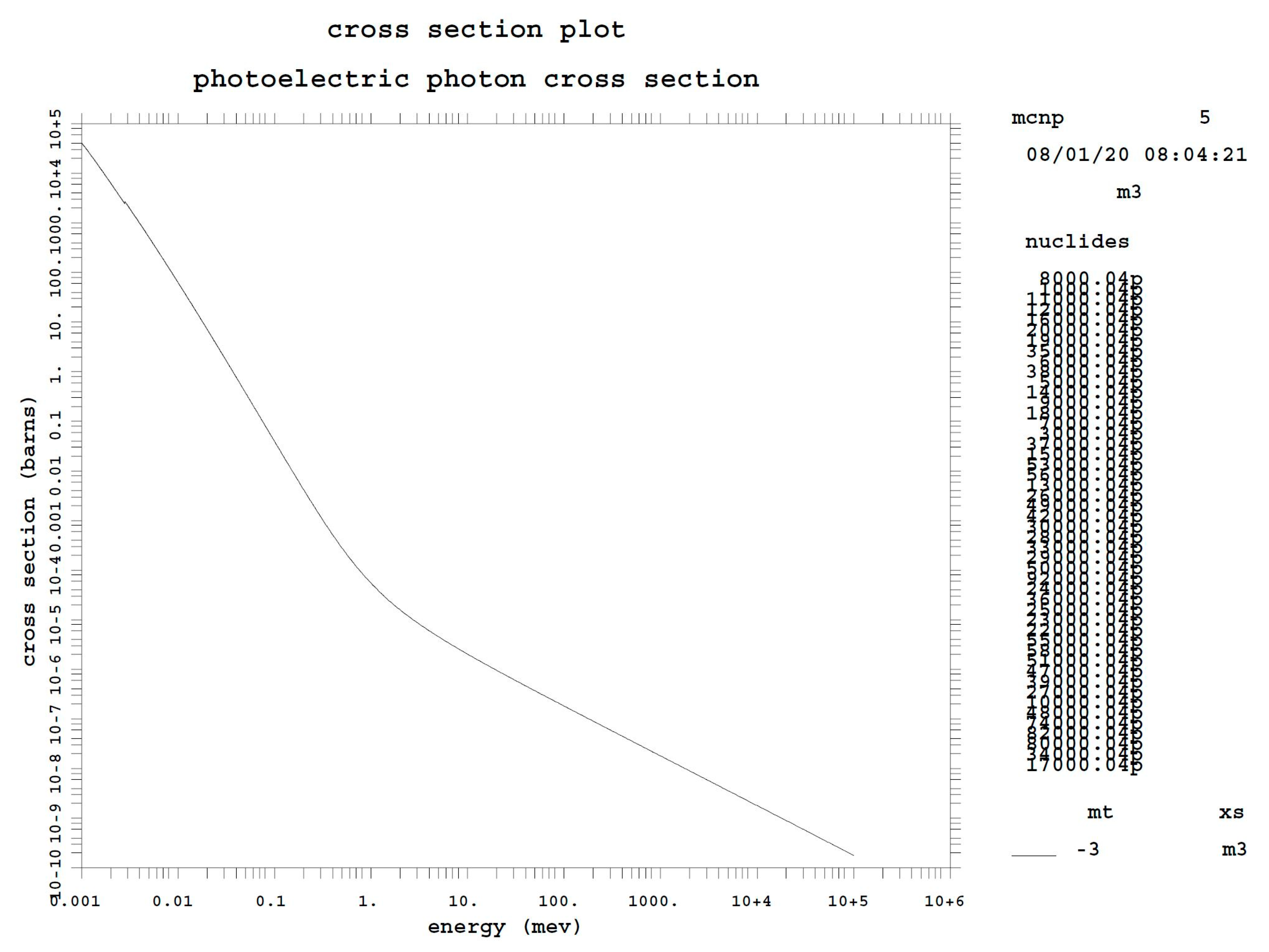
Instruments 04 00032 g023
Figure 24. Ocean water photoelectric photon cross section as a function of energy.
Instruments 04 00032 g024
Figure 25. Photon flux—ocean water vs contamination.
Instruments 04 00032 g025
Figure 26. Photon fluxes—spectrum vs contamination.
Instruments 04 00032 g026
Figure 27. 30 keV—ocean water vs contamination.
Instruments 04 00032 g027
Figure 28. 40 keV—ocean water vs contamination.
Instruments 04 00032 g028
Figure 29. 50 keV—ocean water vs contamination.
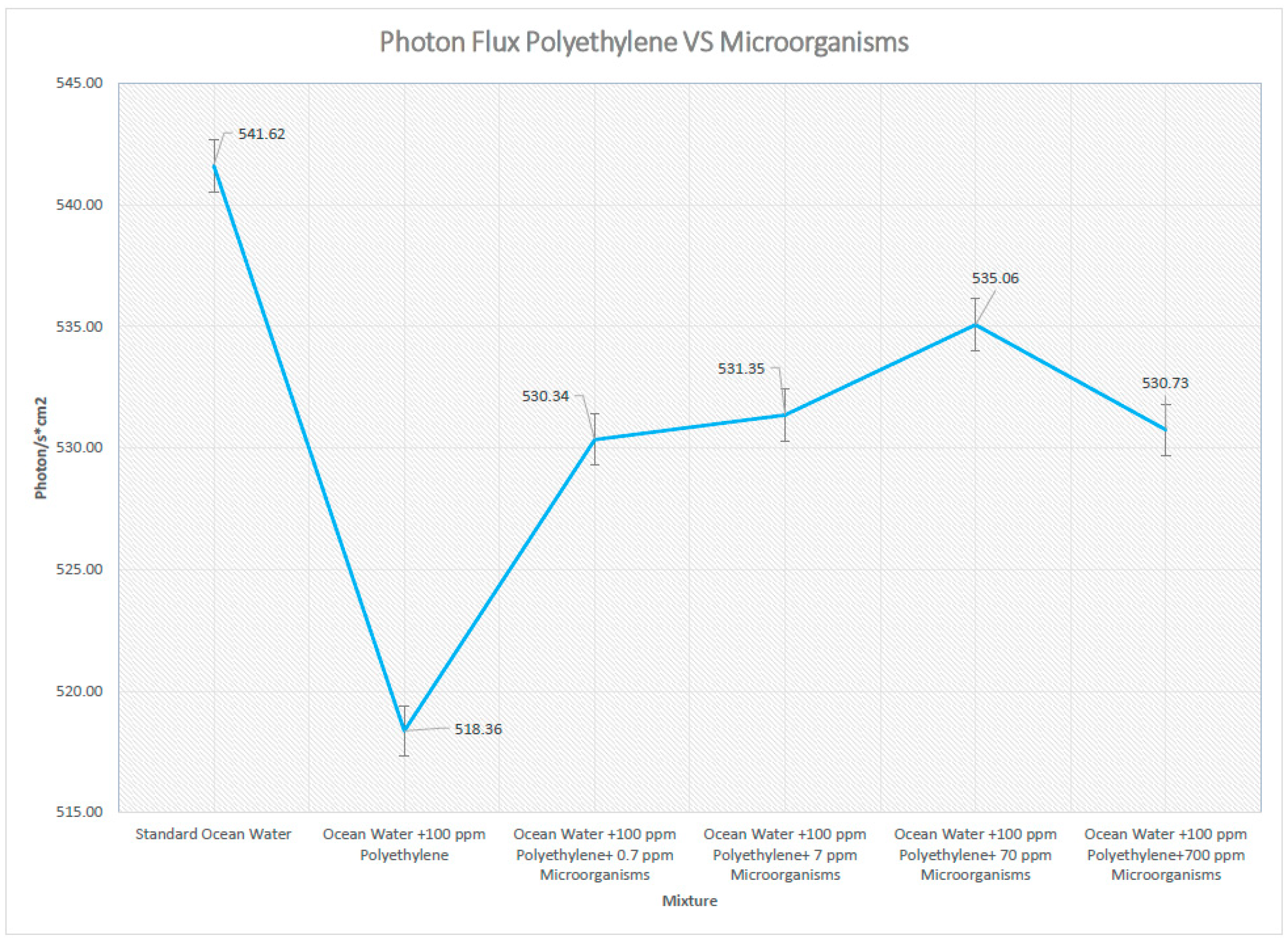
Instruments 04 00032 g029
Figure 30. Photon flux—polyethylene vs microorganisms.
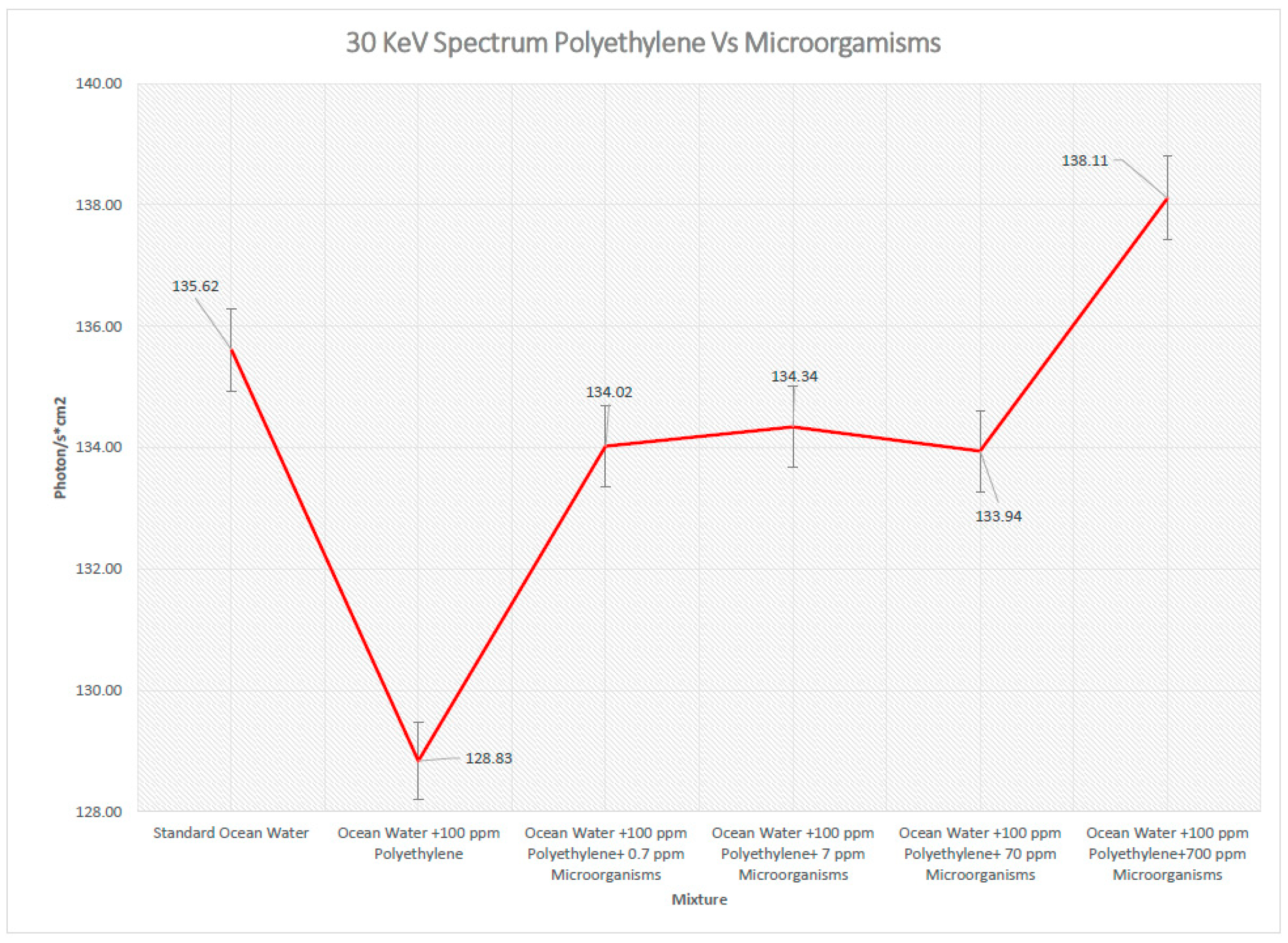
Instruments 04 00032 g030
Figure 31. 30 KeV—polyethylene vs microorganisms.
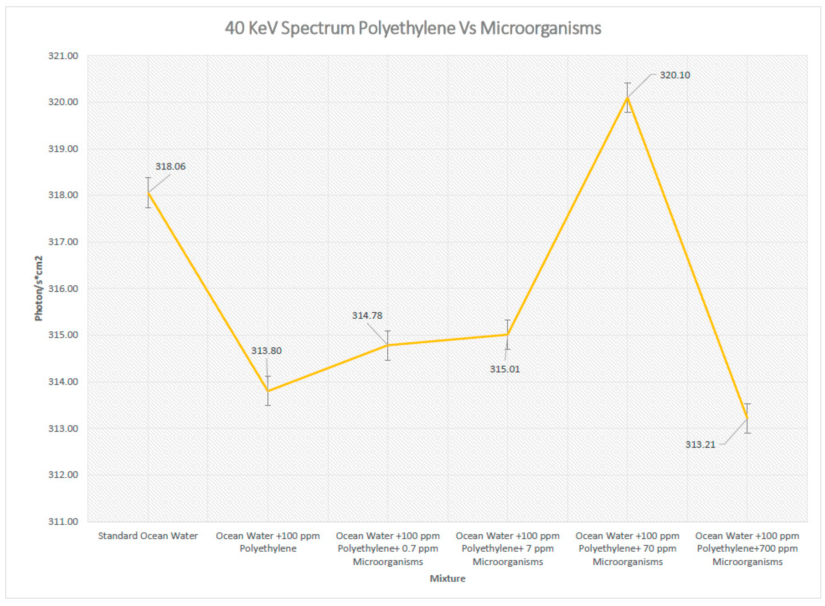
Instruments 04 00032 g031
Figure 32. 40 KeV—polyethylene vs microorganisms.
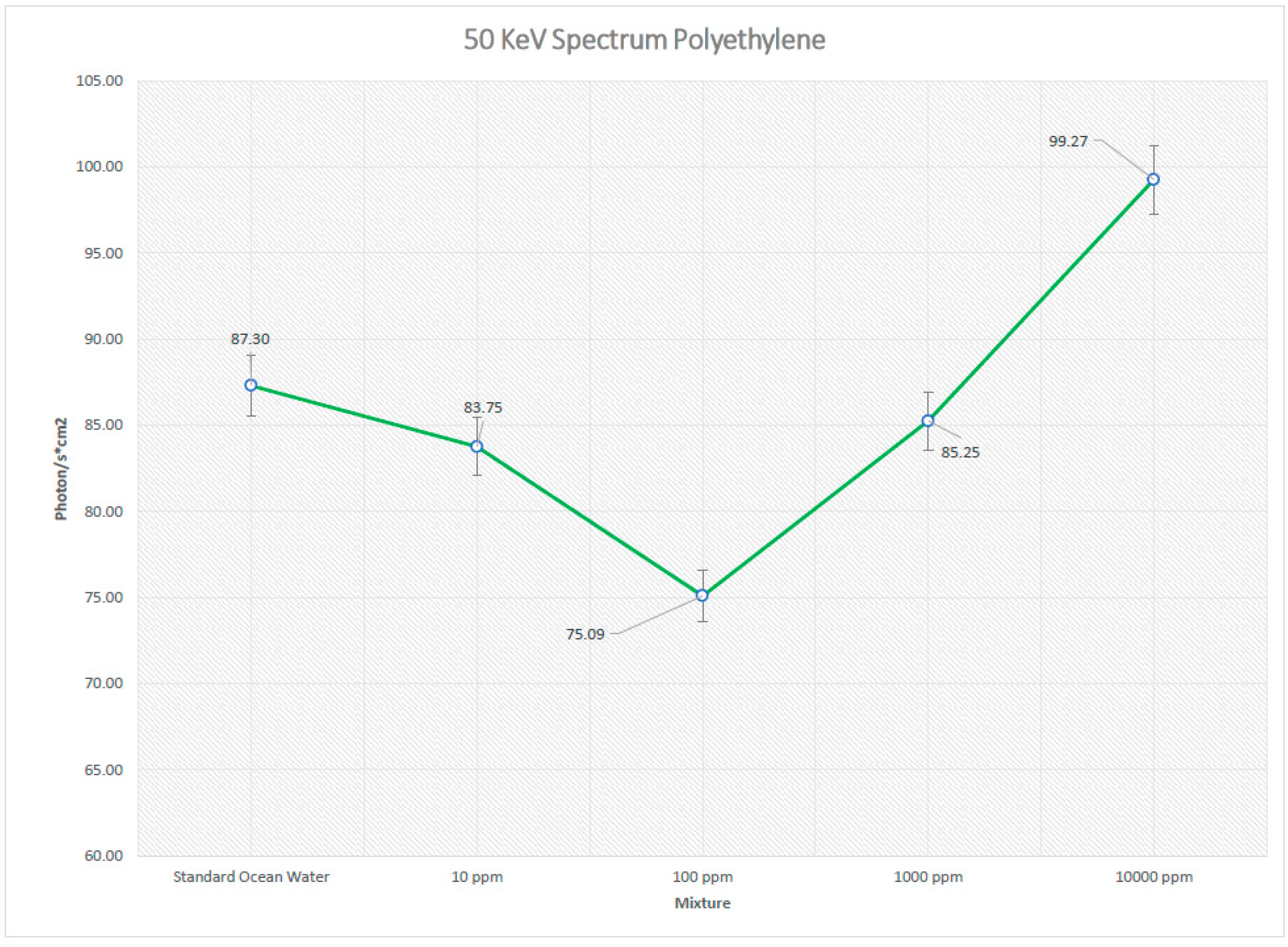
Instruments 04 00032 g032
Figure 33. 50 KeV—polyethylene vs microorganisms.
Instruments 04 00032 g033
Table 1. Ocean water weight chemical composition.
Element.Element (%)ElementElement (%)
Oxygen85.7Molybdenum0.000001
Hydrogen10.8Zinc0.000001
Chlorine1.9Nickel0.00000054
Sodium1.05Arsenic0.0000003
Magnesium0.135Copper0.0000003
Sulfur0.0885Tin0.0000003
Calcium0.04Uranium0.0000003
Potassium0.038Chromium0.00000003
Bromine0.0065Krypton0.00000025
Carbon0.0028Manganese0.0000002
Strontium0.00081Vanadium0.0000001
Boron0.00046Titanium0.0000001
Silicon0.0003Cesium0.00000005
Fluoride0.00013Cerium0.00000004
Argon0.00006Antimony0.000000033
Nitrogen0.00005Silver0.00000003
Lithium0.000018Yttrium0.00000003
Rubidium0.000012Cobalt0.000000027
Phosphorus0.000007Neon0.000000014
Iodine0.000006Cadmium0.000000011
Barium0.000003Tungsten0.00000001
Aluminum0.000001Lead0.000000005
Iron0.000001Mercury0.000000003
Indium0.000001Selenium0.000000002
Table 2. Photon Creation.
Ocean Water No ContaminationPolyethylene 10 ppmPolyethylene 100 ppmPolyethylene 1000 ppmPolyethylene 10,000 ppm
Bremsstrahlung99.1265%99.1237%99.1182%99.1545%99.3538%
1st Fluorescence0.8733%0.8755%0.8812%0.8449%0.6448%
2nd Fluorescence0.0002%0.0008%0.0006%0.0006%0.0015%
Norm100.0000%100.0000%100.0000%100.0000%100.0000%
Table 3. Nuclide Photon Activity.
ElementOcean Water No ContaminationPolyethylene 10 ppmPolyethylene 100 ppmPolyethylene 1000 ppmPolyethylene 10,000 ppm
Oxygen76.210%76.273%76.387%73.211%52.813%
Hydrogen7.585%7.405%6.998%6.686%4.259%
Chlorine12.357%12.107%12.179%11.938%8.902%
Sodium1.924%1.912%1.873%1.912%1.384%
Magnesium0.306%0.325%0.316%0.370%0.244%
Sulfur0.490%0.573%0.536%0.448%0.372%
Calcium0.429%0.512%0.434%0.409%0.277%
Potassium0.316%0.360%0.337%0.384%0.330%
Bromine0.322%0.294%0.281%0.340%0.198%
Carbon0.000%0.193%0.628%4.257%31.188%
Strontium0.056%0.046%0.031%0.044%0.029%
Silicon0.005%0.000%0.000%0.000%0.000%
Argon0.000%0.000%0.000%0.000%0.004%
Table 4. Parts per million contamination in cluster configuration.
Cluster N(10 ppm)(100 ppm)(1000 ppm)(10,000 ppm)
ppm perClusterppm perClusterppm perClusterppm perCluster
11101001000
20.5550500
32202002000
41.3131301300
51.9191901900
60.3330300
70.8880800
80.4440400
90.2220200
100.9990900
110.7770700
Norm10100100010,000
Table 5. Particles and volume in 10 ppm.
Cluster N(10 ppm)(10 ppm)Particles NVolume (mm3)
ppm per Cluster% ppm Clusterper Clusterper Cluster
1110%2621
20.55%1311
3220%5252
41.313%3411
51.919%4982
60.33%790.3
70.88%2101
80.44%1050.4
90.22%520.2
100.99%2361
110.77%1841
Norm10100.00%262311
Table 6. Particles and volume in 100 ppm.
Cluster N(100 ppm)(100 ppm)Particles NVolume (mm3)
ppm per Cluster% ppm Clusterper Clusterper Cluster
11010%262311
255%13115
32020%524522
41313%340914
51919%498321
633%7873
788%20989
844%10494
922%5252
1099%236010
1177%18368
Norm100100.00%26,227110
Table 7. Particles and volume in 1000 ppm.
Cluster N(1000 ppm)(1000 ppm)Particles NVolume (mm3)
ppm per Cluster% ppm Clusterper Clusterper Cluster
110010%26,227110
2505%13,11355
320020%52,454220
413013%34,095143
519019%49,831209
6303%786833
7808%20,98188
8404%10,49144
9202%524522
10909%23,60499
11707%18,35977
Norm1000100.00%262,2681099
Table 8. Particles and volume in 10,000 ppm.
Cluster N(10,000 ppm)(10,000 ppm)Particles NVolume (mm3)
ppm per Cluster% ppm Clusterper Clusterper Cluster
1100010%262,2681099
25005%131,134549
3200020%524,5352198
4130013%340,9481429
5190019%498,3082088
63003%78,680330
78008%209,814879
84004%104,907440
92002%52,454220
109009%236,041989
117007%183,587769
Norm10,000100.00%2,622,67610,989
Table 9. Polyethylene ppm.
CH
ppm(mg/L)(mg/L)
108.571428571.42857143
10085.714285714.2857143
1000857.142857142.857143
10,0008571.428571428.57143
Table 10. Ocean Water Vs Polyethylene ppm composition.
ElementOrigin Element (%)Element (ppm)10 ppm Polyethylene (ppm)100 ppm Polyethylene (ppm)1000 ppm Polyethylene (ppm)10,000 ppm Polyethylene (ppm)
Oxygen85.708.57 × 1058.570 × 1058.569 × 1058.561 × 1058.484 × 105
Hydrogen10.801.08 × 1051.080 × 1051.080 × 1051.081 × 1051.094 × 105
Chlorine1.9019,0001.900 × 1041.900 × 1041.898 × 1041.881 × 104
Sodium1.0510,5001.050 × 1041.050 × 1041.049 × 1041.040 × 104
Magnesium0.1413501.350 × 1031.350 × 1031.349 × 1031.337 × 103
Sulfur0.098858.850 × 1028.849 × 1028.841 × 1028.762 × 102
Calcium0.044004.000 × 1024.000 × 1023.996 × 1023.960 × 102
Potassium0.043803.800 × 1023.800 × 1023.796 × 1023.762 × 102
Bromine0.01656.500 × 1016.499 × 1016.494 × 1016.435 × 101
Carbon0.00283.657 × 1011.137 × 1028.851 × 1028.599 × 103
Publisher’s Note: MDPI stays neutral with regard to jurisdictional claims in published maps and institutional affiliations.

