Real-Time LFO Damping Enhancement in Electric Networks Employing PSO Optimized ANFIS

Abstract

In recent years, machine learning (ML) tools have gained tremendous momentum and received wide-spread attention in different segments of modern-day life. As part of digital transformation, the power system industry is one of the pioneers in adopting such attractive and efficient tools for various applications. Apparently, a nonthreatening, but slow-burning issue of the electric power systems is the low-frequency oscillations (LFO), which, if not dealt with appropriately and on time, could result in complete network failure. This paper addresses the role of a prominent ML family member, particle swarm optimization (PSO) tuned adaptive neuro-fuzzy inference system (ANFIS) for real-time enhancement of LFO damping in electric power system networks. It adopts and models two power system networks where in the first network, the synchronous machine is equipped with only a power system stabilizer (PSS), and in the other, the PSS of the synchronous machine is coordinated with the unified power flow controller (UPFC), a second-generation flexible alternating current transmission system (FACTS) device. Then, it develops the proposed ML approach to enhance LFO damping for both adopted networks based on the customary practices of statistical judgment. The performance measuring metrics of power system stability, including the minimum damping ratio (MDR), eigenvalue, and time-domain simulation, were used to analyze the developed approach. Moreover, the paper presents a comparative analysis and discussion with the referenced works’ achieved results to conclude the proposed PSO-ANFIS technique’s ability to enhance power system stability in real-time by damping out the unwanted LFO.

1. Introduction

Energy demand is increasing gradually due to the growing population. To meet this increased energy demand, modern power systems are typically operated at their highest capacity. Under this situation, the power systems utilize their maximum ability, and therefore, the operation is economical. However, this situation leads the system to violate the system constraints. As a result, the system parameters become oscillatory, which eventually leads to system instability. In addition, recently, the trend in power systems has been to integrate renewable energy sources at the maximum possible capacity, which helps to decrease the dependency on fossil fuels and make the overall system environmentally friendly. However, the intermittent nature of these renewable energy sources causes low-frequency oscillations (LFO) in power networks. The frequency range of 0.1–2.5 Hz is the main dominating frequency for LFO [1], and it severely affects those power networks that are interconnected through weak tie lines. Poor damping of LFO causes dynamic instability and leads to the whole grid’s blackouts in some cases [2].

To protect the power networks from such a scenario, necessary damping must be provided at the right time to manage the LFO. Although a healthy number of research works were conducted during the last few decades, there is further scope for contributions in this area. An automatic voltage regulator (AVR) is one possible solution proposed by the researchers, where the generator excitation is controlled to manage the LFO issue. However, the synchronous generators with high-gain AVR decrease the damping torque of rotors, which increases the LFO [3]. In such cases, system stability can be enhanced by mitigating the LFO problem using a power system stabilizer with an AVR-based excitation control technique [4]. Appropriate adjustment of the PSS parameters is the critical factor in terms of achieving a highly effective approach. Different approaches to this challenging task are addressed in [5].

On the other hand, the development of the power electronics technology introduced wide-spread use of the flexible alternating current transmission system (FACTS) devices in electric power networks. In references [6,7,8], the authors analyzed the power system networks’ steady-state performance by incorporating the FACTS devices and shown significant improvement. The dynamic parameters of the power networks, including voltage, current, phase angle, and impedance, were also improved with the aid of FACTS devices [9]. Typically, FACTS devices are employed in power systems to improve overall system performance. The improvement of the power network stability by mitigating inter-area LFO, maintaining a satisfactory voltage profile, supplying optimal power, and dispatching reactive power to the network was reported successively [10,11,12,13]. Incorporating the FACTS devices into the system, the analysis of these power system parameters was conducted through artificial intelligence algorithms. The available three common structures of these devices are shunt, series, and a combination of them. One of the most comprehensive multifunctional FACTS devices is the unified power flow controller (UPFC), which comprises both the functional effects of series and shunt systems [14]. The power system network parameters, such as line reactance, bus voltage, and phase angle of the bus voltages, can be adjusted with the deployment of UPFC. They can increase the controlling profile of the steady-state power flow among the transmission lines. It can also improve the transient stability, voltage regulation, LFO profile, and minimization of power loss [15,16,17]. The stability of the single machine infinite bus (SMIB) network was investigated through a static series synchronous compensator, where the parameters were optimized by particle swarm optimization (PSO) [18] and teacher learner-based optimization (TLBO) [19]. The continuous coordination of PSS and a thyristor controlled series capacitor was designed using the dolphin echolocation optimization (DEO) technique for the SMIB network stability improvement, as reported in [20]. The damping out of LFO employing UPFC mainly depends on the tuning strategy of its control parameters. Proper coordination between power system stabilizer (PSS) and UPFC must be ensured to achieve system stability through the necessary suppression of the LFO [21]. Therefore, several artificial intelligence techniques were implemented previously to optimize the PSS parameters coordinated with/without FACTS devices, which include the water cycle algorithm (WCA) [21], genetic algorithm (GA) [22], backtracking search algorithm (BSA) [23,24], particle swarm optimization (PSO) [25], and differential evolution (DE) [26]. However, most of these methods are implemented in offline mode operations and can tune the PSS parameters for a particular operating condition. As a result, the mentioned parameter-setting techniques for PSS are not suitable for the real-time operation of power systems as the operating points of power networks are constantly changing. On the other hand, online/real-time parameter tuning of PSS was conducted using some artificial intelligence techniques, which include support vector machine (SVM) [27], artificial neural network (ANN) [28], genetic programming (GP) [29], and extreme learning machine (ELM) [30]. Hybridization of ANN with other algorithms was also applied successfully in many other power system applications [31] besides PSS parameter tuning. A neuro-fuzzy algorithm based nonlinear model-free robust controller was proposed for damping out the LFO from any power system to replace the conventional PSS in [32]. An intelligent control approach, namely the neuro-fuzzy intelligent controlling technique, was applied to control newly developed real-time dynamics [33]. However, real-time based parameter settings can be achieved by employing another highly efficient machine learning approach, PSO tuned adaptive neuro-fuzzy inference system (ANFIS) to improve the overall system stability. PSO tuned ANFIS models were implemented in various scenarios, such as viscosity estimation of an oil mixture [34] and predicting the wave reflection coefficient for semicircular breakwater considering a range of wave heights [35]. Therefore, in this paper, a PSO-tuned ANFIS approach was implemented to achieve real-time tuning of the PSS parameters. The stability indicators of the power system were analyzed to determine the performance. The technique was implemented in two different electric networks to show the effectiveness of the approach. One electric power network is made of a SMIB system with PSS only, and the other one is a SMIB system with UPFC coordinated PSS. The efficiency of the PSO-ANFIS machine learning tool was investigated through minimum damping ratio (MDR) and eigenvalue analyses. The proposed technique’s superiority was established by comparing it with the conventional and the literature reported approaches for several loading conditions. Some other statistical performance indices (SPI) including the root mean squared error (RMSE), mean absolute percentage error (MAPE), RMSE-observations to standard deviation ratio (RSR), coefficient of determination (R²), and Willmott’s index of agreement (WIA) were also evaluated to explore the robustness of the proposed machine learning model. The superiority of the proposed method over the conventional one was determined by comparing time-domain simulation results. The main contributions of this research are as follows:

• Two versions of SMIB electric networks were considered to demonstrate the proposed approach of LFO mitigation. For both the networks, optimized PSS parameters were found offline for a large number of operating conditions using a heuristic optimization technique.
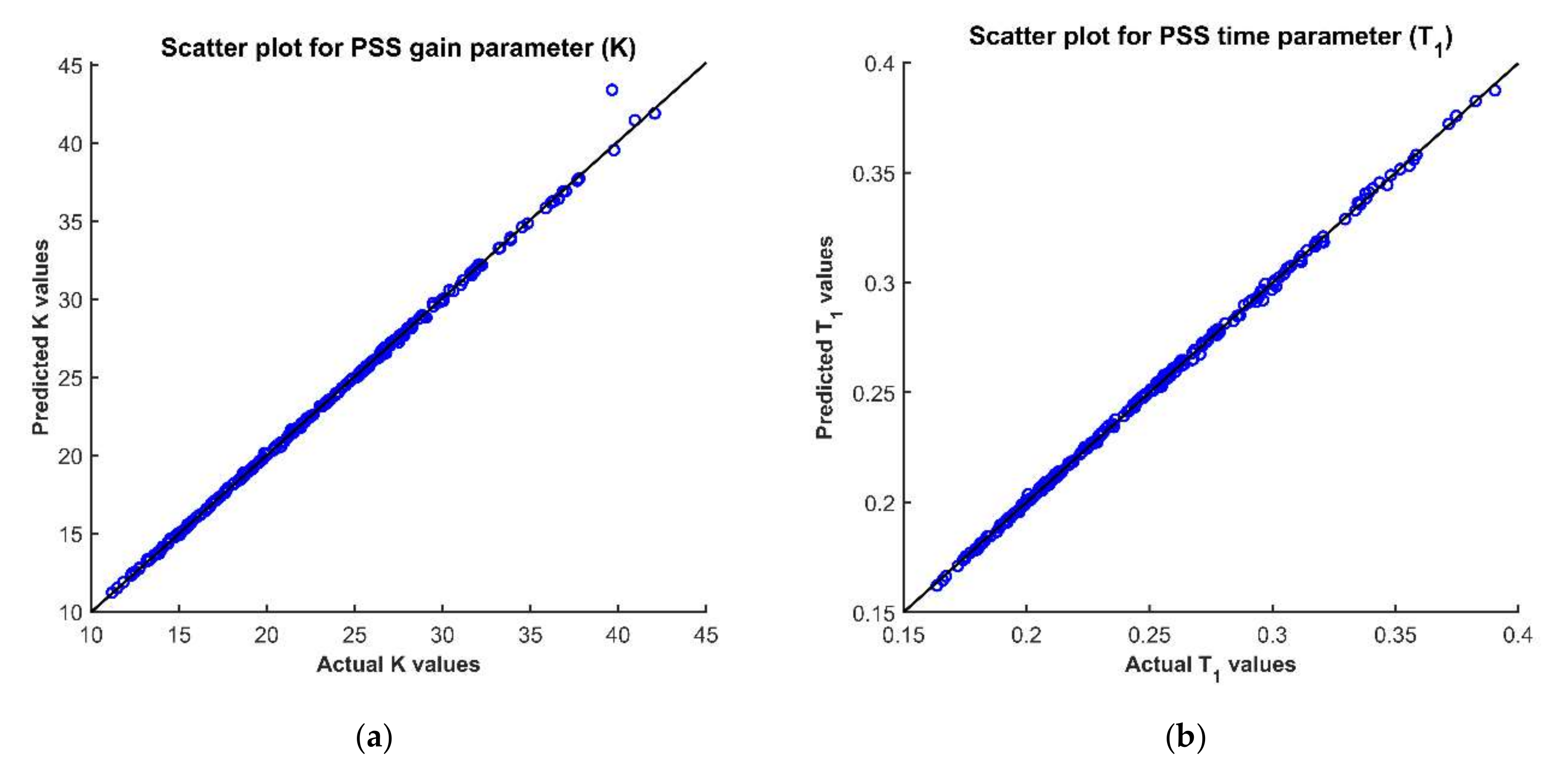
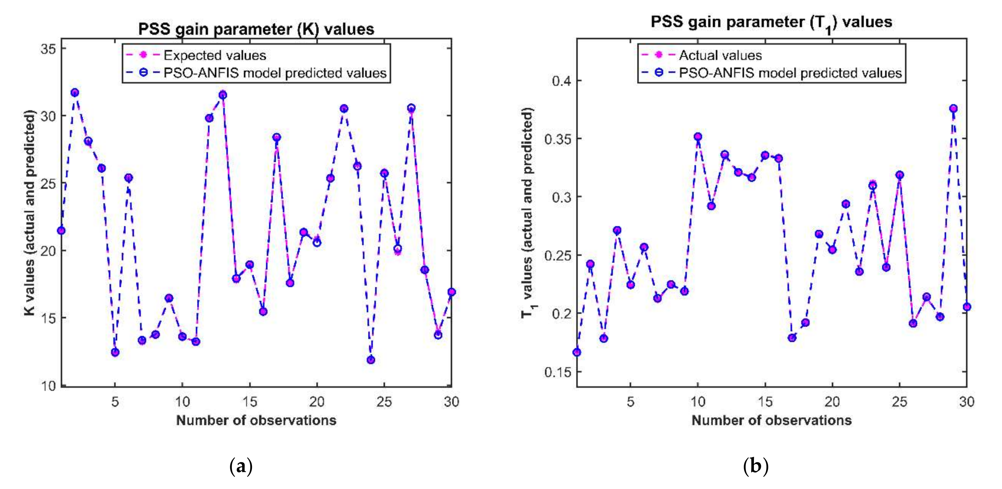
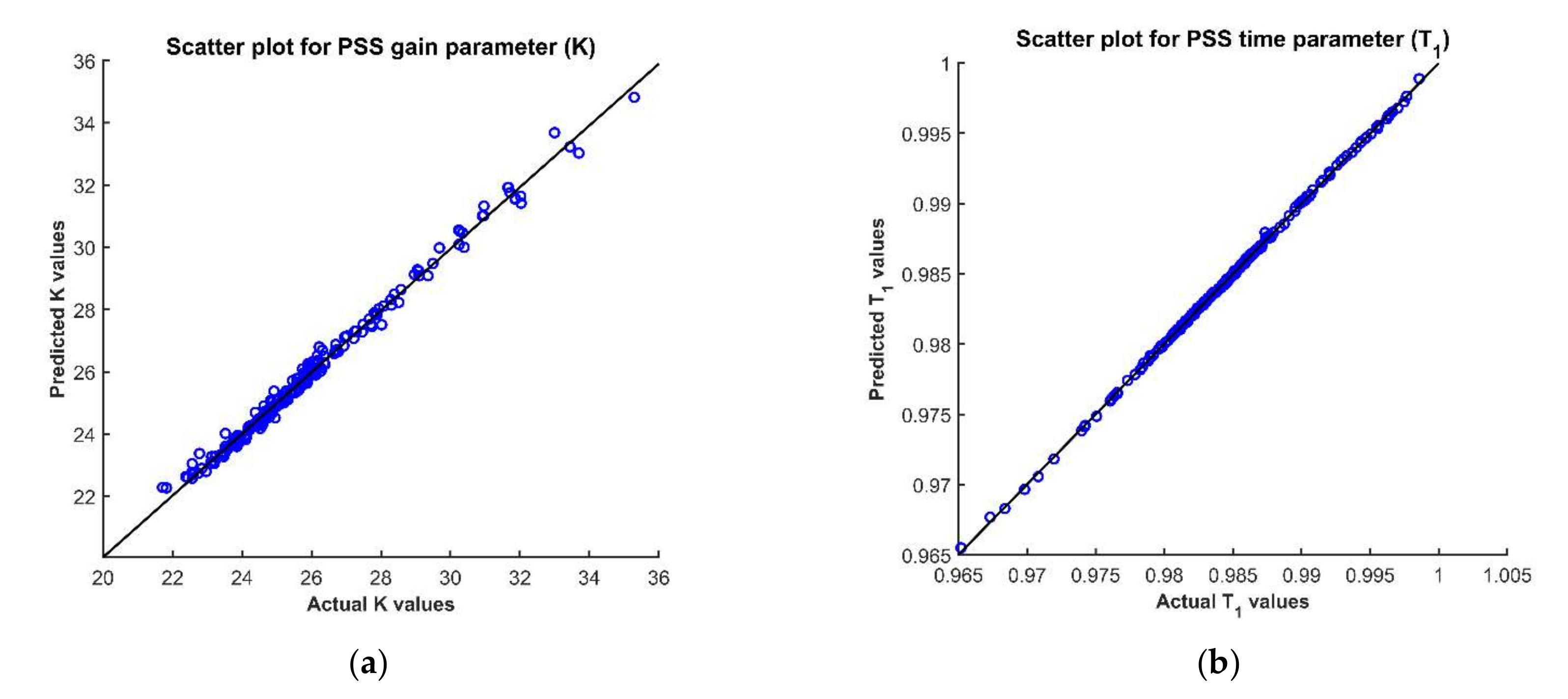
• The PSO inspired ANFIS model was developed by taking the range of operating points as the inputs and the PSS key parameters as the outputs. Different statistical parameters were used to check the efficacy of the developed model.
• The proposed ANFIS model was assessed to provide the optimal PSS parameter in real-time, under any loading condition. Time-domain analysis, eigenvalues, and the damping ratios were used to measure the developed approach’s performance.

The rest of the paper is organized as follows: Section 2 illustrates the dynamic models of electric networks under investigation. Section 3 presents the proposed machine learning (PSO inspired ANFIS) tool for real-time tuning of the PSS parameters. Section 4 demonstrates the proposed machine learning model development along with the data generation and processing technique. Section 5 offers a detailed discussion of the obtained results and the developed ML model’s compatibility and superiority. Finally, Section 6 provides concluding remarks along with the future research directions on the topic under investigation.

2. Power System Models

This article analyzed two different power system networks’ stability employing the proposed PSO-ANFIS tool by tuning the PSS parameters in real-time. This section briefly describes the modeling of these two networks under investigation.

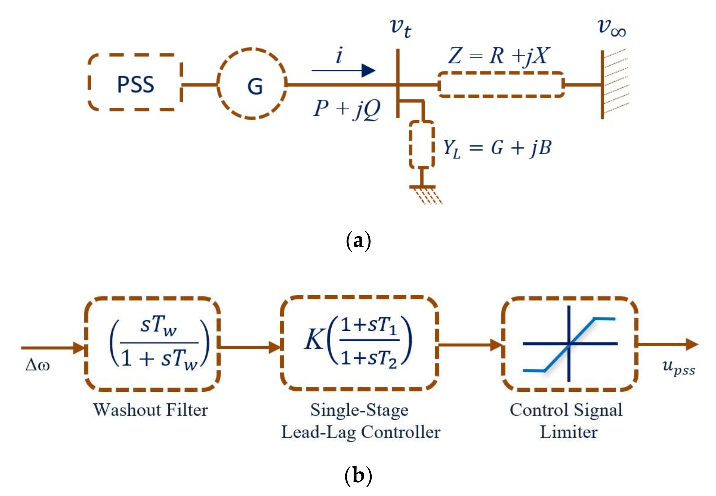
2.1. Example 1: SMIB Electric Network without UPFC

Figure 1a shows the PSS integrated SMIB electric power network, where the synchronous generator is connected to an infinite bus system through a transmission line of specific reactance. The fourth-order nonlinear model of the SMIB system and its linearized form can be found in [36,37,38,39]. The incorporated PSS is one of the commonly used single-stage lead-lag controllers, as shown in Figure 1b. The state-space model of the overall network after inclusion of the PSS is available in Ref. [36] and represented as (1) where the number of states is six.

$$\dot{X_1}=A_{c1}\Delta X_1$$

(1)

The modes of a power network are represented by the eigenvalues of its state matrix (Ac₁) corresponding to the system states. Any small disturbances on the system are reflected on the eigenvalues. The electric network’s stability is ensured if all the eigenvalues lie within the left half-plane of the complex plane, meaning real parts of the eigenvalues should take negative numbers. On the contrary, the positive real part of any one of the eigenvalues leads towards system instability. Therefore, appropriate tuning of the PSS parameters is the key to locate all the eigenvalues of the state matrix of the targeted electric network in the left half-plane that ensures the system stability. Additionally, proper placement of the eigenvalues on the complex plane enhances the system stability by suppressing the low-frequency oscillations. This article tuned the PSS parameters of the SMIB system employing the developed PSO-ANFIS tool where the inputs were the system operating conditions, e.g., terminal voltage, real power, and reactive power of the machine.

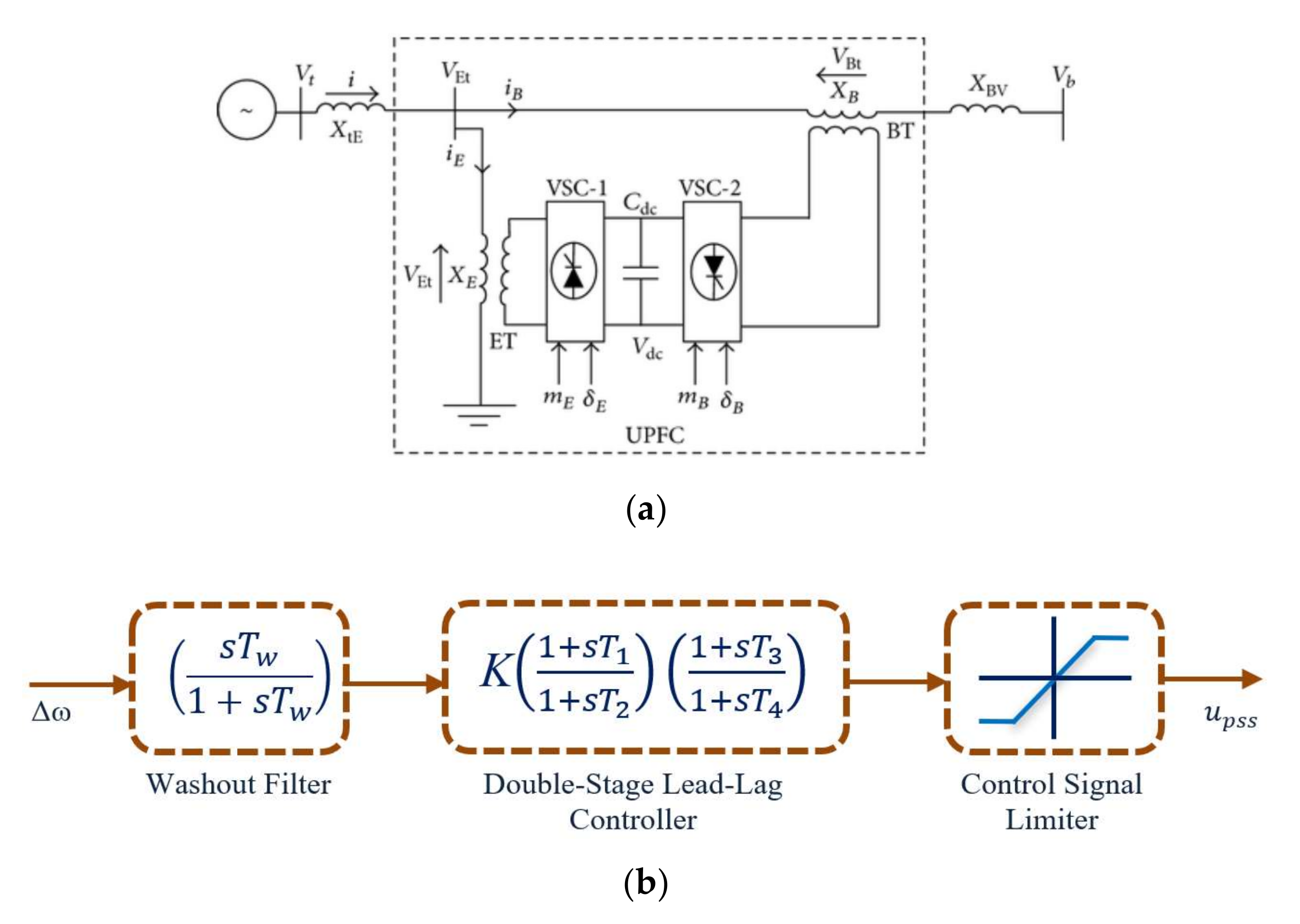
2.2. Example 2: SMIB Electric Network Equipped with PSS and UPFC

In the second test network, a SMIB system is equipped with a UPFC, as shown in Figure 2a, where the synchronous machine is connected with an infinite bus through a transmission line. In this case, a PSS is also connected with the synchronous machine and coordinated with the UPFC to improve the system stability. A boosting transformer (BT) and an excitation transformer (ET) link the UPFC with the network. With a voltage source converter (VSC-E) aid, a DC link capacitor is coupled with the ET. Likewise, the BT is coupled with that capacitor through another voltage source converter (VSC-B). The UPFC has a total of four control parameters consisting of two-phase angles and two-amplitude modulation ratios. Therefore, according to the specification in Figure 2a, the phase angles of boosting and excitation transformers are δ_B and δ_E. The amplitude modulation ratios of boosting and excitation transformers are m_B and m_E. A detailed explanation of these control parameters and the considered system can be found in [26,27,28,29]. The structure of a two-stage lead-lag PSS is shown in Figure 2b. Like the first network of Figure 1b, this two-stage lead-lag PSS is coupled with the synchronous generator and coordinated with the UPFC. After incorporating both the PSS and UPFC into the system and linearization, the final state-space model can be formulated, consisting of nine states. This overall model of the PSS-UPFC incorporated SMIB system can be represented by Equation (2) [36].

$$\dot{X_2}=A_{c2}\Delta X_2$$

(2)

As mentioned earlier, the state matrix’s eigenvalues (Ac₂) indicate the modes of operation of the system after being subjected to any disturbances. The electric network’s stability is ensured when all eigenvalues lie within the complex plane’s left half-side, meaning all eigenvalues should have negative real parts. On the other hand, the positive real part of anyone of the state matrix’s eigenvalues leads the system into instability. Therefore, the proper selection of PSS parameters is the key to placing the system eigenvalues in the left half-plane to enhances system stability by damping out the LFO. This article proposed a strategy to tune the UPFC coordinated PSS parameters of the SMIB system employing the PSO-ANFIS tool where the inputs were the system operating conditions.

3. Proposed Optimization Method

In this article, PSO optimized ANFIS models were employed to estimate the PSS parameters of the SMIB systems either incorporated the UPFC or functioning alone. The successful performance of ANFIS models depends on the appropriate parameter selection through rigorous training and testing processes. Both the derivative and metaheuristic-based approaches for selecting appropriate parameters of ANFIS can be found in [41]. In the following subsections, the ANFIS model and the PSO algorithm are described briefly.

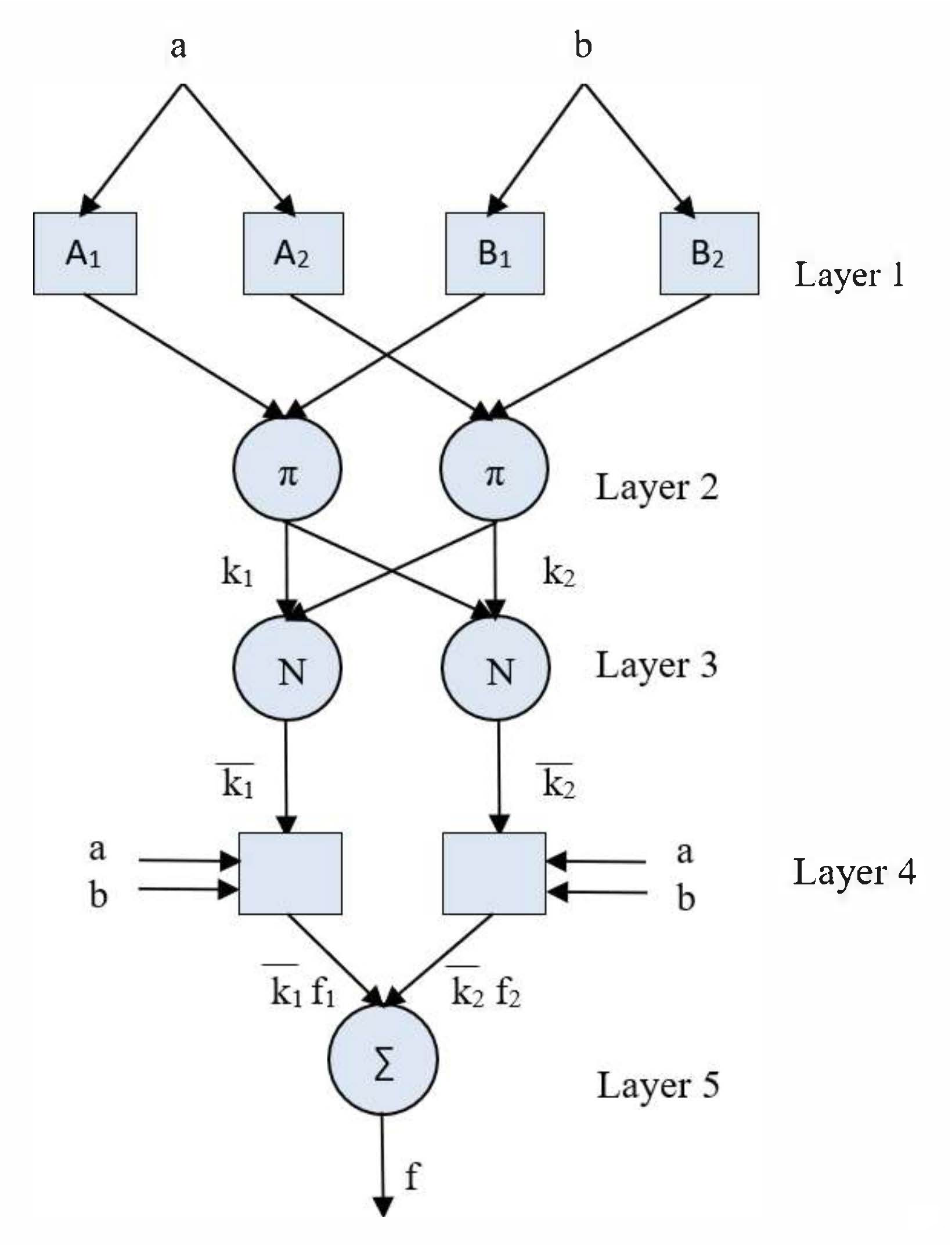
3.1. Adaptive Neuro-Fuzzy Inference System (ANFIS)

The ANFIS integrates the property of two machine learning algorithms: neural network and fuzzy logic. It was first proposed in 1993 [42] and demonstrated significant success in diverse application fields for its unique features [43,44]. It uses fuzzy logic to convert the given inputs to a targeted output, with the help of highly interconnected neural network processing elements. Figure 3 shows the basic structure of the ANFIS consisting of two inputs, one output, two membership functions, and two fuzzy rules that works in five different stages [41]. The first stage ($M_i^1$), also known as the fuzzification stage, obtains the fuzzy clusters from the provided inputs (a and b) through the membership functions. The premise parameters (x, y, and z) determine the nature of the membership function. The degree of membership, µA_i(a), can be calculated from the following Equation (3) for the first input. Similarly, it can be calculated for the second input as µB_i(b).

$$M_i^1= \mu A_i\left(a\right)=gbellm f\left(a;x,y,z\right)= \frac{1}{1+{\left|\frac{a-z}{x}\right|}^{2y}}$$

(3)

The next layer ($M_i^2$), also known as the rule layer, uses the membership values of the previous layer and calculates the firing strengths ($k_i$) of the applied rules by multiplying the membership values as in (4).

$$M_i^2= k_i=\mu A_i\left(a\right).\mu B_i\left(b\right) i=1, 2, \dots$$

(4)

The third layer ($M_i^3$), known as the normalization layer, calculates the normalized firing strengths (${\overline{k}}_l$) for all the applied rules. The normalization approach is shown below in (5), where the corresponding value of k is divided by the total firing strength.

$$M_i^3= {\overline{k}}_l=\frac{k_i}{k_1+k_2+k_3+k_4} i\in \left\{1, 2, 3, 4\right\}$$

(5)

In the next stage ($M_i^4$), defuzzification is performed, as shown in (6), where all the rules’ weighted values are found for each node. The first-order polynomial determines these values where $m_i$, $n_i$, and $o_i$ represent the coefficients. The number of coefficients, known as the consequence parameters, is one more than the given inputs.

$$M_i^4={\overline{k}}_l{f}_i={\overline{k}}_l\left(m_{i}a+n_{i}b + o_i\right)$$

(6)

Finally, the ANFIS model’s output is calculated in the fifth stage ($M_i^5$) by adding all the weighted outputs according to (7).

$$M_i^5={\displaystyle \sum }_i{\overline{k}}_l{f}_i=\frac{{{\displaystyle \sum }}_i{k}_i{f}_i}{{{\displaystyle \sum }}_i{k}_i}$$

(7)

The above-mentioned parameters of the ANFIS models are optimized using the PSO algorithm in this article through comprehensive training and testing processes.

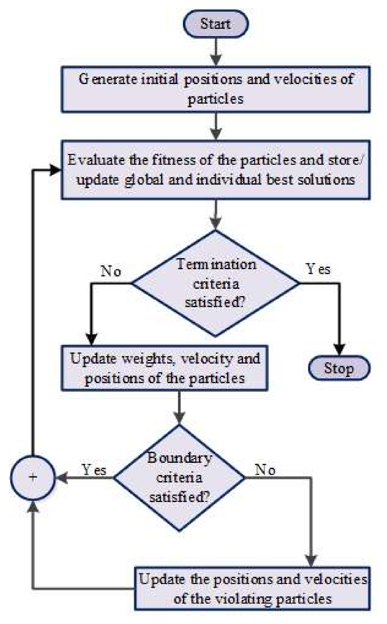
3.2. Particle Swarm Optimization (PSO)

The PSO, a swarm-based metaheuristic technique, is used to search the global solution from the search space. This optimization technique is inspired by biological populations’ swarming characteristics like a flock of birds or school of fishes that move together in the multi-directional search spaces to find the food source, inhabitation place, or other objectives. During this searching process, the swarm particles (birds/fishes) can change and adjust their movements and positions based on their social and cognitive experiences. Kennedy and Eberhart introduced this global search optimization algorithm in Ref. [45]. In PSO, every particle locates a position in the search space and continually changes its position to find the optimal location. Thus, the global solution can be exploited by any particle of the swarm. Initially, a random set of particles is assumed with a probable location of each particle, and the velocity of each particle within the swarm is also generated. The algorithm then evaluates the fitness of the particle’s positions based on the objective function of the optimization problem under investigation. The particles’ positions are stored as the individual best solutions and the best position as the global best solution. In each iteration, the PSO algorithm updates the inertia weight and velocities of the particles, hence the particles’ positions. The update of the particles’ velocities depends on three main factors: the inertia component, the cognitive component, and the social component. According to the PSO model proposed by Kennedy and Eberhart, each swarm particle’s new position is translated/enhanced from the old position with respect to the corresponding particle’s new velocity. A detailed explanation of the PSO algorithm model can be found in [46]. Hence, this procedure of updating the particles’ velocities and positions is repeated in each iteration until the targeted convergence criteria are satisfied. The flow diagram of the PSO algorithm is shown in Figure 4. According to this flow diagram, the initial positions and velocities are generated randomly, and after evaluation of their fitness, the individual and the global best solutions are stored. After that, if the stopping criteria are satisfied for the stored solutions, the algorithm is terminated; otherwise, the inertia weight, velocities, and positions of the swarm particles are updated again. Then, after checking the boundary violation condition, the particles’ positions’ fitness is evaluated, and the algorithm continues as illustrated in the flow diagram.

4. Data Processing and ANFIS Model Development

Details of data generation and processing and the ANFIS model development steps are illustrated in the following subsections.

4.1. Data Generation and Processing

In this research, a total of 1000 loading conditions for each of the considered power system networks from the ranges of operating conditions given in

Table 1. Ranges of the operating condition in per unit (pu) for the selected power system networks.

Limit	Real Power (Pe)	Reactive Power (Qe)	Terminal Voltage (Vt)
Minimum	0.40	−0.30	0.90
Maximum	1.10	0.40	1.10

were generated. These data sets were prepared with the variation and combination of three parameters of the power systems: terminal voltage (V_t), real power (P_e), and reactive power ($Q_e$). Each variety of selected parameters was considered as a distinct loading condition of the corresponding electric network. The PSO algorithm was then employed to optimize the PSS’s key parameters (K and T₁) in offline mode for all generated loading conditions. For the first network, the objective was to maximize the system minimum damping ratio. In contrast, the second network’s objective function was to minimize a multi-objective function combining two major decision-taking parameters, e.g., damping factor and damping ratio. Details about the optimization problem formulation and solution methodologies using the PSO can be found in [47] and in [48] for the first and second networks. As shown in Figure 5, the PSO algorithm converged the objective functions to the specific values for both networks for five different runs that signified the algorithm’s robustness and efficacy in finding PSS key parameters.

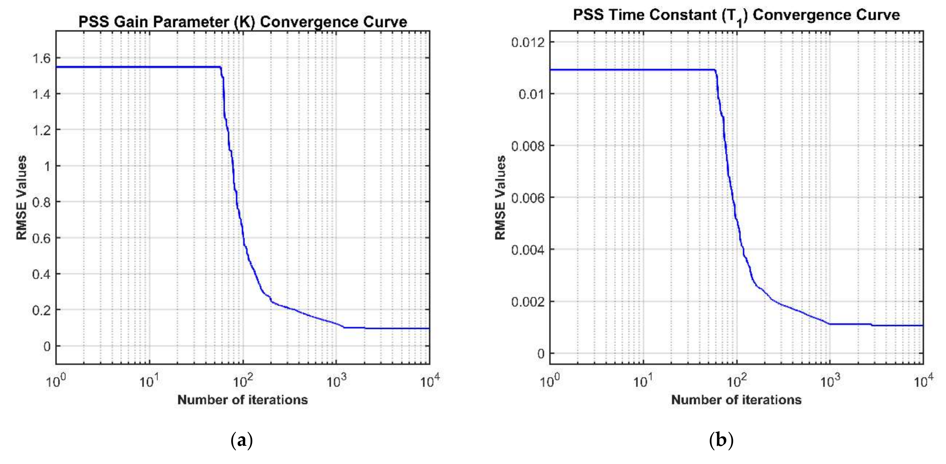
4.2. PSO-ANFIS Model Development

In this work, the ANFIS toolbox available in [49] was employed, where 70% of data were used for training, and 30% of data were used for the testing purposes of the proposed machine learning tool. A continually regulated trial and error process was taken into account to adjust the ANFIS models’ parameters. Statistical performance indices, including the RMSE, MAPE, RSR, R², and WIA, were measured to evaluate the proposed PSO-ANFIS models’ effectiveness in predicting PSS key parameters. The higher values of RMSE, MAPE, and RSR refer to more unsatisfactory model performance. On the contrary, the remaining indices, R² and WIA, maintain the unity values for perfect matching between the model predicted output and the actual system output. In contrast, the variation of R² and WIA values from “1” to “0” indicates matching the predicted and actual data from 100% to 0%. To investigate the efficiency of the proposed PSO-ANFIS models in predicting PSS key parameters, the mentioned SPI values were evaluated and summarized in Table 5 for both networks’ testing datasets.

Based on the obtained MAPE and R² values of

Table 2. Mean absolute percentage error (MAPE) and R² values with the different number of clusters for the ANFIS model (first test network).

Cluster Number	Gain Parameter (K)		Time Constant Parameter (T1)
	MAPE	R2	MAPE	R2
2	3.5455	0.9867	2.1450	0.9900
3	4.3358	0.9882	2.3695	0.9887
4	2.4405	0.9939	2.5640	0.9873
5	4.8319	0.9836	2.0364	0.9903
6	2.8576	0.9935	2.2844	0.9884
7	4.0036	0.9868	2.6272	0.9862
8	3.7293	0.9874	1.9038	0.9928
9	2.4318	0.9948	1.9486	0.9926
10	3.9331	0.9872	2.1869	0.9854
11	3.2829	0.9911	1.9155	0.9924
12	3.3876	0.9895	2.1047	0.9915

and

Table 3. MAPE and R² values with the different number of clusters for the ANFIS model (second test network).

Cluster Number	Gain Parameter (K)		Time Constant Parameter (T1)
	MAPE	R2	MAPE	R2
2	1.3557	0.9779	0.2414	0.8196
3	2.1198	0.9564	0.2667	0.7990
4	1.0857	0.9864	0.1834	0.8838
5	2.0702	0.9522	0.1039	0.9703
6	0.8781	0.9915	0.1213	0.9548
7	0.7446	0.9942	0.1376	0.9277
8	1.4883	0.9774	0.1553	0.9356
9	1.5006	0.9781	0.0786	0.9824
10	1.2636	0.9807	0.1255	0.9607
11	1.3736	0.9770	0.1305	0.9484
12	1.4426	0.9770	0.1304	0.9497

, this research selected 8 and 9 clusters for the first and second networks, respectively. The selected clusters were used to model the PSS key parameters (K and T₁). It is worth noting that it selected 10,000, 1, and 0.99 as the maximum number of iterations, inertia weight, and inertia weight damping ratio, respectively. The cognitive and social learning coefficients were selected as 1 and 2, respectively. The total numbers of parameters of the ANFIS models for the first and the second networks were 80 and 90, respectively, as per their preselected number of clusters. The particle positions corresponding to the ANFIS parameters to be optimized were found from the ‘GetFISParams’ function of the employed toolbox of Ref. [49]. In the ANFIS models, the parameters related to the input (fuzzification) and output (defuzzification) sides are known as the premise and the consequence parameters [41]. Out of the 80 parameters of the ANFIS models of the first electric network, 48 of them were the premise parameters, and the remaining 32 were the consequence parameters.

Similarly, there were 54 premise and 36 consequence parameters of ANFIS models of the second electric network.

Table 4. Optimized parameters of the ANFIS model for the second test network during tuning of Table 1. parameter.

#ID	Value	#ID	Value	#ID	Value	#ID	Value	#ID	Value	#ID	Value
1	0.0912	16	0.9188	31	0.0841	46	25.1397	61	0.0215	76	0.0742
2	0.7817	17	−1.8641	32	0.0125	47	0.0235	62	0.9653	77	0.0230
3	0.0919	18	18.7428	33	0.0822	48	0.9688	63	0.0247	78	0.9509
4	0.7248	19	0.0799	34	0.7026	49	0.0238	64	0.4873	79	−0.0283
5	0.1297	20	−0.1893	35	−2.1530	50	0.9967	65	−0.5668	80	0.0102
6	0.4261	21	0.0835	36	4.9097	51	0.0308	66	6.0841	81	0.0159
7	0.0994	22	−0.1487	37	0.0237	52	1.0634	67	−0.0078	82	0.9918
8	0.5793	23	−2.1377	38	0.9641	53	−0.3098	68	0.0228	83	−0.0069
9	−0.4695	24	−1.0173	39	0.0233	54	24.8816	69	0.0219	84	0.0181
10	−18.226	25	0.0832	40	0.9745	55	0.0026	70	0.9659	85	0.0208
11	0.0987	26	−0.0634	41	−0.0309	56	−0.0072	71	−0.0717	86	0.9667
12	0.7177	27	−2.1694	42	1.3100	57	0.0218	72	0.1264	87	0.1009
13	0.1114	28	1.3801	43	0.0235	58	0.9682	73	−0.2241	88	−0.2637
14	0.3909	29	0.0810	44	0.9856	59	−0.0049	74	3.6773	89	0.0768
15	0.0294	30	−0.1725	45	0.0525	60	0.0149	75	0.0033	90	−24.141

presents the optimized parameters of the ANFIS model while tuning the T₁ parameter of the second electric network. Moreover, to set the PSO algorithm-generated values of the premise and consequence parameters, the ‘SetFISParams’ function inside the ‘TrainFISCost’ of the toolbox was employed. However, as can be seen from

Table 5. Test datasets statistical performance indices (SPI) values of the developed PSO-ANFIS models for both networks.

Parameter		RMSE	MAPE	RSR	PIBIAS	R2	WIA
K	First network	0.2640	0.0032	0.0401	−0.0736	0.9992	0.9996
	Second network	0.2003	0.0058	0.0853	0.0539	0.9964	0.9982
T1	First network	0.0011	0.0032	0.0219	0.0248	0.9998	0.9999
	Second network	0.0001	0.0001	0.0187	−0.0004	0.9998	0.9999

, the SPI indices, RMSE, MAPE, and RSR values are minimal, while the other two SPI indices’ values are close to unity for both electric networks. Furthermore, the MAPE and R² were improved significantly with the PSO optimized ANFIS model over the nonoptimized ANFIS model for both test networks (comparison of Table 2, Table 3 and Table 5). Therefore, SPI’s obtained values confirmed the proposed PSO tuned ANFIS models’ effectiveness in estimating PSS parameters.

Figure 6 and Figure 7 show the RMSE values convergence curves, and the scatter plots for the PSS key parameters (K and T₁) of the first network test dataset. Figure 8 shows the expected and approximated gain parameter (K) and time constant parameter (T₁) values for randomly chosen thirty different operating/loading conditions from the first electric network’s test dataset. In this case, the actual values were evaluated using the offline mode PSO algorithm, whereas the estimated ones were the output from the PSO-ANFIS model. It can be observed from Figure 8 that the predicted and actual values of the PSS parameters (K and T₁) are entirely overlapped with each other. Therefore, the proposed PSO-ANFIS model showed confidence in the online estimation of the first electric network’s PSS parameters. Likewise, Figure 9 and Figure 10 show the RMSE values convergence curves, and the scatter plots for the UPFC coordinated PSS key parameters (K and T₁) of the second network test dataset. Furthermore, Figure 11 proved the efficiency of estimating the PSS parameters employing the proposed PSO-ANFIS learning model for the second electric network. Therefore, Figure 6 to Figure 11 confirmed the developed PSO-ANFIS models’ effectiveness in predicting PSS key parameters for both electric networks.

Lastly, it is essential to mention that this research was carried out using the MATLAB simulation environment in a desktop computer with an Intel Core i5 (3.5 GHz Processors, 8 GB RAM). It required several hours to develop the PSO-ANFIS models. However, the developed PSO-ANFIS models estimated the first network’s PSS parameters around 0.285 s for 700 arbitrarily produced operating situations. Hence, the proposed model required an average of around 0.000407 s to estimate the PSS parameters for a single operating situation. For the second test system, the developed PSO-ANFIS models took 0.30 s to estimate UPFC coordinated PSS parameters for another 700 loading conditions; thus, it required an average of 0.000429 s for a single loading condition. As mentioned, the times needed for PSS parameters estimation employing the developed PSO-ANFIS models are almost 35 times smaller than a period of 60 Hz electric network. Therefore, a conclusion can be made that the faster response of the developed PSO-ANFIS models makes them suitable to be implemented online in tuning the PSS parameters.

5. Results and Discussion

It is already mentioned that this paper proposed the PSO-ANFIS models that were applied to two different electric networks to estimate the PSS key parameters in real-time. In this section, the proposed ANFIS models’ effectiveness was examined based on eigenvalues and minimum damping ratio for both systems under investigation. The efficacy of the developed models was also justified in online implementation through time-domain simulation results for some specific states of the machine.

5.1. Example 1: SMIB Electric Network with PSS only

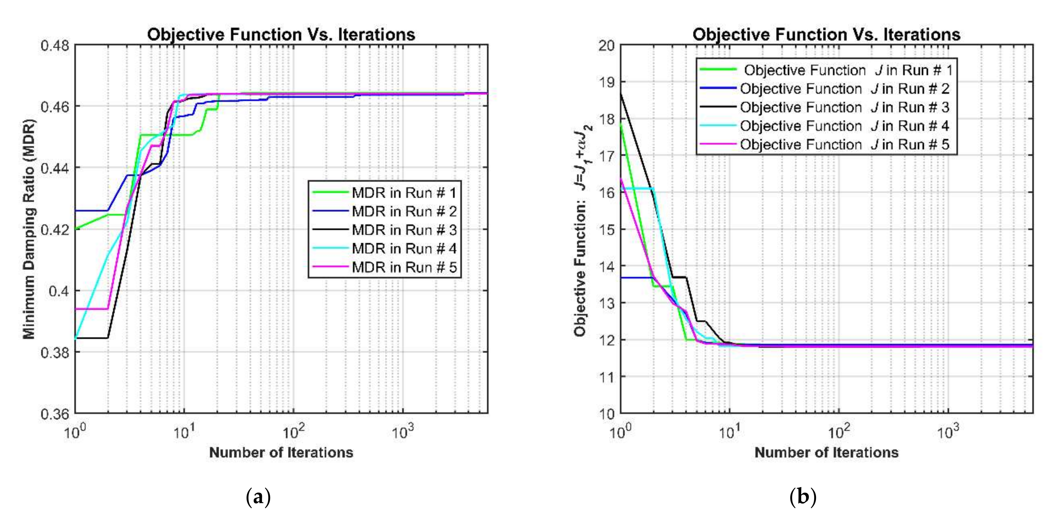
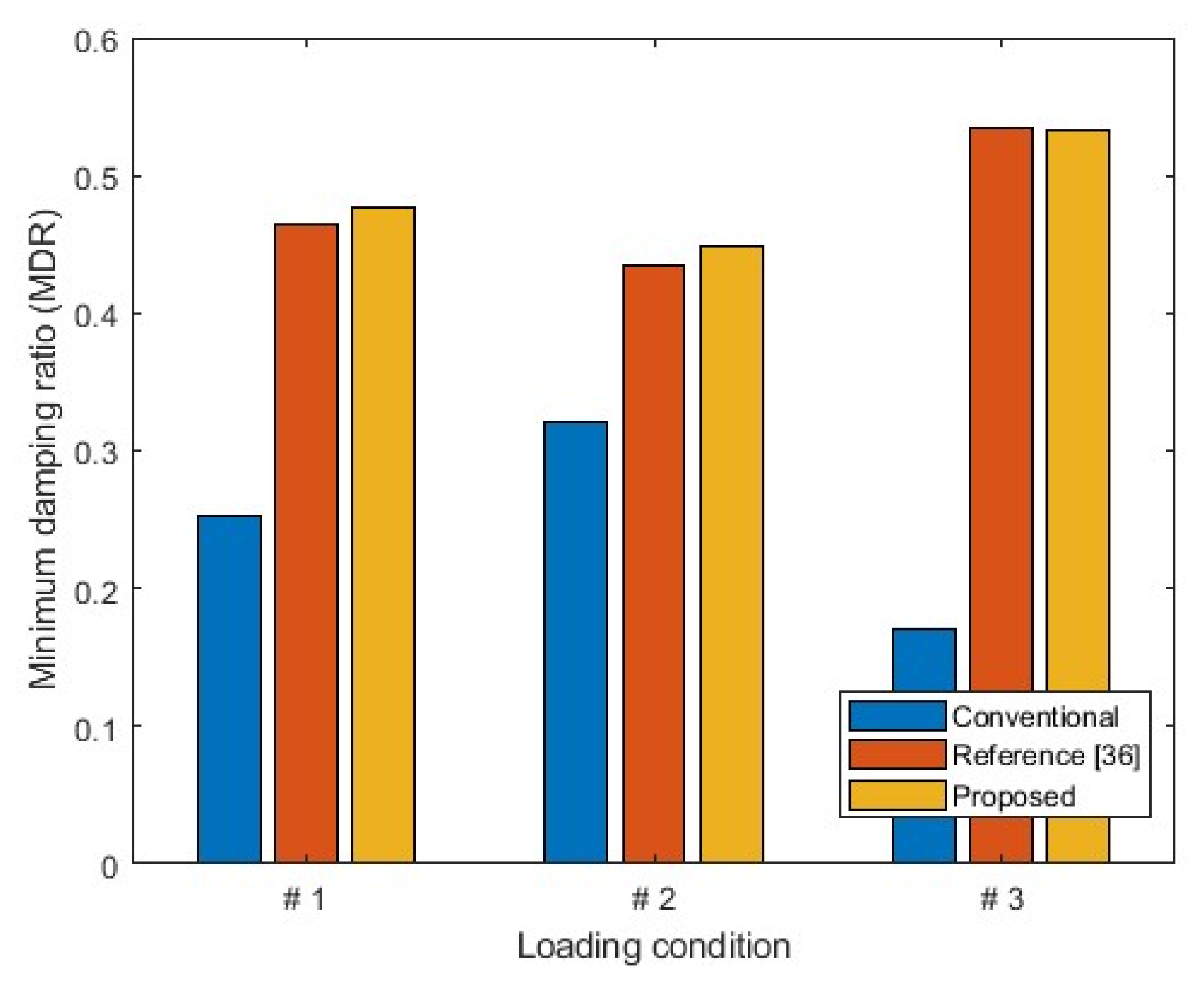
5.1.1. Eigenvalues and Minimum Damping Ratio Analyses

Estimated PSS key parameters using the developed PSO-ANFIS model for three different operating conditions of the first test network were evaluated and summarized in

Table 6. Estimated PSS key parameters using the developed PSO-ANFIS models for three different operating situations (first network).

Case	Pe (pu)	Qe (pu)	Vt (pu)	Gain Parameter (K)		Time Constant Parameter (T1)
				PSO-ANFIS	Conventional	PSO-ANFIS	Conventional
Loading condition # 1	1.000	0.015	1.050	18.365	7.090	0.263	0.685
Loading condition # 2	0.894	−0.281	0.955	13.526		0.325
Loading condition # 3	0.955	0.276	1.031	25.639		0.194

. Corresponding eigenvalues and minimum damping ratio values of the loading conditions of Table 6 were presented in

Table 7. Eigenvalues and MDR comparison for the operating situation # 1 (first network).

Item	Conventional PSS	Ref. [37]	Proposed
Eigenvalues	−0.337	−0.346	−0.346
	−18.703 1.127 ± j4.333 −4.4618 ± j7.483	−18.207 −2.982 ± j5.6949 −3.006 ± j5.342	−18.206 −2.928 ± j5.386 −3.061 ± j5.653
MDR	0.252	0.464	0.476

,

Table 8. Eigenvalues and MDR comparison for the operating situation # 2 (first network).

Item	Conventional PSS	Ref. [37]	Proposed
Eigenvalues	−0.337	Not available	−0.342
	−19.123 −1.494 ± j4.408 −4.040 ± j7.551		−18.508 −2.801 ± j5.583 −3.038 ± j5.676
MDR	0.3209	0.464	0.448

, and

Table 9. Eigenvalues and MDR comparison for the operating situation # 3 (first network).

Item	Conventional PSS	Ref. [37]	Proposed
Eigenvalues	−0.338	Not available	−0.358
	−18.379 −0.621 ± j3.596 −5.285 ± j7.414		−17.673 −2.968 ± j4.709 −3.281 ± j4.927
MDR	0.170	0.534	0.533

. In this case, the eigenvalues in the tables for three cases were accumulated, including the PSO-ANFIS, conventional, and literature reported models with the same operating conditions for comparison purposes. As mentioned earlier, the eigenvalues’ positions within the left-side of the complex plane ensure the electric network’s stable operation. It is visible from the tables that the presented eigenvalues were situated in the left half-plane for all mentioned approaches. However, the PSO-ANFIS models showed effective action on the electric network in placing the eigenvalues at better positions over the conventional one. Furthermore, both referenced and developed models maintained higher MDR values than the conventional model. This higher MDR value ensured the developed model’s efficacy in damping out the LFO and gaining better stability of the developed model over the conventional one. Comparison of MDR values of the first electric network for three different loading conditions is shown in Figure 12.

5.1.2. Time-Domain Simulation under Disturbance

This section analyzed the performance of the PSO-ANFIS and the conventional models in damping out the LFO from the first electric system following an external disturbance. In this case, a pulse of an extra 10% of mechanical torque was introduced as a disturbance to the input at 1.0 s for four cycles. Following this disturbance, this research measured the responses of the two states (rotor angle and angular frequency) of the system. These responses (changes of rotor angle and angular frequency) of the synchronous machine were plotted in Figure 13a,b with the loading condition # 3 of Table 6. Although both models stabilized the electric network by damping out the LFO from the system, the PSO-ANFIS model demonstrated a faster response than the conventional one. From both figures, it can be observed that the developed PSO-ANFIS models damped out the LFO and stabilized the system states within 3.5 s, while the conventional model took approximately 6.0 s. Hence, it can be concluded that the developed PSO-ANFIS technique will be well-suited for real-time prediction of PSS parameters to damp out the LFO in the power system network.

5.2. Example 2: SMIB System with UPFC Coordinated PSS

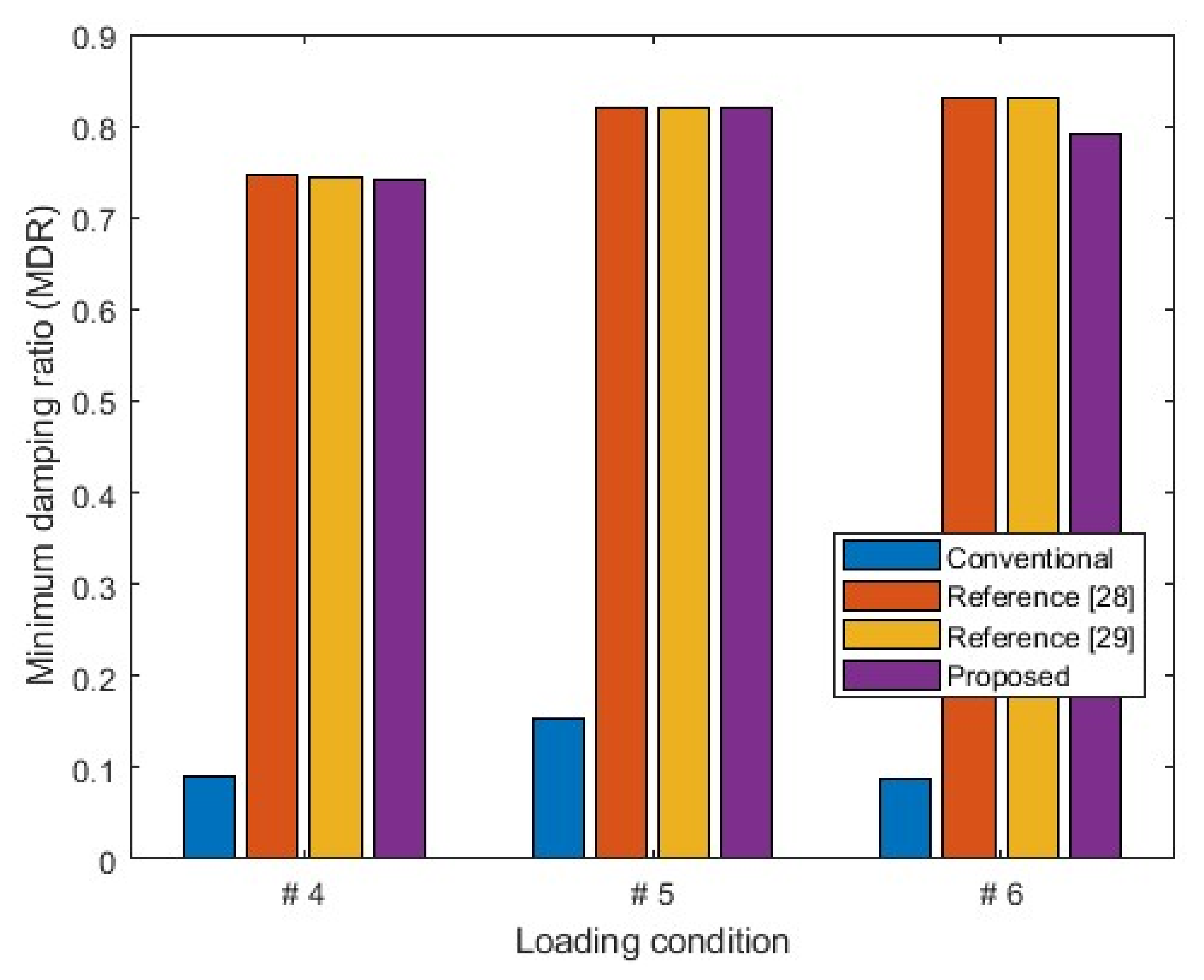
5.2.1. Eigenvalues and Minimum Damping Ratio Analysis

Estimated PSS key parameters using the developed PSO-ANFIS models for three different loading situations for the second test network were evaluated and summarized in

Table 10. Estimated PSS key parameters using the developed PSO-ANFIS models for three different operating situations (second network).

Case	Pe (pu)	Qe (pu)	Vt (pu)	Gain Parameter (K)		Time Constant Parameter (T1)
				PSO-ANFIS	Conventional	PSO-ANFIS	Conventional
Loading condition # 4	0.980	−0.160	1.000	24.005	15.000	0.984	0.500
Loading condition # 5	0.600	0.010	0.980	25.583		0.9839
Loading condition # 6	1.300	0.400	1.060	31.873		0.986

.

Table 11. Eigenvalues and MDR comparison for the operating situation # 4 (second network).

Item	Conventional PSS	Ref. [28]	Ref. [29]	Proposed
Eigenvalues	−0.206 −6.695 −86.497 −110.705 −994.471 −0.419 ± j4.610 −0.676 ± j0.320	−0.199 −1.056 −80.726 −125.389 −982.089 −1.493 ± j0.438 −4.159 ± j3.708	−0.199 −1.184 −80.7544 −125.298 −982.175 −1.459 ± j0.249 −4.118 ± j3.699	−0.199 −1.683 −80.806 −125.131 −982.332 −1.248 ± j0.136 −4.059 ± j3.673
MDR	0.091	0.746	0.744	0.741

,

Table 12. Eigenvalues and MDR comparison for the operating situation # 5 (second network).

Item	Conventional PSS	Ref. [28]	Ref. [29]	Proposed
Eigenvalues	−0.400 −6.593 −87.562 −110.031 −993.512 −0.615 ± j3.969 −0.718 ± j0.295	−0.391 −1.089 −83.489 −126.897 −977.786 −1.463 ± j0.302 −4.092 ± j2.851	−0.391 −1.203 −83.489 −126.899 −977.784 −1.415 ± j0.160 −4.084 ± j2.853	−0.391 −1.466 −83.494 −126.867 −1.291 ± j0.078 −977.816 −4.0744 ± j2.847
MDR	0.153	0.821	0.820	0.820

, and

Table 13. Eigenvalues and MDR comparison for the operating situation # 6 (second network).

Item	Conventional PSS	Ref. [28]	Ref. [29]	Proposed
Eigenvalues	−0.147 −7.269 −87.048 −112.996 −991.096 −0.427 ± j4.801 −0.677 ± j0.274	−0.143 −1.936 −82.539 −136.569 −967.917 −1.1471 ± j0.169 −4.683 ± j3.141	−0.143 −2.025 −82.571 −136.306 −968.192 −1.141 ± j0.128 −4.623 ± j3.107	−0.141 −1.063 −81.860 −142.793 −961.396 −1.009 ± j0.781 −5.746 ± j3.741
MDR	0.089	0.831	0.830	0.791

tabulated the corresponding eigenvalues and MDR values. The tables also accumulated the eigenvalues and MDR values of the literature reported and the conventional models for the same loading conditions for comparison purposes. All models of the tables exhibited stable operation as the eigenvalues were placed on the left half-plane. However, the PSO-ANFIS models demonstrated better stability over the conventional one as the corresponding eigenvalues were located comparatively far away from the imaginary axis. Additionally, the PSO-ANFIS and the referenced works models maintained the larger MDR values over the conventional model that signified their abilities in damping out of the LFO to gain better stability. The comparison of the second test network’s MDR values for three different loading conditions is shown in Figure 14.

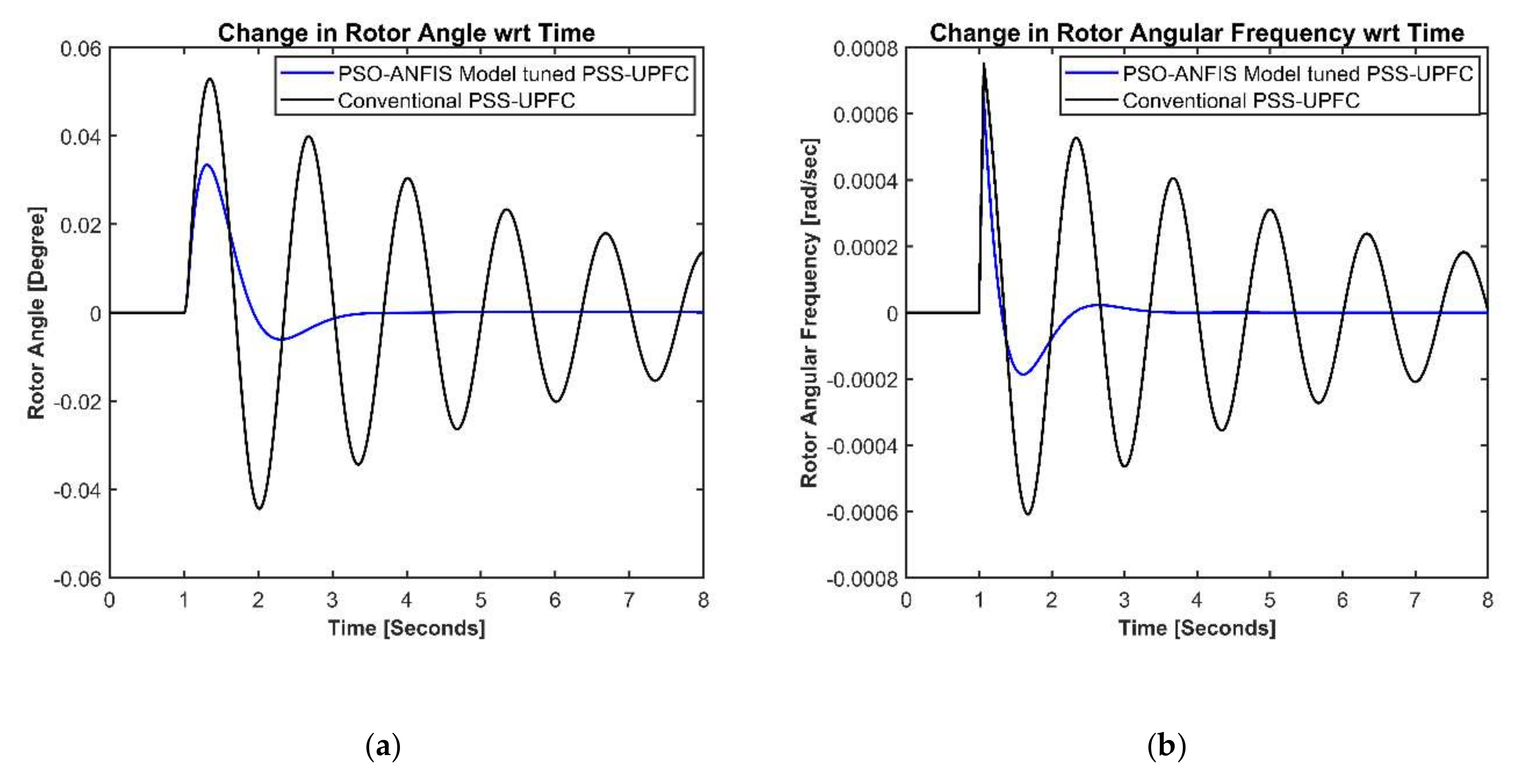
5.2.2. Time-Domain Simulation under Disturbance

Like the first electric network, this section analyzed the performance of the proposed PSO-ANFIS and the conventional models in damping out the LFO from the second test network following an external disturbance. A pulse of an extra 10% of mechanical torque was introduced again as a disturbance to the input at 1.0 s for four cycles. Following the disturbance, this research recorded the responses of the two states of the second electric network for the PSO-ANFIS and the conventional models. The recorded responses (changes in rotor angle and angular frequency) were plotted in Figure 15a,b for the loading condition # 4 of Table 10. As can be observed, both models stabilized the electric network by damping out the LFO from the system. However, the PSO-ANFIS models exhibited a faster response than the conventional one. The PSO-ANFIS models stabilized the power system’s states within 3.5 s, while the conventional method fails to damp out the LFO from the system even after 7.0 s. Hence, it can be concluded that the developed PSO-ANFIS technique demonstrated better suitability in improving the power system stability in real-time.

6. Conclusions

This paper proposed the PSO optimized ANFIS models for real-time (online) tuning of the PSS parameters to damp out the unwanted LFO from the electric power system networks. To evaluate the real-time operating performance, this research implemented the developed models on two different power system networks, namely the SMIB system with PSS only and the SMIB system with UPFC coordinated PSS. Then, it investigated the performance of the developed models for real-time power system stability enhancement. Superiority and compatibility of the developed models with the conventional and the referenced works were determined through eigenvalues and MDR values analyses for several operating situations. Additionally, the time-domain simulation results confirmed the superiority of the developed models over the conventional models for both test networks to damp out the LFO within reasonable times. The SPI’s fair values, including the RMSE, MAPE, RSR, R², and WIA, signified the developed PSO-ANFIS models’ effectiveness in predicting the PSS key parameters. Furthermore, it also notified that the required time for the developed models in estimating the PSS parameters was around 35 times less than that of a single cycle of 60 Hz electric network for any operating situation. Therefore, it can be concluded that the proposed PSO-ANFIS models have a high potentiality of deployment in electric grids for fine-tuning of the PSS parameters in real-time for system stability enhancement via damping out of the unwanted LFO. However, the proposed strategy’s robustness can be tested on other power system networks as the extension of this work, especially with multi-machine power system networks.

References

1. Kundur, P. Power System Stability and Control; McGraw-Hill: New York, NY, USA, 1994. [Google Scholar]
2. Bhukya, J.; Mahajan, V. Optimization of damping controller for PSS and SSSC to improve stability of interconnected system with DFIG based wind farm. Int. J. Electr. Power Energy Syst. 2019, 108, 314–335. [Google Scholar] [CrossRef]
3. Sambariya, D.K.; Prasad, R. Design of PSS for SMIB system using robust fast output sampling feedback technique. In Proceedings of the 2013 7th International Conference on Intelligent Systems and Control (ISCO), Coimbatore, India, 4–5 January 2013; pp. 166–171. [Google Scholar]
4. Jolfaei, M.G.; Sharaf, A.M.; Shariatmadar, S.M.; Poudeh, M.B. A hybrid PSS–SSSC GA-stabilization scheme for damping power system small signal oscillations. Int. J. Electr. Power Energy Syst. 2016, 75, 337–344. [Google Scholar] [CrossRef]
5. Assi Obaid, Z.; Cipcigan, L.M.; Muhssin, M.T. Power system oscillations and control: Classifications and PSSs’ design methods: A review. Renew. Sustain. Energy Rev. 2017, 79, 839–849. [Google Scholar] [CrossRef]
6. Eslami, M.; Shareef, H.; Mohamed, A. Application of PSS and FACTS Devices for Intensification of Power System Stability. Int. Rev. Electr. Eng. 2010, 5. [Google Scholar]
7. Alam, M.S.; Razzak, M.A.; Shafiullah, M.; Chowdhury, A.H. Application of TCSC and SVC in damping oscillations in Bangladesh Power System. In Proceedings of the 2012 7th International Conference on Electrical and Computer Engineering, Dhaka, Bangladesh, 20–22 December 2012; pp. 571–574. [Google Scholar]
8. Alam, M.S.; Shafiullah, M.; Hossain, M.I.; Hasan, M.N. Enhancement of power system damping employing TCSC with genetic algorithm based controller design. Int. Conf. Electr. Eng. Inf. Commun. Tech. 2015, 1–5. [Google Scholar]
9. Siddiqui, A.S.; Khan, M.T.; Iqbal, F. Determination of optimal location of TCSC and STATCOM for congestion management in deregulated power system. Int. J. Syst. Assur. Eng. Manag. 2017, 8, 110–117. [Google Scholar] [CrossRef]
10. Alizadeh, M.; Tofighi, M. Full-adaptive THEN-part equipped fuzzy wavelet neural controller design of FACTS devices to suppress inter-area oscillations. Neurocomputing 2013, 118, 157–170. [Google Scholar] [CrossRef]
11. Inkollu, S.R.; Kota, V.R. Optimal setting of FACTS devices for voltage stability improvement using PSO adaptive GSA hybrid algorithm. Eng. Sci. Technol. Int. J. 2016, 19, 1166–1176. [Google Scholar] [CrossRef] [Green Version]
12. Prasad, D.; Mukherjee, V. A novel symbiotic organisms search algorithm for optimal power flow of power system with FACTS devices. Eng. Sci. Technol. Int. J. 2016, 19, 79–89. [Google Scholar] [CrossRef] [Green Version]
13. Mukherjee, A.; Mukherjee, V. Chaotic krill herd algorithm for optimal reactive power dispatch considering FACTS devices. Appl. Soft Comput. 2016, 44, 163–190. [Google Scholar] [CrossRef]
14. Khan, M.T.; Siddiqui, A.S. FACTS device control strategy using PMU. Perspect. Sci. 2016, 8, 730–732. [Google Scholar] [CrossRef] [Green Version]
15. Wang, H.F. Applications of modelling UPFC into multi-machine power systems. IEE Proc. Gener. Transm. Distrib. 1999, 146, 306. [Google Scholar] [CrossRef]
16. Made Wartana, I.; Singh, J.G.; Ongsakul, W.; Buayai, K.; Sreedharan, S. Optimal placement of UPFC for maximizing system loadability and minimize active power losses by NSGA-II. In Proceedings of the 2011 International Conference and Utility Exhibition on Power and Energy Systems: Issues and Prospects for Asia, ICUE, Pattaya City, Thailand, 28–30 September 2011. [Google Scholar]
17. Elgamal, M.E.; Lotfy, A.; Ali, G.E.M. Voltage profile enhancement by fuzzy controlled MLI UPFC. Int. J. Electr. Power Energy Syst. 2012, 34, 10–18. [Google Scholar] [CrossRef]
18. Abdalla, A.A.; Ahmad, S.S.; Elamin, I.M.; Mahdi, M.A. Application of optimization algorithms for the improvement of the transient stability of SMIB integrated with SSSC controller. In Proceedings of the 2019 International Conference on Computer, Control, Electrical, and Electronics Engineering (ICCCEEE), Khartoum, Sudan, 21–23 September 2019. [Google Scholar]
19. Parkh, K.; Agarwal, V. Stability Improvement of SMIB System using TLBO Technique. In Proceedings of the 2019 3rd International Conference on Recent Developments in Control, Automation & Power Engineering (RDCAPE), Noida, India, 10–11 October 2019; pp. 323–328. [Google Scholar]
20. Hussain, A.N.; Hamdan Shri, S. Damping Improvement by Using Optimal Coordinated Design Based on PSS and TCSC Device. In Proceedings of the 2018 Third Scientific Conference of Electrical Engineering (SCEE), Baghdad, Iraq, 19–20 December 2018; pp. 116–121. [Google Scholar]
21. Khodabakhshian, A.; Esmaili, M.R.; Bornapour, M. Optimal coordinated design of UPFC and PSS for improving power system performance by using multi-objective water cycle algorithm. Int. J. Electr. Power Energy Syst. 2016, 83, 124–133. [Google Scholar] [CrossRef]
22. Hassan, L.H.; Moghavvemi, M.; Almurib, H.A.F.; Muttaqi, K.M. A Coordinated Design of PSSs and UPFC-based Stabilizer Using Genetic Algorithm. IEEE Trans. Ind. Appl. 2014, 50, 2957–2966. [Google Scholar] [CrossRef]
23. Shafiullah, M.; Rana, M.J.; Coelho, L.S.; Abido, M.A. Power system stability enhancement by designing optimal PSS employing backtracking search algorithm. In Proceedings of the 2017 6th International Conference on Clean Electrical Power (ICCEP), Santa Margherita Ligure, Italy, 27–29 June 2017; pp. 712–719. [Google Scholar]
24. Shahriar, M.S.; Shafiullah, M.; Asif, M.A.; Hasan, M.M.; Rafiuzzaman, M. Design of multi-objective UPFC employing backtracking search algorithm for enhancement of power system stability. In Proceedings of the 2015 18th International Conference on Computer and Information Technology ICCIT, Dhaka, Bangladesh, 22–23 December 2015; 2016; pp. 323–328. [Google Scholar]
25. Abido, M.A.; Al-Awami, A.T.; Abdel-Magid, Y.L. Analysis and design of UPFC damping stabilizers for power system stability enhancement. In Proceedings of the IEEE International Symposium on Industrial Electronics, Montreal, QC, Canada, 9–13 July 2006; Volume 3, pp. 2040–2045. [Google Scholar]
26. Vanitila, R.; Sudhakaran, M. Differential Evolution algorithm based Weighted Additive FGA approach for optimal power flow using muti-type FACTS devices. In Proceedings of the 2012 International Conference on Emerging Trends in Electrical Engineering and Energy Management (ICETEEEM), Chennai, India, 13–15 December 2012; pp. 198–204. [Google Scholar]
27. Shahriar, M.S.; Shafiullah, M.; Rana, M.J. Stability enhancement of PSS-UPFC installed power system by support vector regression. Electr. Eng. 2017, 1–12. [Google Scholar] [CrossRef]
28. Rana, M.J.; Shahriar, M.S.; Shafiullah, M. Levenberg–Marquardt neural network to estimate UPFC-coordinated PSS parameters to enhance power system stability. Neural Comput. Appl. 2019, 31, 1237–1248. [Google Scholar] [CrossRef]
29. Shafiullah, M.; Rana, M.J.; Shahriar, M.S.; Zahir, M.H. Low-frequency oscillation damping in the electric network through the optimal design of UPFC coordinated PSS employing MGGP. Measurement 2019, 138, 118–131. [Google Scholar] [CrossRef]
30. Shafiullah, M.; Rana, M.J.; Shahriar, M.S.; Al-Sulaiman, F.A.; Ahmed, S.D.; Ali, A. Extreme learning machine for real-time damping of LFO in power system networks. Electr. Eng. 2020, 1, 3. [Google Scholar] [CrossRef]
31. Shafiullah, M.; Khan, M.A.M.; Ahmed, S.D. PQ disturbance detection and classification combining advanced signal processing and machine learning tools. In Power Quality in Modern Power Systems; Sanjeevikumar, P., Sharmeela, C., Holm-Nielsen, J.B., Sivaraman, P., Eds.; Academic Press: Cambridge, MA, USA, 2020; pp. 311–335. [Google Scholar]
32. Sabo, A.; Wahab, N.I.A.; Othman, M.L.; Mohd Jaffar, M.Z.A.; Acikgoz, H.; Beiranvand, H. Application of Neuro-Fuzzy Controller to Replace SMIB and Interconnected Multi-Machine Power System Stabilizers. Sustainability 2020, 12, 9591. [Google Scholar] [CrossRef]
33. Açikgöz, H.; Keçecioğlu, Ö.F.; Şekkeli, M. Real-time implementation of electronic power transformer based on intelligent controller. Turkish J. Electr. Eng. Comput. Sci. 2019, 27, 2866–2880. [Google Scholar] [CrossRef]
34. Barati-Harooni, A.; Najafi-Marghmaleki, A. Implementing a PSO-ANFIS model for prediction of viscosity of mixed oils. Pet. Sci. Technol. 2017, 35, 155–162. [Google Scholar] [CrossRef]
35. Kundapura, S.; Hegde, A.V. PSO-ANFIS hybrid approach for prediction of wave reflection coefficient for semicircular breakwater. ISH J. Hydraul. Eng. 2018. [Google Scholar] [CrossRef]
36. Shahriar, M.S.; Shafiullah, M.; Rana, M.J.; Ali, A.; Ahmed, A.; Rahman, S.M. Neurogenetic approach for real-time damping of low-frequency oscillations in electric networks. Comput. Electr. Eng. 2020, 83, 1–14. [Google Scholar] [CrossRef]
37. Shafiullah, M.; Juel Rana, M.; Shafiul Alam, M.; Abido, M.A. Online Tuning of Power System Stabilizer Employing Genetic Programming for Stability Enhancement. J. Electr. Syst. Inf. Technol. 2018. [Google Scholar] [CrossRef]
38. Yu, Y. Electric Power System Dynamics; Academic Press: New York, NY, USA, 1983. [Google Scholar]
39. Machowski, J.; Janusz, W.B.; Bumby, D.J. Power System Dynamics: Stability and Control; John Wiley: Hoboken, NJ, USA, 1988. [Google Scholar]
40. Hussain, A.N.; Malek, F.; Rashid, M.A.; Mohamed, L.; Mohd Affendi, N.A. Optimal coordinated design of multiple damping controllers based on PSS and UPFC device to improve dynamic stability in the power system. Math. Probl. Eng. 2013, 2013. [Google Scholar] [CrossRef]
41. Karaboga, D.; Kaya, E. Adaptive network based fuzzy inference system (ANFIS) training approaches: A comprehensive survey. Artif. Intell. Rev. 2019, 52, 2263–2293. [Google Scholar] [CrossRef]
42. Jang, J.S.R. ANFIS: Adaptive-Network-Based Fuzzy Inference System. IEEE Trans. Syst. Man Cybern. 1993, 23, 665–685. [Google Scholar] [CrossRef]
43. Jang, J.S.R.; Sun, C.T. Neuro-Fuzzy Modeling and Control. Proc. IEEE 1995, 83, 378–406. [Google Scholar] [CrossRef]
44. Al-Hmouz, A.; Shen, J.; Al-Hmouz, R.; Yan, J. Modeling and simulation of an Adaptive Neuro-Fuzzy Inference System (ANFIS) for mobile learning. IEEE Trans. Learn. Technol. 2012, 5, 226–237. [Google Scholar] [CrossRef]
45. Kennedy, J.; Eberhart, R. Particle swarm optimization. In Proceedings of the ICNN’95-International Conference on Neural Networks, Perth, WA, Australia, 27 November–1 December 1995; Volume 4, pp. 1942–1948. [Google Scholar]
46. Bonyadi, M.R.; Michalewicz, Z. Particle swarm optimization for single objective continuous space problems: A review. Evol. Comput. 2017, 25, 1–54. [Google Scholar] [CrossRef] [PubMed]
47. Shafiullah, M.; Rana, M.J.; Abido, M.A. Power system stability enhancement through optimal design of PSS employing PSO. In Proceedings of the 4th International Conference on Advances in Electrical Engineering ICAEE 2017, Dhaka, Bangladesh, 28–30 September 2017; Volume 2018, pp. 26–31. [Google Scholar]
48. Shahriar, M.S.; Shafiullah, M.; Asif, M.A.; Hasan, M.M.; Ishaque, A.; Rajgir, I. Comparison of Invasive Weed Optimization (IWO) and Particle Swarm Optimization (PSO) in improving power system stability by UPFC controller employing a multi-objective approach. In Proceedings of the 1st International Conference on Advanced Information and Communication Technologies, Chittagong, Bangladesh, 16–17 May 2016. [Google Scholar]
49. Yapriz. ANFIS Training Using Evolutionary Algorithms and Metaheuristics; 2015; Available online: https://www.mathworks.com/matlabcentral/fileexchange/52971-anfis-training-using-evolutionaryalgorithms-and-metaheuristics (accessed on 21 September 2015).
Figure 1. First test network; (a) single machine infinite bus (SMIB) system with power system stabilizer (PSS) only and (b) single-stage lead-lag PSS [30].
Inventions 05 00061 g001
Figure 2. Second test network; (a) SMIB system with unified power flow controller (UPFC) coordinated PSS [40] and (b) double-stage lead-lag PSS [24].
Inventions 05 00061 g002
Figure 3. Structure of the adaptive neuro-fuzzy inference system (ANFIS).
Inventions 05 00061 g003
Figure 4. Flowchart of particle swarm optimization (PSO).
Inventions 05 00061 g004
Figure 5. Convergence curves of objective functions for the selected test networks for five different runs using PSO; (a) An arbitrarily generated operating situation of the first test network (Pe = 1.0951 pu, Q e = −0.0279 pu, and Vt = 1.0299 pu) and (b) An arbitrarily generated operating situation of the second test network (Pe = 0.6245 pu, Qe = −0.2626 pu, and Vt = 1.0604 pu).
Inventions 05 00061 g005
Figure 6. RMSE values convergence curves for the PSS key parameters of the first network test datasets; (a) PSS gain parameter (K) and (b) PSS time constant parameter (T1).
Inventions 05 00061 g006
Figure 7. Scatter plots for the PSS key parameters of the first network test datasets; (a) PSS gain parameter (K) and (b) PSS time constant parameter (T1).
Inventions 05 00061 g007
Figure 8. Comparisons of the actual and the PSO-ANFIS models predicted PSS key parameters values for randomly selected 30 samples from the first network test datasets; (a) PSS gain parameter (K) and (b) PSS time constant parameter (T1).
Inventions 05 00061 g008
Figure 9. RMSE values convergence curves for the PSS key parameters of the second network test datasets; (a) PSS gain parameter (K) and (b) PSS time constant parameter (T1).
Inventions 05 00061 g009
Figure 10. Scatter plots for the PSS key parameters of the second network test datasets; (a) PSS gain parameter (K) and (b) PSS time constant parameter (T1).
Inventions 05 00061 g010
Figure 11. Comparisons of the actual and the PSO-ANFIS models predicted PSS key parameters values for randomly selected 30 samples from the second network test datasets; (a) PSS gain parameter (K) and (b) PSS time constant parameter (T1).
Inventions 05 00061 g011
Figure 12. MDR comparison for three selected operating situations (first network).
Inventions 05 00061 g012
Figure 13. System response for an external disturbance applied at 1.0 s (first network); (a) Change in rotor angle and (b) Change in rotor angular frequency.
Inventions 05 00061 g013
Figure 14. MDR comparison for three selected operating situations (second network).
Inventions 05 00061 g014
Figure 15. System response for an external disturbance applied at 1.0 s (second network); (a) Change in rotor angle and (b) Change in rotor angular frequency.
Inventions 05 00061 g015