
COVID-19 Mortality in English Neighborhoods: The Relative Role of Socioeconomic and Environmental Factors


School of Geography, Queen Mary University of London, London E1 4NS, UK
J 2021, 4(2), 131-146; https://doi.org/10.3390/j4020011
Submission received: 7 April 2021
/
Revised: 10 May 2021
/
Accepted: 12 May 2021
/
Published: 14 May 2021
(This article belongs to the Special Issue Contemporary Themes in Geographic Epidemiology)
Abstract
:Factors underlying neighborhood variation in COVID-19 mortality are important to assess in order to prioritize resourcing and policy intervention. As well as characteristics of area populations, such as health status and ethnic mix, it is important to assess the role of more specifically environmental variables (e.g., air quality, green space access). The analysis of this study focuses on neighborhood mortality variations during the first wave of the COVID-19 epidemic in England against a range of postulated area risk factors, both socio-demographic and environmental. We assess mortality gradients across levels of each risk factor and use regression methods to control for multicollinearity and spatially correlated unobserved risks. An analysis of spatial clustering is based on relative mortality risks estimated from the regression. We find mortality gradients in most risk factors showing appreciable differences in COVID mortality risk between English neighborhoods. A regression analysis shows that after allowing for health deprivation, ethnic mix, and ethnic segregation, environment (especially air quality) is an important influence on COVID mortality. Hence, environmental influences on COVID mortality risk in the UK first wave are substantial, after allowing for socio-demographic factors. Spatial clustering of high mortality shows a pronounced metropolitan-rural contrast, reflecting especially ethnic composition and air quality.
1. Introduction
Deaths in the UK COVID-19 epidemic first wave were concentrated in March to June 2020; COVID-linked deaths are here defined as in [1]. Commentary [2] has noted individual risk factors (e.g., ethnic minority status and existing chronic health conditions) for COVID mortality, and area scale expressions of individual risk factors—such as levels of chronic ill health in populations, and income differences—have been considered in area studies of COVID outcomes [3,4,5,6]. However, wide geographic differences in COVID outcomes—such as in the UK first wave—have suggested particular area factors (e.g., poor air quality, urban status) as also associated with higher incidence and mortality [7,8]. Evaluating such impacts is important in prioritizing higher risk areas. Here we assess influences on COVID-19 neighborhood mortality in England during the first wave (March to July 2020 inclusive), considering compositional characteristics of area populations (e.g., ethnic mix, levels of ill health, income deprivation), and more specifically environmental variables (air quality, green space access).
A central question is to establish the extent of place impacts per se, or contextual effects [9,10], as distinct from compositional effects, which can, at least prima facie, be viewed as aggregate expressions of individual risk factors. Contextual effects might include impacts of access to healthy environments, air pollution, housing segmentation, residential segregation, and deprivation amplification [11,12]. Distinctions between compositional and contextual effects are sometimes blurred. For example, ethnic segregation, as opposed to simple composition, may better reflect contextually varying labor market opportunities, and varying housing availability by tenure, cost, and type between areas—these tend to produce spatial clustering in ethnic settlement [13,14,15].
A related question is the relative role of sociodemographic factors and the environment as influences on adverse COVID outcomes, though there is a well-established interplay between them: it is well established that sociodemographic status is associated with adverse environments [16,17], a phenomenon also denoted as environmental injustice. Regarding environmental impacts per se, American small-area studies [18,19] have found that worse air quality raises COVID mortality and case fatality in US counties. However, there have been critical analyses of such studies [20,21]. There is also evidence (as one aspect of environmental injustice) that impacts of socioeconomic status and race/ethnicity on health may be mediated by adverse environmental factors [22,23,24].
The present paper employs an ecological research design, namely an analysis of small area contrasts in COVID mortality, assessing how far they can be explained by postulated area risk factors, and which such risk factors are most important using appropriate statistical methods. Ecological research has the obvious caveat that causal disease associations cannot be established at individual level. However, establishing variation in small-area disease risk is an established method assisting in public health prioritization [25]. In adopting an ecological approach, it is preferable to work with smaller, relatively homogenous, area units. For example, Pinzari et al. [26] mention that, to avoid attenuating impacts of area characteristics, “units with greater social homogeneity would be appropriate for studying the associations between unit characteristics and a given health indicator”. Here, we use data for 6791 neighborhoods that provide entire coverage of England (see Methods).
On the basis of existing research, we hypothesize that higher COVID mortality risk in particular neighborhoods is associated with larger or more segregated ethnic communities; worse air quality; higher income deprivation; worse green space access; and worse population health status; cf. [3]. We also hypothesize, based on existing research—for example, the environmental injustice literature—that effects of some area risk factors may be attenuated or even nullified, as their effects may be mediated by other area characteristics.
We adopt three methods to address the relative importance of these neighborhood risk factors and summarize risk variations. First, as an exploratory tool, we express risk factors in terms of ordered categories (ordered in terms of increased risk) and investigate whether COVID-19 mortality gradients over those categories show a significant upward trend.
We then adopt regression methods, adapted to spatially configured area units, to establish which risk factors are important. Correlations between area risk variables mean some may be more significant (and some less) when correlations are controlled for via regression. Distinctions between types of covariates may be relevant in this regression analysis: Some may measure contextual effects more clearly (e.g., ethnic segregation vs. ethnic composition); and some may mediate the effects of others, so that the latter becomes insignificant in a regression. The regression should adjust for spatially correlated area risk factors. We use a Bayesian disease mapping approach [27], appropriate for the outcome (often small mortality counts), and able to account for both observed and unobserved influences on COVID neighborhood mortality.
Finally, an analysis of spatial variation in mortality risk raises the question of which types of area and which regions have been worst affected by the COVID epidemic—a relevant question in prioritizing neighborhoods at higher risk. We therefore assess spatial clustering in mortality rates, the spatial settings (broad region and urbanicity category) with the most evidence of high-mortality clustering, and the risk factor patterns associated with such clustering.
We find most postulated area risk factors show appreciable gradients in COVID mortality between neighborhoods. After allowing for nursing home location, income and health deprivation, and ethnicity, we find air quality to be an important influence on COVID mortality in regression analysis. Regarding spatial clustering, high-mortality clusters are most apparent in metropolitan areas, while low-mortality clusters are concentrated in rural settings.
2. Previous Research on Ecological Risk Factors for COVID Mortality
Existing studies on COVID-19 mortality consider both individual risk factors, and area risk factors, either contextual or area equivalents of individual risk factors.
For example, the study [28] reports around 30% of first wave COVID deaths in England were to nursing and care home residents. Hence, location of such homes is expected to influence geographic mortality patterns.
Similarly, pre-existing health conditions have been linked to COVID mortality [29], possibly translating into area effects from higher spatial concentrations of diseases such as diabetes, cardiovascular disease, and obesity [30].
Regarding population characteristics, BAME (Black, Asian, and Minority Ethnic) ethnicity has been linked to higher mortality [31] and attributed to over-representation in people-facing occupations [32], higher levels of pre-existing conditions [2], higher household overcrowding, and concentration in inner cities. Sun et al. [33] consider COVID mortality at UK local authority level, finding significant association with BAME ethnicity.
Area effects of ethnicity might be simply measured by proportions in BAME groups, but this may not capture contextual influences producing BAME ethnic segregation [13,14,15]. So an alternative area measure of ethnicity impacts is the level of BAME segregation.
As to area deprivation, Public Health England [2] report that “mortality rates from COVID-19 in the most deprived areas were more than double the least deprived areas”. Area deprivation may be a composite of different types of deprivation, and so conceptually unclear, whereas it is important to establish which facet of deprivation is most important for understanding health variations. For example, regarding area income levels (or income deprivation) as a proxy for area socioeconomic status (SES), some studies [3,34] have reported significantly increased adverse COVID outcomes in lower income areas.
A number of studies (UK and elsewhere) have considered impacts of environmental factors, such as air quality. Prozzer et al. [35] find exposure to particulate matter as aggravating “co-morbidities that lead to fatal outcomes” and suggest 14% of UK coronavirus deaths attributable to air pollution. A US study [3] also found a significant effect of pollution on COVID mortality. Specifically, UK studies are more mixed. Dutton [30] found that higher long-term exposures to NOx, NO2, and PM2.5 were positively associated with higher COVID mortality, though effects were not pronounced, and pollution may act as a proxy for urbanicity. Bray et al. [36] report an insignificant impact of PM2.5 on COVID mortality (in regressions at English local authority level).
Several studies refer to urban–rural contrasts in COVID outcomes, though urbanicity can be a proxy for a number of more direct environmental and sociodemographic influences. Matheson et al. [37] attribute excess urban mortality to higher population density and association, more people-facing occupations in cities, and greater home overcrowding. Another possible influence is greenspace access and opportunities for green exercise [38,39]. Exercise may reduce risk of COVID-19 complications [40]. However, impacts of greenspace may partly reflect other variables: Both deprived areas and ethnically segregated areas generally have worse green space access [41].
Spatial aspects of COVID UK mortality and incidence have been considered by Harris [42], and Kulu and Dorey [43]; non-UK studies include [44] and [45]. It is important to control for both multicollinearity and spatial correlation in unobserved risk factors [44,46] in order to properly assess impacts of area risk factors. As mentioned by Beale [47], spatial autocorrelation in regression errors violates usual independence assumptions producing a form of pseudo-replication. Spatial pseudo-replication increases Type I errors so that too many covariates are classed as significant in regression models.
3. Materials and Methods
The units defining neighborhoods in this study are census units called Middle Level Super Output Area (MSOAs): The study involves 6791 MSOAs, averaging 8300 in population, and providing entire coverage of England. Small area subdivisions are preferable for geographic health analysis, providing greater internal homogeneity in outcomes and area characteristics than larger units, such as English local authorities with average populations approaching 200,000.
We first consider mortality gradients, accumulating COVID actual and expected deaths within ordered categories of each risk factor, providing standard mortality ratios (SMRs) within categories. We use Cuzick’s method [48] to test for trends in gradients.
We then apply a negative binomial regression with log link to MSOA deaths, with expected deaths as the offset. The latter feature corrects for impacts of area age structure on the mortality outcome (in particular the age gradient in COVID mortality risk), and is discussed in presentations of Bayesian disease mapping, see [49] p. 445, [50] p. 3, and [27]. We use the Leroux et al. method [51] to represent spatially clustered but unobserved area risk factors. The regression produces predicted relative risks by area [52], and regression coefficients, which can be exponentiated to provide relative mortality risks according to covariate levels. We may be interested in relative risks comparing areas with high pollution (say) against areas with low pollution.
3.1. Sources of Data on Mortality and Predictors
Data on COVID-19 related mortality are available as MSOA totals disaggregated by month from March 2020 onwards. No further disaggregation is provided. The data are associated with the online article by the UK Office of National Statistics entitled “Deaths involving COVID-19 by local area and socioeconomic deprivation: deaths occurring between 1 March and 31 July 2020”. This is also available as a Statistical Bulletin [53].
Regarding predictors, we focus on area variables with a clear interpretation as potential risk factors. Some studies have used the Index of Multiple Deprivation [54] to explain COVID-19 mortality, but this is a composite measure using seven domains of deprivation. It includes income deprivation, housing deprivation, employment deprivation, and so on, and so is potentially conceptually blurred, and interpreting its effect on mortality may be problematic. Here we consider impacts on mortality of the Income Deprivation (ID) and Health Deprivation and Disability (HDD) domains [55]. These have unambiguous interpretations, have been identified as potentially important in literature on COVID mortality variations, and are conceptually distinct. The former is based on observed indicators of welfare dependence and income supplementation and is taken as a proxy for area socioeconomic status. The HDD domain serves as a proxy for area population health status. It includes a measure of years of life lost through premature mortality, a measure of work-limiting morbidity and disability, a measure of emergency hospitalizations, and a measure of mood disorders.
Nursing home location is a measure of the excess risk faced by frail elderly populations in nursing homes. The indicator is based on over 65s in care or nursing homes as a proportion of all over 65s, using data from the 2011 UK Census.
For ethnicity, we use the BAME proportion in MSOA populations, and a segregation index, with the 2011 Census as source data for both. To measure segregation, the Lieberson isolation index is used [56]. This measures the probability that a BAME group member meets another group member at random within an area. In the regressions, we compare a model where ethnicity’s impact is represented by BAME proportions against one using BAME isolation instead; a segregation measure may better reflect contextual influences.
Regarding environmental variables, we draw on work by the Consumer Data Research Centre (CDRC). Air quality is measured by the composite index included in the “Access to Healthy Assets and Hazards” indicator profile at https://www.cdrc.ac.uk, accessed 2 October 2020). This is based on modelled levels of nitrogen dioxide, PM10, and sulphur dioxide [57], using work [58] for the UK Department for Environment, Food, and Rural Affairs, drawing on 1500 monitoring sites and locational data (for houses, industry, road networks). Annual average estimates for various pollutants are at a 1 × 1 square km gridded resolution across Britain, with the CDRC providing estimates for around 33,000 area units (Lower Super Output Areas, LSOAs), smaller than MSOAs but nested within them. We use here MSOA air quality averages over LSOAs. Other pollutants were not included in the CDRC index due to collinearity with the three included. Web discussion [59] of the CDRC pollution measure in London has showed how it is closely tied to inner city location.
To represent greenspace access, we use two indicators, one provided by CDRC, and the other by the UK Office of National Statistics (ONS) [60,61]. These measure access to public green space and private gardens in Britain. These are also at LSOA level, and we form a principal component of MSOA scores on two indicators: Access to active public green space (parks, play spaces, etc., conducive to physical activity) that are within 900 m of home (from CDRC); and percentage of addresses with private outdoor space (from ONS). The principal component score is higher for MSOAs, which have lower active greenspace access and lower private garden space.
3.2. Scaling of Predictors in Regression
All variables in the regression are coded to be positive risk factors (e.g., air quality scores are higher for worse air quality; greenspace scores are higher for worse access). Coded in this way, all risk factors are posited to increase COVID mortality. In the regression, we convert risk factor scores to a [0, 1] scale (0 for minimum, 1 for maximum). With the independent variables coded in this way, regression coefficients can be compared as directly measuring the relative importance of risk factors.
Discussion of such transformations is provided at [62,63]; the discussion [62] mentions that “if the independent variables are not standardized, comparing their coefficients becomes meaningless”, while [63] refers to the method used here as min-max scaling. This scaling has the advantage in log-link regression that the exponential of the coefficient is the relative mortality risk comparing the neighborhood with the highest risk score (namely 1, after scaling) with the neighborhood having the lowest risk score. An alternative transformation of independent variables to the unit interval is mentioned in [64].
As well as regression coefficients, we consider their interplay with predictor values, namely relative risks comparing neighborhoods at 95th and 5th percentile scores on each risk factor variable. In this way, one can see how the impacts of the risk factor vary between neighborhoods with the highest (worst) levels of risk, against those with the lowest levels.
3.3. Estimation and Goodness of Fit
The regression uses Markov chain Monte Carlo (MCMC) estimation, via the BUGS program [65], with inferences from the second halves of two chain runs of 20,000 iterations, and convergence checks [66]. Goodness of fit measures are provided by the Deviance Information Criterion (DIC) [67,68] and the widely applicable information criterion (WAIC) [69]. These are both lower for better fitting models.
3.4. Spatial Clustering of High and Low Risk
To assess spatial clustering in high risk, we use the Local Indicator of Spatial Association (LISA) method [70,71]. Let ρi be modelled as relative mortality risks in MSOAs i, and wij measure spatial interaction between MSOAs i and j. Then the LISA for area i is
Here, wij = 1 for adjacent areas (i,j), 0 otherwise. When both the area’s relative risk ρi, and the average in surrounding areas, ∑jwijρj, are significantly elevated, an area is considered a cluster core. High-mortality clusters are here defined by MSOAs with over 0.99 probability that relative risks in both the area, and surrounding areas, exceed 1. One may also identify low-low clusters, when a low-risk area is surrounded by similarly low-risk areas.
Li = ρi∑jwijρj.
4. Results
4.1. Mortality Gradients
Table 1 shows distributional characteristics (unscaled) of the variables used in assessing mortality gradients and in the regression analysis, before scaling. The deprivation, greenspace, and air quality scores are averages over a lower spatial scale—the lower super output area (LSOA)—within each MSOA. For the pollution and greenspace variables, details on constituent variables are shown.
Table 2 shows SMRs by decile category for these variables.
All but one of the increasing gradients in Table 2 are significant at 5% under a Cuzick one tail test. Notable features include high mortality for areas with high proportions in BAME groups, and for areas with high BAME segregation—a two-fold excess relative risk. Mortality is also elevated in neighborhoods with high income deprivation and high health deprivation. As to environmental variables, both overall poor air quality and poor green space access are associated with increased mortality. The gradient with regard to NO2 is the steepest among the pollution constituent variables, whereas the overall gradient associated with PM10 is not significant—though the highest decile for PM10 has elevated risk.
4.2. Regression Analysis.
We consider two regressions (models 1 and 2), one with ethnicity represented by % BAME in MSOA populations, the other using a measure of BAME segregation. The latter form is arguably more in line with a contextual interpretation. Table 3 shows coefficient estimates per se, and when translated into implications for relative risk when comparing areas with widely contrasting predictor values. Significant impacts—regression coefficients with 95% credible intervals entirely positive, and relative risks with 95% intervals entirely above 1—are bolded.
Of the alternative specifications regarding ethnicity (models 1 and 2), using ethnic isolation has better fit measures.
Most effects apparent in mortality gradients are preserved in the regression analyses. However, green space access is not significant, possibly reflecting correlations with poor air quality (0.47), BAME concentration (0.43), and BAME isolation (0.43). Income deprivation has a small positive effect in both models, but neither is significant.
The nursing home coefficient is relatively high, but implications for relative risk are affected by score patterns for individual areas: Only a few MSOAs have extreme values on this indicator, and the 95th percentile score is only a quarter of the maximum. Hence, the relative risk comparing areas with contrasting nursing home values, around 1.30, is lower than analogous relative risks for health deprivation, air quality, BAME concentration, and BAME segregation.
The highest relative risk in models 1 and 2 is for poor air quality. The relative mortality risk for poor air quality—comparing areas with the poorest air quality as against those with the best quality—is estimated in model 2 as 1.74. The area morbidity effect is second to that, with a relative risk of 1.64 in model 2.
The low impact of income deprivation in both models is counter to preliminary hypothesized expectations, suggesting its effect may be mediated by other predictors [24]. To assess this, we estimate reduced versions of the better fitting model 2, one without air pollution, and the other without the area morbidity index. Results from these regressions are not reproduced in detail, since of importance here (in assessing mediation) are the effects of income deprivation in the reduced models. We expect the impacts of ethnicity may also be changed as ethnic groups are also affected by environmental injustice and health inequities.
In a model excluding area health deprivation (the HDD score), we find the effect of income deprivation much increased—with a coefficient of 0.95, and implied relative risk (comparing areas with high and low income deprivation) is raised from 1.08 to 1.64, namely 64% higher mortality risk in the areas with the highest income deprivation. The effect of ethnicity is not enhanced in this model.
By contrast, in a model excluding air quality, the effect of BAME isolation is considerably enhanced. The coefficient is increased from 0.83 (when air quality is included as a predictor) to 1.30, with an implied relative risk of 2.09. Hence pollution partly mediates the effect of ethnic concentration and segregation. The income deprivation effect is also slightly increased in this reduced model, with the coefficient increasing from 0.14 to 0.30, with a significant relative risk of 1.17. Additionally, of note is a considerably increased (and significant) effect of poor greenspace access when air quality is omitted as a predictor; the coefficient and relative risk are now 0.87 and 2.01, respectively. So, air quality entirely mediates the impact of greenspace.
4.3. Spatial Clustering
Table 4 shows total high and low-mortality cluster cores by urban category and English standard region. Rural-urban category (RUC11) is defined as in [72]. Spatial clustering of high mortality shows a pronounced metropolitan–rural contrast. There are 824 high-mortality cluster centers (12% of all MSOAs), of which 676 are in urban major conurbations. Proportions of MSOAs in major conurbations forming high-mortality cluster centers are highest in London (37%), the North West (28%), and the West Midlands (26%).
Metropolitan concentration of high-mortality risk is likely to be associated with varying risk factor profiles by urban category. Table 5 shows the average air quality, ethnicity, and HDD profiles according to the eight fold RUC11 category—these being the most important area risk factors according to regression. Steep gradients are apparent, especially in poor air quality, ethnicity, and ethnic isolation, according to urban type, with metropolitan areas showing the worst air quality and highest BAME population shares.
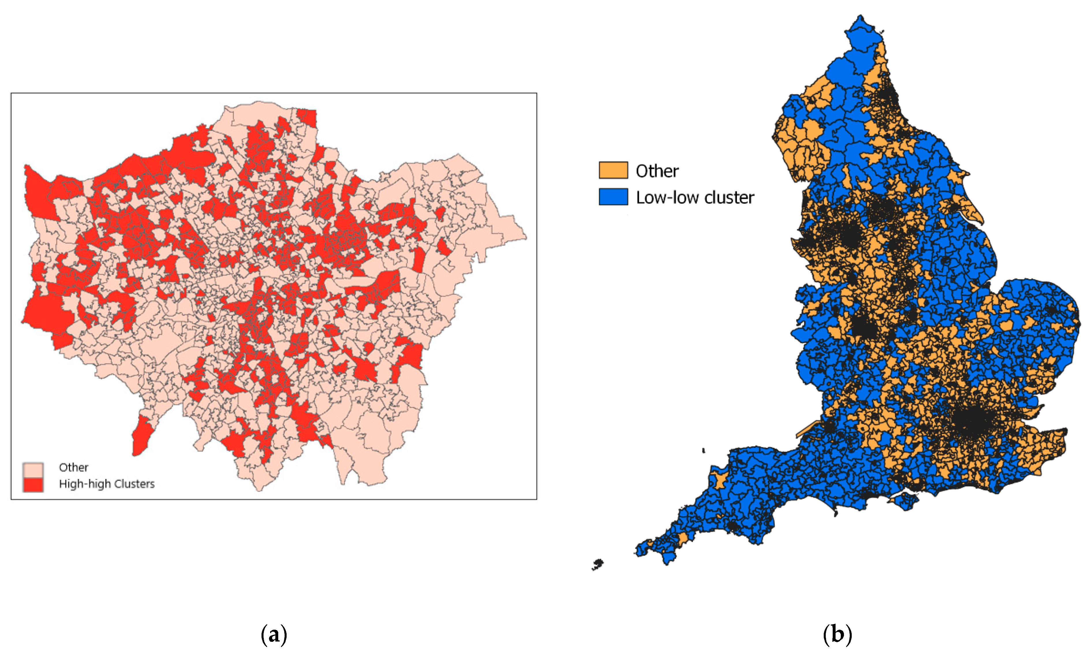
Within metropolitan regions, the extent of clustering is variable according to such characteristics. For example, in London boroughs with large ethnic populations, and often high deprivation, (e.g., Brent, Newham, Harrow), most neighborhoods are high-mortality clusters (see Figure 1a), whereas affluent suburban boroughs (Richmond, Havering), with relatively small BAME communities, have under 10% of neighborhoods constituting high-risk clusters.
There are 1367 low-mortality cluster centers, concentrated in more rural settings and smaller towns. Sixty-two percent of MSOAs in the two most rural categories (“rural and dispersed”) are low-mortality cluster centers. Figure 1b shows the location of low-mortality clusters, mainly in rural areas across England.
The metropolitan–rural contrast in mortality clustering is paramount but there are also regional contrasts. Thus 68% of MSOAs in South West England are classed as low-risk clusters. Even in more urban settings in the South West (such as “Urban City & Town”), the South West is under-represented in the proportion of high-mortality clusters.
5. Discussion
Reviews of differential COVID mortality (e.g., [2]) mention both individual demographic risk factors (e.g., ethnicity) and area contexts. There may be a gain in establishing contextual impacts to consider spatially contextual expressions of demographic risk factors [13].
Regarding area contexts, environmental factors have also been proposed, including debate regarding pollution’s influence on COVID-19 outcomes. An international study [35] found relatively large contributions to attributable mortality from air pollution. However, a UK review [30] was more skeptical, suggesting correlation between pollution and mortality was related to the epidemic’s original urban concentration, saying “correlation is smaller than measured or perhaps non-existent, and […] an early association between air pollution and COVID-19 mortality was linked to an initial outbreak of disease in large urban centres.” This review also found confounding between ethnicity and pollution, and between urbanicity and pollution, suggesting that high pollution levels are “proxies for increasingly urban areas”.
Analysis of mortality gradients in this study (see Table 2) shows significant increasing gradients for all sociodemographic indices, and for overall measures of the two environmental factors considered. Of note are relatively steep gradients associated with ethnicity and particular pollutants, especially NO2 [73,74,75]. However, this analysis does not control for multicollinearity or allow for mediated effects.
The regression analysis shows significant impacts of socio-demographic factors, namely health deprivation and ethnic mix, on COVID mortality. Slightly better predictions are obtained using a BAME segregation measure rather than simple BAME proportions. This may represent impacts of spatial variations in housing and labor market opportunities, which affect BAME residential location, and can be considered more specifically contextual measures [13].
Impacts of population mix and ethnic segregation are important in terms of a “sustainable COVID-19 public health strategy” [76]. Arguably, such a strategy should allow for different local risks to impact future epidemic containment plans, prioritizing higher risk areas in terms of mitigation measures and resources.
However, after accounting for socio-demographic factors, there are strong associations between air quality and COVID mortality, which demonstrates an impact of a purely contextual risk factor. Under the better fitting model, there is a virtually two-fold (1.74) relative mortality risk between neighborhoods with poor air quality as against those with good air quality. This finding regarding the impact of pollution is obtained despite mortality data covering a five month period, namely the full extent of the UK epidemic’s first wave, during which there was some diffusion in epidemic mortality from urban centers. Similar UK specific findings have been reported elsewhere but at a spatially aggregated rather than neighborhood scale [77].
This result highlights the policy importance of longer term environmental measures in addition to epidemic mitigation. It suggests that if pollution in certain neighborhoods remains high, then COVID mortality in these areas in any future epidemic is likely to also be elevated.
Further research is needed on issues such as which pollutants are most implicated. As a US study [3] mentions, “Although we found a strong positive association between air pollution and the risk of COVID-19-related death, the role of long-term exposure to poor air quality on COVID-19-related deaths […] is still not well understood”.
The regression shows some unexpected findings. Thus, the deprivation effect is more clearly related to health than material factors. In both regressions (models 1 and 2), the HDD domain shows a strong positive impact in raising mortality, while there is only a small positive effect of income deprivation. Table 6 shows a steep gradient in health deprivation as income deprivation increases, and a mediating effect of health deprivation in the impact of area income levels is plausible. This is confirmed using reduced regressions (see Section 4.2). The effect of income deprivation is almost nullified when area morbidity is also a predictor, whereas its impact is considerable when area morbidity is excluded from the regression—suggesting its effect is almost entirely mediated.
As [4] states, with regard to male COVID mortality, “people in disadvantaged groups, and men in particular, have higher rates of almost all of the known underlying clinical risk factors that increase the severity and mortality of COVID-19”. The policy relevance of the morbidity–SES nexus is discussed in [78].
The regression analysis also shows that the impact of ethnicity in increasing mortality is partly mediated by poor air quality: The impact of ethnicity is much increased when air quality is excluded as a predictor. In other words, air quality is a contextual mediator. This reflects differential ethnic exposures to poor air quality. For example, Table 6 shows that poor air quality is more strongly associated with ethnic mix than with income deprivation (a proxy for area socio-economic status).
Similar themes are raised by US research, such as [79,80]. Thus, [80] mentions “racial disparities in exposure to environmental pollutants are greater factors [influencing COVID outcomes] that remain even after controlling for income”. In the UK, a previous study [81] mentions pollution as an intervening variable in impacts of ethnicity on adverse COVID outcomes, while a review of COVID risk factors by Public Health England (PHE) has been criticized for omitting pollution. The commentary [82] mentions that “the [PHE] review therefore wrongly projects the idea that [minority ethnic] communities may be more susceptible to coronavirus, when it should instead say they are put into harm’s way by living in more polluted areas.”
In both the US and UK, ethnic minorities are more concentrated than the rest of the population in highly urbanized environments where air pollution is worse. The study [30] notes the strong association between ethnic concentration and air quality.
The greenspace effect also appears to be mediated by air quality. The environmental pathways that might explain this have been explored in other studies [83]. Again, air quality is acting as a contextual mediator in explaining variation in COVID-19 mortality.
The main feature from analyzing mortality high-risk clustering is a pronounced metropolitan–rural contrast, rather than (say) a North–South contrast. By contrast, all-cause mortality in England, albeit in years preceding the COVID epidemic, evinces a North–South divide [84]. The regression analysis suggests that concentration of high-risk clusters in the most metropolitan category reflects higher health deprivation, BAME concentration/segregation, and worse air quality.
Certain limitations to the work here may be mentioned. The analysis here concerns the UK COVID-19 first wave. Any conclusions may not extend to later epidemic waves or other nations—though there is evidence that some risk factor patterns, such as ethnicity-related risk, have continuity between the waves [85]. The analysis also has to acknowledge that ecological studies cannot establish impacts of individual risk factors, merely how they are indirectly reflected in “compositional” effects [86]. However, neighborhood COVID-19 mortality data are able to provide a comprehensive population level perspective for one of the UK nations, one relevant to setting public health priorities [25].
6. Conclusions
The analysis here benefits from covering the full time extent of the first wave in England, by using a small area scale (average population under 10,000 in each area), and by using regression allowing for spatial aspects of risk, including unobserved spatially clustered influences.
The results support a multifactorial explanation of varying neighborhood COVID mortality, involving both environmental and sociodemographic influences, and both compositional and contextual factors. Leading variables associated with varying mortality are air quality, health deprivation, and ethnicity. This is apparent both from mortality gradients, and from regression analysis controlling for multicollinearity and unobserved spatially clustered risk factors. Translating regression results into implications for mortality clusters we find a metropolitan-rural contrast across English neighborhoods as paramount.
Funding
This research received no external funding.
Data Availability Statement
Data are from the ONS website for “Deaths involving COVID-19 by local area and socioeconomic deprivation: deaths occurring between 1 March and 31 July 2020”.
Conflicts of Interest
The authors declare no conflict of interest.
References
- Office of National Statistics. Deaths Involving COVID-19 by Local Area and Socioeconomic Deprivation: Deaths Occurring between 1 March 2020 and 31 July 2020; Statistical Bulletin, ONS: London, UK, 2020. Available online: https://www.ons.gov.uk/ (accessed on 5 December 2020).
- Public Health England. Disparities in the Risk and Outcomes of COVID-19; PHE: London, UK, 2020. [Google Scholar]
- Correa-Agudelo, E.; Mersha, T.; Branscum, A.; MacKinnon, N.; Cuadros, D. Identification of vulnerable populations and areas at higher risk of Covid-19-related mortality during the early stage of the epidemic in the United States. Int. J. Environ. Res. Public Health 2021, 18, 4021. [Google Scholar] [CrossRef]
- Baker, P. Men, deprivation and COVID-19. Trends Urol. Men’s Health 2021, 12, 22–25. [Google Scholar] [CrossRef]
- Public Health Scotland (PHS). What Explains the Spatial Variation in COVID-19 Mortality across Scotland? PHS: Edinburgh, Scotland, 2020. [Google Scholar]
- Rose, T.; Mason, K.; Pennington, A.; McHale, P.; Taylor-Robinson, D.; Barr, B. Inequalities in COVID19 mortality related to ethnicity and socioeconomic deprivation. MedRxiv 2020. Available online: https://www.medrxiv.org/content/10.1101/2020.04.25.20079491v2 (accessed on 10 April 2021).
- Quinio, V. Have UK Cities Been Hotbeds of the Covid-19 Pandemic? Centre for Cities. Available online: https://www.centreforcities.org/blog/have-uk-cities-been-hotbeds-of-covid-19-pandemic (accessed on 15 December 2020).
- Ali, N.; Islam, F. The effects of air pollution on Covid-19 infection and mortality—A review on recent evidence. Front. Public Health 2020, 8, 580057. [Google Scholar] [CrossRef]
- Diez Roux, A. Investigating neighborhood and area effects on health. Am. J. Public Health 2001, 91, 1783–1789. [Google Scholar] [CrossRef] [PubMed]
- Cordes, J.; Castro, M. Spatial analysis of COVID-19 clusters and contextual factors in New York City. Spat. Spatio-Temporal Epidemiol. 2020, 34, 100355. [Google Scholar] [CrossRef]
- Thompson Coon, J.; Boddy, K.; Stein, K.; Whear, R.; Barton, J.; Depledge, M. Does participating in physical activity in outdoor natural environments have a greater effect on physical and mental wellbeing than physical activity indoors? A systematic review. Environ. Sci. Technol. 2011, 45, 1761–1772. [Google Scholar] [CrossRef]
- Macintyre, S. Deprivation amplification revisited; or, is it always true that poorer places have poorer access to resources for healthy diets and physical activity? Int. J. Behav. Nutr. Phys. 2007, 4, 32. [Google Scholar] [CrossRef] [PubMed] [Green Version]
- White, K.; Borrell, L. Racial/ethnic residential segregation: Framing the context of health risk and health disparities. Health Place 2011, 17, 438–448. [Google Scholar] [CrossRef] [PubMed] [Green Version]
- Darlington-Pollock, F.; Norman, P. Examining ethnic inequalities in health and tenure in England: A repeated cross-sectional analysis. Health Place 2017, 46, 82–90. [Google Scholar] [CrossRef] [PubMed]
- Phillips, D. Black minority ethnic concentration, segregation and dispersal in Britain. Urban Stud. 1998, 35, 1681–1702. [Google Scholar] [CrossRef]
- Mitchell, G.; Dorling, D. An environmental justice analysis of British air quality. Environ. Plan. A 2003, 35, 909–929. [Google Scholar] [CrossRef] [Green Version]
- Mitchell, G. The Messy Challenge of Environmental Justice in the UK: Evolution, Status and Prospects; Natural England Commissioned Report NECR273; Natural England: London, UK, 2019. [Google Scholar]
- Liang, D.; Shi, L.; Zhao, J.; Liu, P.; Sarnat, J.; Gao, S.; Schwartz, J.; Liu, Y.; Ebelt, S.; Scovronick, N.; et al. Urban Air Pollution May Enhance COVID-19 Case-Fatality and Mortality Rates in the United States. Innovation 2020, 1, 100047. [Google Scholar] [CrossRef] [PubMed]
- Wu, X.; Nethery, R.; Sabath, M.; Braun, D.; Dominici, F. Air pollution and COVID-19 mortality in the United States: Strengths and limitations of an ecological regression analysis. Sci. Adv. 2020, 6, eabd4049. [Google Scholar] [CrossRef]
- Dobricic, S.; Pisoni, E.; Pozzoli, L.; Van Dingenen, R.; Lettieri, T.; Wilson, J.; Vignati, E. Do Environmental Factors such as Weather Conditions and Air Pollution Influence COVID-19 Outbreaks; EUR 30376 EN; Publications Office of the European Union: Luxembourg, 2020. [Google Scholar]
- Heederik, D.; Smit, L.; Vermeulen, R. Go slow to go fast: A plea for sustained scientific rigour in air pollution research during the COVID-19 pandemic. Eur. Respir. J. 2020, 56, 2001361. [Google Scholar] [CrossRef] [PubMed]
- Evans, G.; Kantrowitz, E. Socioeconomic status and health: The potential role of environmental risk exposure. Annu. Rev. Public Health 2002, 23, 303–331. [Google Scholar] [CrossRef] [PubMed] [Green Version]
- Erqou, S.; Clougherty, J.; Olafiranye, O.; Magnani, J.; Aiyer, A.; Tripathy, S.; Kinnee, E.; Kip, K.; Reis, S. Particulate matter air pollution and racial differences in cardiovascular disease risk. Arterioscler. Thromb. Vasc. Biol. 2018, 38, 935–942. [Google Scholar] [CrossRef] [PubMed] [Green Version]
- Babyak, M. Understanding confounding and mediation. Evid. Based Ment. Health 2009, 12, 68–71. [Google Scholar] [CrossRef] [PubMed]
- Pearce, N. The ecological fallacy strikes back. J. Epidemiol. Community Health 2000, 54, 326–327. [Google Scholar] [CrossRef] [Green Version]
- Pinzari, L.; Mazumdar, S.; Girosi, F. A framework for the identification and classification of homogeneous socioeconomic areas in the analysis of health care variation. Int. J. Health Geogr. 2018, 17, 42. [Google Scholar] [CrossRef]
- Kang, S.; Cramb, S.; White, N.; Ball, S.; Mengersen, K. Making the most of spatial information in health: A tutorial in Bayesian disease mapping for areal data. Geospat. Health 2016, 11, 190–198. [Google Scholar] [CrossRef] [Green Version]
- Bell, D.; Comas-Herrera, A.; Henderson, D.; Jones, S.; Lemmon, E.; Moro, M.; Murphy, S.; O’Reilly, D.; Patrignani, P. COVID-19 Mortality and Long-Term Care: A UK Comparison. International Long-Term Care Policy Network, CPEC-LSE. Available online: https://ltccovid.org/2020/08/28/covid-19-mortality-and-long-term-care-a-uk-comparison/ (accessed on 16 January 2021).
- Ssentongo, P.; Ssentongo, A.; Heilbrunn, E.; Ba, D.; Chinchilli, V. Association of cardiovascular disease and 10 other pre-existing comorbidities with COVID-19 mortality: A systematic review and meta-analysis. PLoS ONE 2020, 15, e0238215. [Google Scholar] [CrossRef] [PubMed]
- Dutton, A. Coronavirus (COVID-19) Related Mortality Rates and the Effects of Air Pollution in England; Office of National Statistics: London, UK, 2020. [Google Scholar]
- Aldridge, R.; Lewer, D.; Katikireddi, S.; Mathur, R.; Pathak, N.; Burns, R.; Fragaszy, E.; Johnson, A.; Devakumar, D.; Abubakar, I.; et al. Black, Asian and Minority Ethnic groups in England are at increased risk of death from COVID-19: Indirect standardisation of NHS mortality data. Wellcome Open Res. 2020, 5, 88. [Google Scholar] [CrossRef] [PubMed]
- Office for National Statistics. Which Occupations Have the Highest Potential Exposure to the Coronavirus (COVID-19)? ONS: London, UK, 2020. [Google Scholar]
- Sun, Y.; Hu, X.; Xie, J. Spatial inequalities of COVID-19 mortality rate in relation to socioeconomic and environmental factors across England. Sci. Total Environ. 2020, 13, 143595. [Google Scholar] [CrossRef]
- Baena-Díez, J.; Barroso, M.; Cordeiro-Coelho, S.I.; Díaz, J.; Grau, M. Impact of COVID-19 outbreak by income: Hitting hardest the most deprived. J. Public Health 2020, 42, 698–703. [Google Scholar] [CrossRef]
- Pozzer, A.; Dominici, F.; Haines, A.; Witt, C.; Münzel, T.; Lelieveld, J. Regional and global contributions of air pollution to risk of death from COVID-19. Cardiovasc. Res. 2020, 116, cvaa288. [Google Scholar] [CrossRef]
- Bray, I.; Gibson, A.; White, J. Coronavirus disease 2019 mortality: A multivariate ecological analysis in relation to ethnicity, population density, obesity, deprivation and pollution. Public Health 2020, 185, 261–263. [Google Scholar] [CrossRef]
- Matheson, J.; Nathan, M.; Pickard, H.; Vanino, E. Why Has Coronavirus Affected Cities More Than Rural Areas? Economics Observatory. Available online: https://www.coronavirusandtheeconomy.com (accessed on 10 February 2021).
- Rojas-Rueda, D.; Nieuwenhuijsen, M.; Gascon, M.; Perez-Leon, D.; Mudu, P. Green spaces and mortality: A systematic review and meta-analysis of cohort studies. Lancet Planet. Health 2019, 3, e469–e477. [Google Scholar] [CrossRef] [Green Version]
- Gladwell, V.; Brown, D.; Wood, C.; Sandercock, G.; Barton, J. The great outdoors: How a green exercise environment can benefit all. Extrem. Physiol. Med. 2013, 2, 1–7. [Google Scholar] [CrossRef] [Green Version]
- American Association for the Advancement of Science (AAAS). COVID-19: Exercise May Protect against Deadly Complication, 15-04-2020. Available online: https://www.eurekalert.org/pub_releases/2020-04/uovh-cem041520.php (accessed on 12 December 2020).
- Ferguson, M.; Roberts, H.; McEachan, R.; Dallimer, M. Contrasting distributions of urban green infrastructure across social and ethno-racial groups. Landsc. Urban Plan. 2018, 175, 136–148. [Google Scholar] [CrossRef]
- Harris, R. Exploring the neighborhood-level correlates of Covid-19 deaths in London using a difference across spatial boundaries method. Health Place 2020, 66, 102446. [Google Scholar] [CrossRef] [PubMed]
- Kulu, H.; Dorey, P. Infection rates from COVID-19 in Great Britain by geographical units: A model-based estimation from mortality data. Health Place 2020, 66, 102460. [Google Scholar] [CrossRef] [PubMed]
- Sun, F.; Matthews, S.; Yang, T.; Hu, M. A spatial analysis of the COVID-19 period prevalence in US counties through June 28, 2020: Where geography matters? Ann. Epidemiol. 2020. epub ahead of print. [Google Scholar] [CrossRef]
- Huang, G.; Brown, P. Population-weighted exposure to air pollution and COVID-19 incidence in Germany. Spat. Stat. 2021, 41, 100480. [Google Scholar] [CrossRef] [PubMed]
- Hoeting, J. The importance of accounting for spatial and temporal correlation in analyses of ecological data. Ecol. Appl. 2009, 19, 574–577. [Google Scholar] [CrossRef] [PubMed]
- Beale, C.; Lennon, J.; Yearsley, J.; Brewer, M.; Elston, D. Regression analysis of spatial data. Ecol. Lett. 2010, 13, 246–264. [Google Scholar] [CrossRef] [PubMed]
- Cuzick, J. A Wilcoxon-type test for trend. Stat. Med. 1985, 4, 87–89. [Google Scholar] [CrossRef] [PubMed]
- Lawson, A.; Lee, D. Bayesian Disease Mapping for Public Health; Chapter 16 in Handbook of Statistics; Elsevier: Amsterdam, The Netherlands, 2017; Volume 36, pp. 443–481. [Google Scholar]
- Waller, L.; Carlin, B. Disease mapping. In Chapter 14 in Chapman Hall/CRC Handbook of Modern Statistical Methods; CRC: Boca Raton, FL, USA, 2010; pp. 217–243. [Google Scholar]
- Leroux, B.; Lei, X.; Breslow, N. Estimation of disease rates in small areas: A new mixed model for spatial dependence. In Statistical Models in Epidemiology, the Environment and Clinical Trials; Halloran, M., Berry, D., Eds.; Springer: New York, NY, USA, 1999; pp. 135–178. [Google Scholar]
- Richardson, S.; Thomson, A.; Best, N.; Elliott, P. Interpreting posterior relative risk estimates in disease-mapping studies. Environ. Health Perspect. 2004, 112, 1016–1025. [Google Scholar] [CrossRef]
- Office of National Statistics (ONS). Deaths Involving COVID-19 by Local Area and Socioeconomic Deprivation: Deaths Occurring between 1 March and 31 July 2020; Statistical Bulletin, ONS: London, UK, 2020. [Google Scholar]
- Ministry of Housing, Communities and Local Government (MHCLG). English Indices of Deprivation 2019; MHCLG: London, UK, 2019. [Google Scholar]
- Ministry of Housing, Communities and Local Government (MHCLG). English Indices of Deprivation 2019; Technical Report; MHCLG: London, UK, 2019. [Google Scholar]
- Lieberson, S. An Asymmetrical Approach to Segregation. In Ethnic Segregation in Cities; Peach, C., Robinson, V., Smith, S., Eds.; Croom Helm: London, UK, 1981; pp. 61–82. [Google Scholar]
- Green, M.; Daras, K.; Davies, A.; Barr, B.; Singleton, A. Developing an openly accessible multi-dimensional small area index of ‘Access to Healthy Assets and Hazards’ for Great Britain. Health Place 2018, 54, 11–19. [Google Scholar] [CrossRef]
- Brookes, D.; Stedman, J.; Kent, A.; Whiting, S.; Rose, R.; Williams, C.; Pugsley, K. UK Supplementary Assessment under the Air Quality Directive (2008/50/EC), the Air Quality Framework Directive (96/62/EC) and Fourth Daughter Directive (2004/107/EC) for 2018; Technical Report; DEFRA: London, UK, 2020. Available online: https://uk-air.defra.gov.uk/library/reports?report_id=993 (accessed on 7 May 2021).
- Trust for London. Access to Healthy Assets and Hazards Index (Rebased for London) (2019). Available online: https://www.trustforlondon.org.uk/data/access-healthy-assets-and-hazards/ (accessed on 6 May 2021).
- Daras, K.; Green, M.; Davies, A.; Barr, B.; Singleton, A. Open data on health-related neighborhood features in Great Britain. Nat. Sci. Data 2019, 6, 107. [Google Scholar] [CrossRef]
- Office of National Statistics. Access to Gardens and Public Green Space in Great Britain. Available online: https://www.ons.gov.uk/economy/environmentalaccounts/datasets/accesstogardensandpublicgreenspaceingreatbritain (accessed on 6 May 2021).
- When and Why to Standardize Your Data? Available online: https://builtin.com/data-science/when-and-why-standardize-your-data (accessed on 3 May 2021).
- Available online: https://www.listendata.com/2017/04/how-to-standardize-variable-in-regression.html (accessed on 3 May 2021).
- Reich, B.; Fuentes, M.; Dunson, D. Bayesian spatial quantile regression. J. Am. Stat. Assoc. 2011, 106, 6–20. [Google Scholar] [CrossRef] [Green Version]
- Lunn, D.; Spiegelhalter, D.; Thomas, A.; Best, N. The BUGS project: Evolution, critique and future directions. Stat. Med. 2009, 28, 3049–3067. [Google Scholar] [CrossRef]
- Brooks, S.; Gelman, A. General methods for monitoring convergence of iterative simulations. J. Comput. Graph. Stat. 1998, 7, 434–455. [Google Scholar]
- Spiegelhalter, D.; Best, N.; Carlin, B.; van der Linde, A. Bayesian measures of model complexity and fit. J. R. Stat. Soc. Ser. B 2002, 64, 583–639. [Google Scholar]
- Lunn, D.; Jackson, C.; Best, N.; Thomas, A.; Spiegelhalter, D. The BUGS book. In A Practical Introduction to Bayesian Analysis; Chapman Hall: London, UK, 2013. [Google Scholar]
- Watanabe, S. Asymptotic Equivalence of Bayes Cross Validation and Widely Applicable Information Criterion in Singular Learning Theory. J. Mach. Learn. Res. 2010, 11, 3571–3594. [Google Scholar]
- Anselin, L.; Syabri, I.; Kho, Y. GeoDa: An introduction to spatial data analysis. Geogr. Anal. 2006, 38, 5–22. [Google Scholar] [CrossRef]
- Moraga, P.; Montes, F. Detection of spatial disease clusters with LISA functions. Stat. Med. 2011, 30, 1057–1071. [Google Scholar] [CrossRef] [PubMed]
- Bibby, P.; Brindley, P. The 2011 Rural-Urban Classification for Small Area Geographies: A User Guide and Frequently Asked Questions; Office for National Statistics: London, UK, 2013. [Google Scholar]
- Ogen, Y. Assessing nitrogen dioxide (NO2) levels as a contributing factor to coronavirus (COVID-19) fatality. Sci. Total Environ. 2020, 726, 138605. [Google Scholar] [CrossRef] [PubMed]
- Copat, C.; Cristaldi, A.; Fiore, M.; Grasso, A.; Zuccarello, P.; Santo Signorelli, S.; Conti, G.O.; Ferrante, M. The role of air pollution (PM and NO2) in COVID-19 spread and lethality: A systematic review. Environ. Res. 2020, 191, 110129. [Google Scholar] [CrossRef]
- Mele, M.; Magazzino, C.; Schneider, N.; Strezov, V. NO2 levels as a contributing factor to COVID-19 deaths: The first empirical estimate of threshold values. Environ. Res. 2021, 194, 110663. [Google Scholar] [CrossRef]
- Gurdasani, D.; Bear, L.; Bogaert, D.; Burgess, R.A.; Busse, R.; Cacciola, R.; Charpak, Y.; Colbourn, T.; Drury, J.; Friston, K.; et al. The UK needs a sustainable strategy for COVID-19. Lancet 2020, 396, 1800–1801. [Google Scholar] [CrossRef]
- Travaglio, M.; Yu, Y.; Popovic, R.; Selley, L.; Leal, N.; Martins, L. Links between air pollution and COVID-19 in England. Environ. Pollut. 2021, 268, 115859. [Google Scholar] [CrossRef]
- Anderson, G.; Frank, J.; Naylor, C.D.; Wodchis, W.; Feng, P. Using socioeconomics to counter health disparities arising from the covid-19 pandemic. Br. Med. J. 2020, 369, m2149. [Google Scholar] [CrossRef] [PubMed]
- Brandt, E.; Beck, A.; Mersha, T. Air pollution, racial disparities, and COVID-19 mortality. J. Allergy Clin. Immunol. 2020, 146, 61–63. [Google Scholar] [CrossRef]
- Washington, H. How environmental racism is fuelling the coronavirus pandemic. Nature 2020, 581, 241. [Google Scholar] [CrossRef] [PubMed]
- Soltan, M.; Crowley, L.; Melville, C.; Varney, J.; Cassidy, S.; Mahida, R.; Grudzinska, F.; Parekh, D.; Dosanjh, D.; Thickett, D. To what extent are social determinants of health, including household overcrowding, air pollution and housing quality deprivation, modulators of presentation, ITU admission and outcomes among patients with SARS-COV-2 infection in an urban catchment area in Birmingham, United Kingdom? Thorax 2021, 76, A237–A238. [Google Scholar]
- Carrington, D. Omission of Air Pollution from Report on Covid-19 and Race ‘Astonishing’; The Guardian: London, UK, 2020. [Google Scholar]
- Shen, Y.; Lung, S. Mediation pathways and effects of green structures on respiratory mortality via reducing air pollution. Sci. Rep. 2017, 7, 1–9. [Google Scholar] [CrossRef] [Green Version]
- Buchan, I.; Kontopantelis, E.; Sperrin, M.; Chandola, T.; Doran, T. North-South disparities in English mortality 1965–2015: Longitudinal population study. J. Epidemiol. Community Health 2017, 71, 928–936. [Google Scholar] [CrossRef] [PubMed] [Green Version]
- Mathur, R.; Rentsch, C.; Morton, C.; Hulme, W.; Schultze, A.; MacKenna, B.; Eggo, R.; Bhaskaran, K.; Wong, A.; Williamson, E.; et al. Ethnic differences in SARS-CoV-2 infection and COVID-19-related hospitalisation, intensive care unit admission, and death in 17 million adults in England: An observational cohort study using the OpenSAFELY platform. Lancet 2021, 397, 1711–1724. [Google Scholar] [CrossRef]
- Duncan, C.; Jones, K.; Moon, G. Context, composition and heterogeneity: Using multilevel models in health research. Soc. Sci. Med. 1998, 46, 97–117. [Google Scholar] [CrossRef]
Figure 1.
(a) High-mortality clusters in Londonl; (b) Low-mortality clusters across England.


Table 1.
Distributional Characteristics of Area Risk Variables.
| Risk Variable | Mean | Median | 95th Percentile | 5th Percentile | Maximum | Minimum | InterQuartile Range |
|---|---|---|---|---|---|---|---|
| Income Deprivation | 0.128 | 0.106 | 0.289 | 0.04 | 0.490 | 0.010 | 0.103 |
| Health Deprivation and Disability | −0.008 | −0.0306 | 1.268 | −1.22 | 2.868 | −3.045 | 1.084 |
| BAME, % in MSOA population | 13.7 | 5.3 | 56.8 | 1.2 | 94.4 | 0.4 | 14.6 |
| BAME Isolation Index | 0.148 | 0.061 | 0.584 | 0.014 | 0.946 | 0.005 | 0.160 |
| Nursing Home Location, % | 3.49 | 2.70 | 9.61 | 0.00 | 41.07 | 0.00 | 3.47 |
| Active Green Space Index (CDRC) | 0.60 | 0.50 | 1.28 | 0.27 | 6.91 | 0.10 | 0.28 |
| % Private Outdoor Space | 89 | 92 | 98 | 72 | 100 | 2 | 8 |
| Overall Greenspace Access | 0.0 | −0.1 | 1.7 | −1.4 | 6.7 | −11.8 | 0.8 |
| NO2 | 12.6 | 12.0 | 21.5 | 6.1 | 28.5 | 3.3 | 4.8 |
| PM10 | 13.5 | 13.8 | 16.8 | 10.1 | 17.5 | 7.6 | 3.7 |
| SO2 | 1.22 | 1.2 | 1.8 | 0.8 | 2.7 | 0.4 | 0.4 |
| Overall Air Quality (Higher for Worse) | 26.1 | 20.5 | 67.9 | 4.5 | 99.7 | 0.4 | 24.3 |
Table 2.
Gradients in COVID-19 Mortality (SMRs, March–July 2020) over English Neighbourhoods.
| Socio-Demographic | |||||||
| Income Deprivation | Health Deprivation and Disability | BAME, % in MSOA Population | BAME Isolation Index | Nursing Home Location | |||
| Decile 1 | 0.60 | 0.81 | 0.65 | 0.66 | 0.87 | ||
| Decile 2 | 0.76 | 0.83 | 0.72 | 0.74 | 0.88 | ||
| Decile 3 | 0.84 | 0.83 | 0.79 | 0.80 | 0.94 | ||
| Decile 4 | 0.83 | 0.88 | 0.92 | 0.89 | 0.93 | ||
| Decile 5 | 0.90 | 0.90 | 0.88 | 0.90 | 0.94 | ||
| Decile 6 | 1.03 | 0.99 | 0.99 | 0.97 | 0.91 | ||
| Decile 7 | 1.18 | 1.04 | 1.11 | 1.09 | 1.09 | ||
| Decile 8 | 1.28 | 1.14 | 1.19 | 1.21 | 1.04 | ||
| Decile 9 | 1.42 | 1.33 | 1.41 | 1.40 | 1.14 | ||
| Decile 10 | 1.71 | 1.51 | 2.02 | 2.02 | 1.23 | ||
| All Neighborhoods | 1.00 | 1.00 | 1.00 | 1.00 | 1.00 | ||
| Environmental | |||||||
| Active Green Space Access * | % Private Outdoor Space * | Overall Greenspace Access * | NO2 | PM10 | SO2 | Overall Air Quality (Higher for Worse) | |
| Decile 1 | 0.64 | 0.96 | 0.67 | 0.55 | 0.97 | 0.55 | 0.60 |
| Decile 2 | 0.84 | 0.96 | 0.83 | 0.74 | 1.08 | 0.76 | 0.76 |
| Decile 3 | 0.94 | 0.98 | 0.87 | 0.74 | 1.00 | 0.83 | 0.84 |
| Decile 4 | 0.97 | 0.94 | 0.97 | 0.93 | 0.75 | 0.91 | 0.83 |
| Decile 5 | 0.98 | 0.91 | 0.96 | 0.97 | 0.92 | 1.02 | 0.90 |
| Decile 6 | 1.08 | 0.92 | 1.08 | 1.04 | 0.97 | 1.09 | 1.03 |
| Decile 7 | 1.13 | 0.89 | 1.10 | 1.20 | 0.84 | 1.24 | 1.18 |
| Decile 8 | 1.15 | 1.01 | 1.13 | 1.26 | 0.90 | 1.32 | 1.28 |
| Decile 9 | 1.18 | 1.13 | 1.22 | 1.47 | 1.17 | 1.27 | 1.42 |
| Decile 10 | 1.37 | 1.41 | 1.43 | 1.70 | 1.67 | 1.41 | 1.70 |
| All Neighborhoods | 1.00 | 1.00 | 1.00 | 1.00 | 1.00 | 1.00 | 1.00 |
* Higher deciles for worse access and lower % private outdoor space.
Table 3.
Regression Coefficients, Associated Relative Risks and Fit. Two Models Compared.
| Model 1 | Model 2 | |||
|---|---|---|---|---|
| Regression Coefficient 1 | Implied Relative Risk 2,3 | Regression Coefficient 1 | Implied Relative Risk 2,3 | |
| Income Deprivation (ID) | 0.153 | 1.085 | 0.140 | 1.077 |
| BAME | 0.856 | 1.616 | ||
| BAME Isolation | 0.828 | 1.604 | ||
| Nursing Homes | 1.143 | 1.301 | 1.142 | 1.301 |
| Health Deprivation (HDD Domain) | 1.150 | 1.625 | 1.164 | 1.635 |
| Poor Green Space Access | 0.134 | 1.119 | 0.075 | 1.072 |
| Poor Air Quality | 0.841 | 1.714 | 0.860 | 1.735 |
| Fit Measures | ||||
| DIC | 38139 | 37945 | ||
| WAIC | 38140 | 37950 | ||
1 Significant coefficients (with 95% intervals confined to positive values) in bold. 2 Significant relative risks (with 95% intervals confined to values over 1) in bold. 3 Relative risks compare mortality at 95th and 5th percentile of risk factor scores.
Table 4.
COVID Mortality Clusters by Area Type.
| Numbers of MSOAs by Region and Urban Level | |||||||||
| Region | Rural & Dispersed (Sparse Setting) | Rural & Dispersed | Rural Town/Fringe (Sparse Setting) | Rural Town & Fringe | Urban City & Town (Sparse Setting) | Urban City & Town | Urban Minor Conurbation | Urban Major Conurbation | Total |
| East Midlands | 2 | 66 | 1 | 78 | 2 | 318 | 102 | 4 | 573 |
| East of England | 2 | 104 | 5 | 113 | 433 | 79 | 736 | ||
| London | 1 | 2 | 980 | 983 | |||||
| North East | 7 | 5 | 2 | 43 | 2 | 131 | 150 | 340 | |
| North West | 6 | 35 | 4 | 47 | 2 | 313 | 517 | 924 | |
| South East | 108 | 116 | 785 | 99 | 1108 | ||||
| South West | 14 | 125 | 5 | 81 | 4 | 471 | 700 | ||
| West Midlands | 7 | 58 | 41 | 1 | 290 | 338 | 735 | ||
| Yorkshire/Humber | 7 | 38 | 3 | 68 | 2 | 195 | 147 | 232 | 692 |
| Total | 45 | 539 | 20 | 588 | 13 | 2938 | 249 | 2399 | 6791 |
| High Mortality Clusters by Region and Urban Level | |||||||||
| Region | Rural/Dispersed (Sparse Setting) | Rural & Dispersed | Rural Town/Fringe (Sparse Setting) | Rural Town & Fringe | Urban City & Town (Sparse Setting) | Urban City & Town | Urban Minor Conurbation | Urban Major Conurbation | Total |
| East Midlands | 0 | 0 | 0 | 0 | 0 | 25 | 5 | 0 | 30 |
| East of England | 0 | 1 | 0 | 1 | 20 | 17 | 39 | ||
| London | 1 | 0 | 362 | 363 | |||||
| North East | 0 | 0 | 0 | 1 | 0 | 23 | 18 | 42 | |
| North West | 0 | 1 | 0 | 1 | 0 | 14 | 146 | 162 | |
| South East | 0 | 0 | 18 | 4 | 22 | ||||
| South West | 0 | 0 | 0 | 0 | 0 | 4 | 4 | ||
| West Midlands | 0 | 0 | 0 | 0 | 12 | 88 | 100 | ||
| Yorkshire/Humber | 0 | 0 | 0 | 0 | 0 | 7 | 14 | 41 | 62 |
| Total | 0 | 2 | 0 | 4 | 0 | 123 | 19 | 676 | 824 |
| Low mortality clusters by Region and Urban Level | |||||||||
| Region | Rural/Dispersed (Sparse Setting) | Rural & Dispersed | Rural Town/Fringe (Sparse Setting) | Rural Town & Fringe | Urban City & Town (Sparse Setting) | Urban City & Town | Urban Minor Conurbation | Urban Major Conurbation | Total |
| East Midlands | 2 | 43 | 1 | 23 | 1 | 59 | 5 | 0 | 134 |
| East of England | 2 | 66 | 5 | 49 | 101 | 1 | 224 | ||
| London | 0 | 0 | 6 | 6 | |||||
| North East | 6 | 3 | 1 | 2 | 2 | 6 | 9 | 29 | |
| North West | 5 | 9 | 1 | 10 | 1 | 18 | 0 | 44 | |
| South East | 43 | 50 | 160 | 3 | 256 | ||||
| South West | 13 | 104 | 5 | 69 | 4 | 280 | 475 | ||
| West Midlands | 7 | 30 | 13 | 1 | 31 | 1 | 83 | ||
| Yorkshire/Humber | 6 | 23 | 1 | 27 | 2 | 36 | 7 | 14 | 116 |
| Total | 41 | 321 | 14 | 243 | 11 | 691 | 12 | 34 | 1367 |
Table 5.
Risk Factor Profiles by Urban Type.
| HDD Score | Air Pollution | % BAME | BAME Isolation Index | |
|---|---|---|---|---|
| Rural & Dispersed (Sparse Setting) | 0.42 | 2.7 | 1.2 | 0.014 |
| Rural & Dispersed | 0.38 | 10.3 | 2.2 | 0.030 |
| Rural Town & Fringe (Sparse Setting) | 0.47 | 4.5 | 1.8 | 0.022 |
| Rural Town & Fringe | 0.43 | 13.2 | 2.8 | 0.034 |
| Urban City & Town (Sparse Setting) | 0.53 | 4.0 | 1.6 | 0.018 |
| Urban City & Town | 0.49 | 18.8 | 8.6 | 0.096 |
| Urban Minor Conurbation | 0.56 | 29.9 | 11.4 | 0.124 |
| Urban Major Conurbation | 0.52 | 42.1 | 25.8 | 0.272 |
Table 6.
Gradients in Health Deprivation (HDD) and Air Quality by Neighborhood Income Deprivation and % BAME.
Table 6.
Gradients in Health Deprivation (HDD) and Air Quality by Neighborhood Income Deprivation and % BAME.
| Neighbourhoods by Income Deprivation Decile | Average HDD | Neighbourhoods by % BAME Decile | Average HDD |
| 1 | −0.99 | 1 | −0.05 |
| 2 | −0.72 | 2 | −0.01 |
| 3 | −0.52 | 3 | 0.00 |
| 4 | −0.31 | 4 | −0.07 |
| 5 | −0.14 | 5 | −0.06 |
| 6 | 0.00 | 6 | −0.05 |
| 7 | 0.23 | 7 | −0.08 |
| 8 | 0.46 | 8 | 0.00 |
| 9 | 0.71 | 9 | 0.06 |
| 10 | 1.20 | 10 | 0.19 |
| All Neighborhoods | −0.01 | All Neighborhoods | −0.01 |
| Neighbourhoods by Income Deprivation Decile | Average Air Quality (Higher Scores for Worse Air Quality) | Neighbourhoods by % BAME Decile | Average Air Quality (Higher Scores for Worse Air Quality) |
| 1 | 20.7 | 1 | 9.8 |
| 2 | 19.0 | 2 | 13.3 |
| 3 | 20.2 | 3 | 16.0 |
| 4 | 21.6 | 4 | 17.1 |
| 5 | 22.6 | 5 | 19.3 |
| 6 | 27.1 | 6 | 22.6 |
| 7 | 30.0 | 7 | 27.2 |
| 8 | 33.5 | 8 | 33.3 |
| 9 | 34.0 | 9 | 46.5 |
| 10 | 32.4 | 10 | 55.8 |
| All Neighborhoods | 26.1 | All Neighborhoods | 26.1 |
Publisher’s Note: MDPI stays neutral with regard to jurisdictional claims in published maps and institutional affiliations. |
© 2021 by the author. Licensee MDPI, Basel, Switzerland. This article is an open access article distributed under the terms and conditions of the Creative Commons Attribution (CC BY) license (https://creativecommons.org/licenses/by/4.0/).
Share and Cite
MDPI and ACS Style
Congdon, P. COVID-19 Mortality in English Neighborhoods: The Relative Role of Socioeconomic and Environmental Factors. J 2021, 4, 131-146. https://0-doi-org.brum.beds.ac.uk/10.3390/j4020011
AMA Style
Congdon P. COVID-19 Mortality in English Neighborhoods: The Relative Role of Socioeconomic and Environmental Factors. J. 2021; 4(2):131-146. https://0-doi-org.brum.beds.ac.uk/10.3390/j4020011
Chicago/Turabian StyleCongdon, Peter. 2021. "COVID-19 Mortality in English Neighborhoods: The Relative Role of Socioeconomic and Environmental Factors" J 4, no. 2: 131-146. https://0-doi-org.brum.beds.ac.uk/10.3390/j4020011