Automated Damage Detection of (C/C)/Si/SiC Composite Using Vibration Modes with Deep Neural Networks

Abstract

Discontinuous carbon fiber-carbon matrix composites dispersed Si/SiC matrix composites have complicated microstructures that consist of four phases (C/C, Si, SiC, and C/SiC). The crack stability significantly depends on their geometrical arrangement. Nondestructive evaluation is needed to maintain the components in their safe condition. Although several nondestructive evaluation methods such as the Eddy current have been developed, any set of them is still inadequate in order to cover all of the scales and aspects that (C/C)/Si/SiC composites comprise. We propose a new method for nondestructive evaluation using vibration/resonance modes and deep learning. The assumed resolution is mm-order (approx. 1–10 mm), which laser vibrometers are generally capable of handling sufficiently. We utilize deep neural networks called convolutional auto-encoders for inferring damaged areas from vibration modes, which is a so-called inverse problem and infeasible to solve numerically in most cases. We solve this inference problem by training convolutional auto-encoders using vibration modes obtained from a non-damaged specimen with various frequencies as the dataset. Experimental results show that the proposed method successfully detects the damaged areas of validation specimens. One of the noteworthy points of this method is that we need only a few specimens for training deep neural networks, which generally require a large amount of data.

1. Introduction

Discontinuous carbon fiber-carbon matrix (C/C) composites dispersed Si/SiC matrix composites (hereafter denoted as (C/C)/Si/SiC composites) have been expected for applications of light-weight structural components, such as car/motorbike brake disks [1,2], emergency brakes for elevators [3], and high-performance wear components, etc. Mechanical performances of (C/C)/Si/SiC composites have been extensively studied [4], and those reports have shown unique mechanical performances of the composites, which are difficult to obtain for monolithic ceramics and metals. In application, (C/C)/Si/SiC composites are subjected to various kinds of mechanical damage. Anomaly such as damage should be detected at maintenance periods, where it is decided whether the components are continuously used or replaced. Suitable nondestructive evaluation (NDE) is needed to maintain the components in their safe condition.

The characteristic properties of (C/C)/Si/SiC should be considered for NDE. It is known that (C/C)/Si/SiC composite exhibits extremely low fracture toughness under the assumption of linear elastic fracture mechanics [5]. In fact, the value is close to monolithic engineering ceramics [6]. Therefore, once a composite has a source of some stress concentration where tensile/shear loads are applied, then the composite falls into a dangerous situation as a component-bearing load because the fracture strength of the composite becomes ~$\frac{K_{Ic}}{\sqrt{a_{eff}}}$: $a_{eff}$ is the effective crack size [7]. 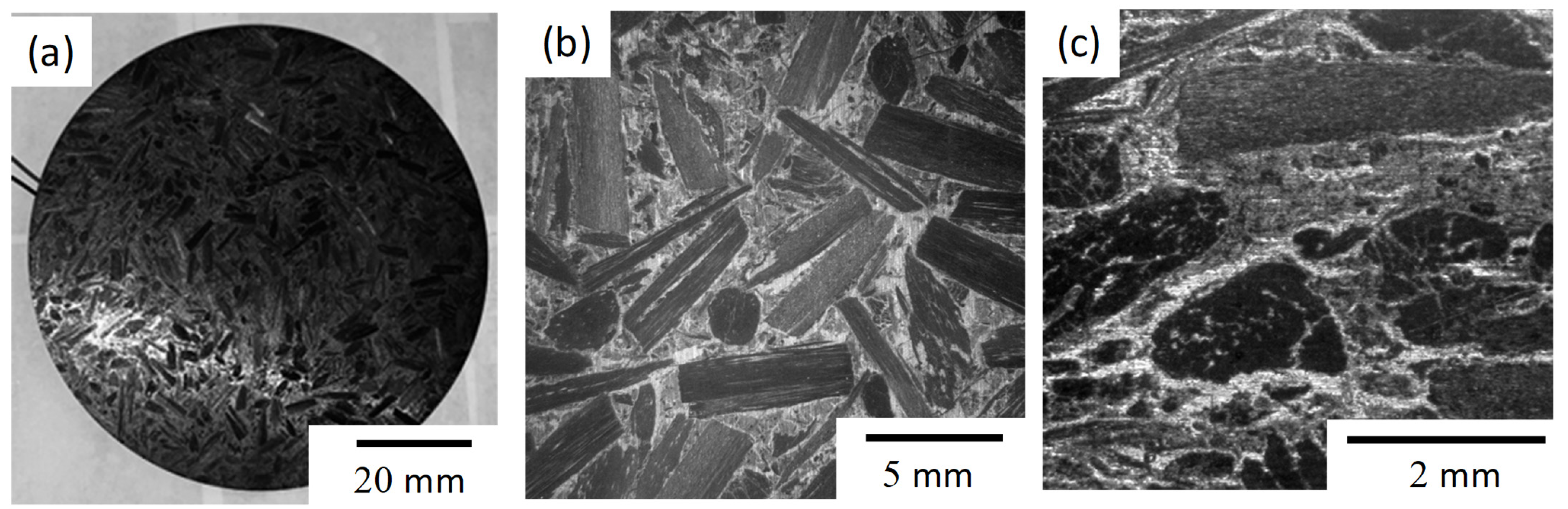Here, the effective crack size, $a_{eff}$, means the length scale for possible application of continuum mechanics (at least ten times larger than the microstructural units [7]). The microstructure of the composites is complicated: the structure consists of four major phases, C/C, Si, SiC, and C/SiC [8], and the crack stability in the composite is affected by the geometrical arrangement of these four major phases [8]. In addition, many microcracks are formed in the as-fabricated condition of the composites due to residual stress, which originates from thermal expansion mismatches and phase transformations of Si/SiC, etc. Dangerous mm-order damage zones including cracks close to $a_{eff}$ ~ mm order should be detected with a relatively simple process for safe operation.

Some nondestructive evaluation (NDE) methods have been applied for (C/C)/Si/SiC composite components. The Eddy current method could detect the progress of damage during service, and convenient test equipment has been commercially available [9]. Pulse-phase thermography could give inhomogeneous microstructure and is effective for a thin specimen [10]. When a component is thick or does not have a constant thickness, overwrapping different local thermal conductivity makes it difficult to analyze thermal imaging results. In addition, the technique is too sensitive concerning the environmental temperature and not easy to conduct, unlike other conventional tests. While each evaluation method has merits and demerits, no method is better in every way possible. Novel NDE methods for (C/C)/Si/SiC components still need to be developed.

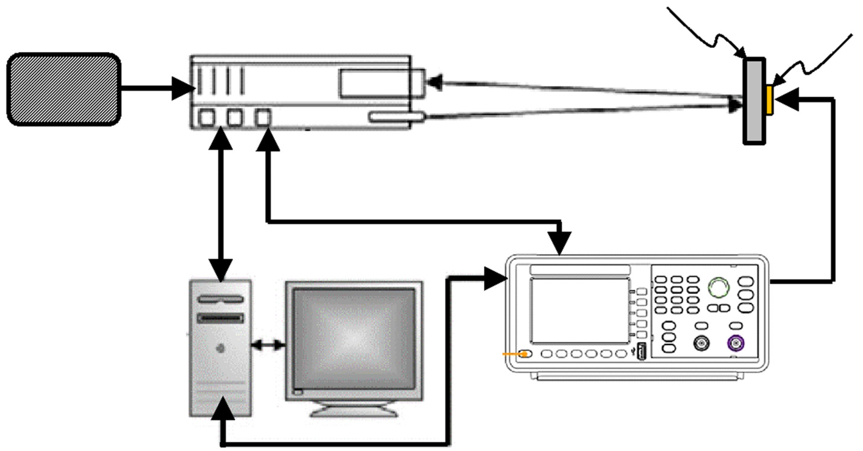
Recently, the authors applied simple vibration methods for (C/C)/Si/SiC composite [11]. The vibration-resonance frequency relation has been used for detection of nonuniformity, local damage, quality assessment of rotating components, etc. Laser holographic technique allows very sensitive detection of surface displacement images under forced vibration mode. Using the equipment and seeping vibration frequencies, it is possible to measure two-dimensional surface displacements of components with a nanometer-order displacement resolution. The method is highly reproducible and sensitive to the local density change of the target component.

Data processing/image analysis of the obtained vibration image allows for detection of local damage; however, the method only gives enhanced contrast of the detected images, and it is difficult to incorporate adequate threshold levels to ensure safe operation of the composite. Recently, AI is expected to use the criteria determination of available NDE methods [12]. However, the application of AI technologies usually needs a sufficient “database,” which is very hard to prepare. Therefore, the application of AI is still limited and remains at conceptual levels. Typically, in the field of (C/C)/Si/SiC the preparation of a database is very difficult because of limited data.

The present study has been focused on the application of “database free” AI technology for damage detection of (C/C)/Si/SiC composite. Discussions are made on the future application procedure of the present method. For safety applications, damage caused by mechanical impact should be clearly detected and classified as either “safe” or “dangerous” damage. Reports have shown that the impact damage of fiber-reinforced ceramic matrix composite strongly depends on the local damage accumulation behavior of the composites.

2. Macroscopic-Level Nondestructive Evaluation Using Vibration Modes

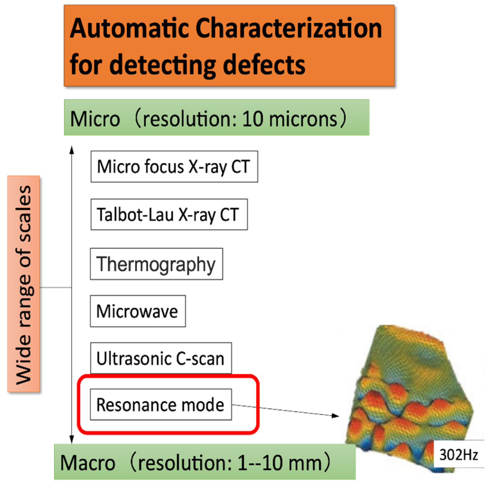
As mentioned in the introduction, yet another NDE method is required for evaluating disparate aspects that (C/C)/Si/SiCs have in various scales (Figure 1). The focus of this paper is the detection of macroscopic-level areas that deviate from the normal state with respect to some physical properties such as elasticity and strength. We assume that the resolution for the detection is mm-order (approx. 1–10 mm), which the measurement system of vibration and resonance modes is sufficiently capable of handling. The special resolution depends on some parameters, such as the elasticity and the vibration frequency. The laser vibrometer, which we used, observes the displacements in the Z-axis direction on the XY plane by irradiating the laser to the surface while the object is vibrated with a particular frequency.

We assume that sound pressure is uniform throughout the given space. In this scenario, the displacement map is uniquely determined by its sound frequency. Various patterns of the displacement maps are observed by changing the frequencies. In this paper, we call the observed displacement map for a frequency f a vibration mode for f. Several peaks are observed with respect to the squared means of the modes when the frequencies are changed. Since those peaks indicate resonance, the mode where a frequency generates a peak is called a resonance mode.

The physical properties, such as elastic modulus, locally change if the deviation occurs in some areas due to damage in the components. Those changes cause disturbances in the patterns of the vibration modes. If we recognize the irregular changes of the vibration pattern correctly, it is possible to detect the areas that have a shift of physical properties, which means damage of some kind in the component. However, solving this type of inverse problem is not feasible in most cases by numerical approaches such as finite element methods. So far, because we need to construct some physical property changes from the variations of the modes, no particular methods are yet known to solve them reliably in a systematic way. In addition, it is difficult to extract the precise frequencies that are useful for damage detection within the range specified. It is not realistic to examine manually what frequencies are most effective for specifying the damaged area. Automation is required from a practical perspective. The ideal conditions that our approach should satisfy are summarized as follows:

• For some frequencies, the irregular areas are extracted from the image of the vibration mode when the object is damaged. Irregular areas denote the areas deviating from regular wave patterns that non-damaged objects should have;
• For any frequencies, no areas are extracted when the object is non-damaged or has no significant deviations in terms of physical properties.

Note that the deviation of physical properties should be close to the surface where the vibration mode is measured because, generally speaking, the vibrometer measures the displacement only from a particular direction.

We need to define the regular wave patterns in (1). However, it is difficult to define them in an explicit way, such as numerical conditions on hand-made features. Instead, we utilize deep neural networks to learn the patterns that non-damaged objects normally have. Those patterns are learned from the data of the various modes, or the displacement images of many frequencies.

3. Methodology

3.1. Detection of Irregular Patterns on Vibration Modes with Auto-Encoders

The methods of anomaly detection, or outlier detection, are recently more successful in accurately detecting higher-level anomalies, because of the wide development of deep learning techniques [13,14]. Various kinds of data such as images, sounds, texts, and numerical features are considered as inputs for anomaly detection in general. Among them, it had been difficult to detect anomalies from rich data that contain abstract information, such as images, until deep learning emerged and was developed. Convolutional deep neural networks (CNNs) are one of the well-known neural architectures which are known to be superior for most image-related tasks such as image recognition and segmentation [15,16]. CNNs generally have multiple layers that transform input tensors and disentangle them sequentially so that the target task becomes solvable. The transformed vector/tensor embeddings of images are obtained by feeding the images into the layers of the trained CNNs. For instance, if a CNN is trained for some image classification tasks, the output vectors of the penultimate layer naturally distribute clusters into the task’s categories.

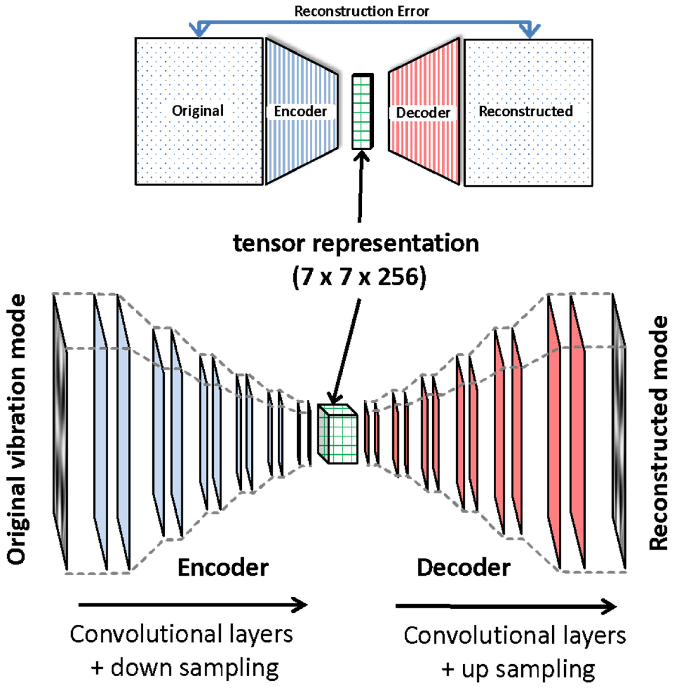
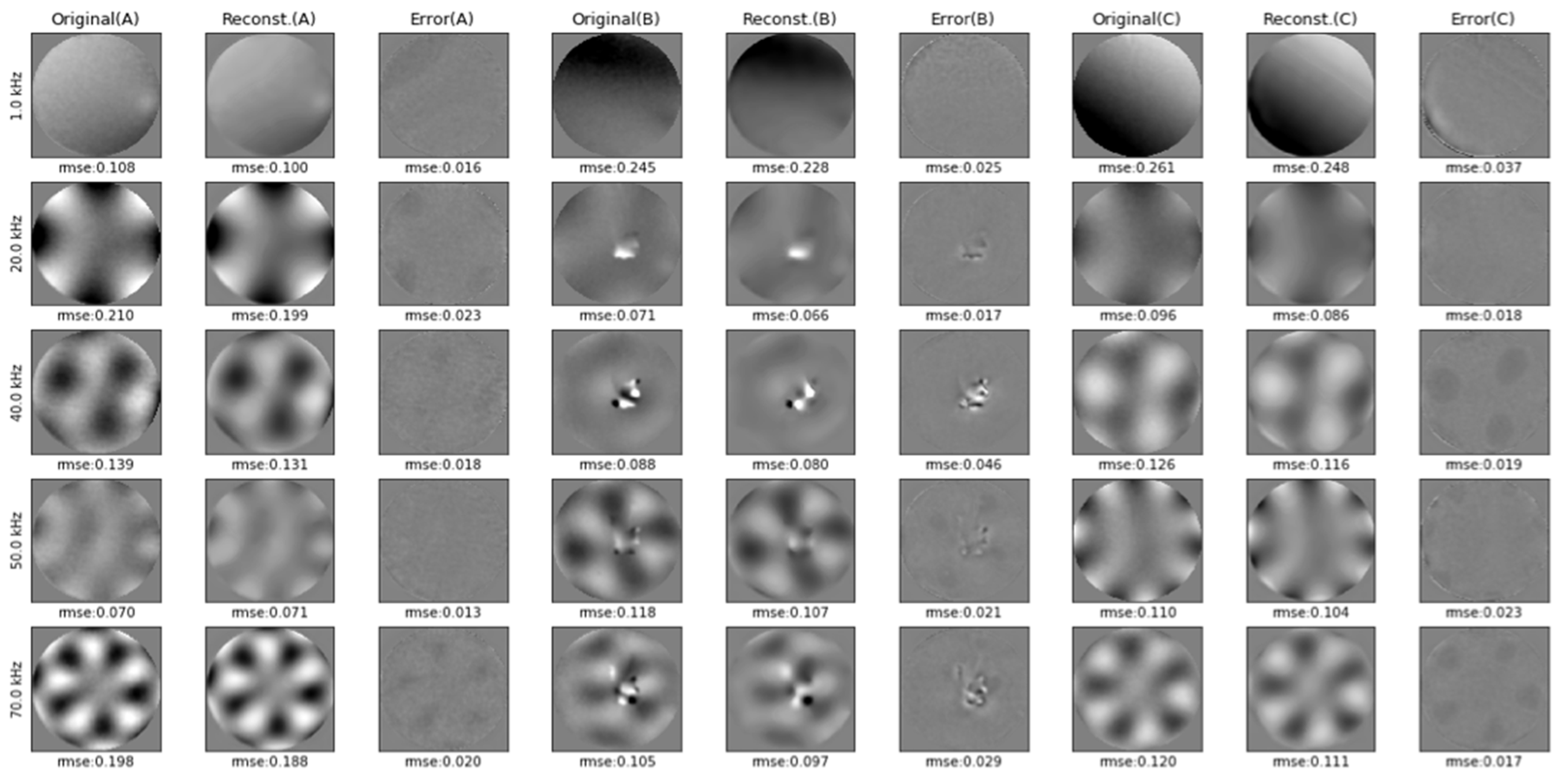
Auto-encoders are the neural architecture that is applicable to anomaly detection for images [17]. Auto-encoders generally have two parts of neural networks called encoders and decoders (Figure 2). For our purposes, the encoder inputs are the images of the normal, or non-damaged, vibration modes. The encoder outputs tensors that retain sufficient information to cope with the task. The decoder reconstructs and outputs an image similar to the original vibration mode from the tensors the encoder outputs. The task of both the encoder and the decoder is to regenerate the original images as closely as possible. The loss is the difference between the reconstructed image and the image from the original vibration mode. We usually take the mean squared error between the two images as the loss function. Both the encoder and the decoder are trained to minimize the loss.

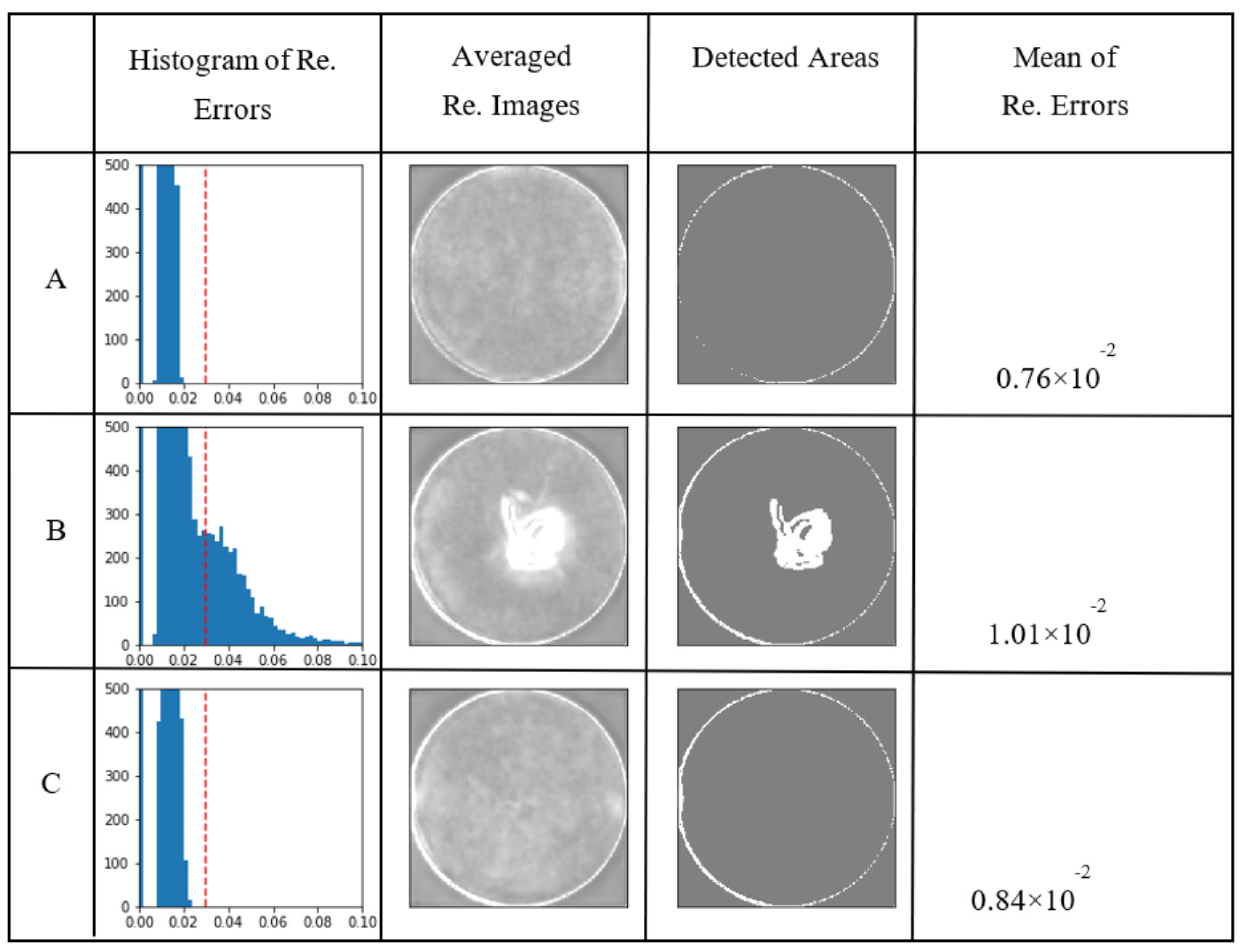
We call the tensor between the encoder and the decoder the tensor representation. The size of the tensor representation is smaller than that of the original images. This setting makes the tensor representation the funnel of information. Being the bottleneck forces the tensor representation to lose insignificant information that is rarely contained in the images of the dataset, which is the set of regular vibration modes. As a result, if the input image has some irregular patterns of vibration modes, the trained network is not able to regenerate it correctly. Its reconstruction error mostly becomes larger because the tensor representation filters information that comes from the irregularity. By measuring the reconstruction errors, we can estimate the extent of the irregularity of input patterns.

3.2. Convolutional Auto-Encoder for Detecting Irregular Patterns

Instead of using fully connected layers in auto-encoders, we use convolutional layers for both the encoder and the decoder [18] (Figure 2). The convolution operation of each single layer has advantages in capturing local features rather than taking all input signals into account. Convolution operations are especially suitable for our purpose because the regular vibration patterns have local and low-level characteristics rather than global features. In the encoder, the convolutions do not change the size of the input images. On the other hand, the down-sampling operations reduce the size of the input to encourage the output tensors to dispose of unimportant information. By repeating convolutions and down-samplings, the encoder can obtain sophisticated embedding vectors that have efficient information. Since the purpose of our network is to reconstruct the regular patterns of inputs, we do not insert any fully connected layers in the network, although the final layer of the encoder is usually preset to a fully connected layer [19]. Thus, our tensor representation is a third-order tensor rather than a vector.

The hyperparameters and the detailed settings of the convolutional auto-encoder are shown in

Table 1. Hyperparameters and detailed settings for convolutional auto-encoder.

Parameters	Encoder	Decoder
# convolutional layers	10	10
# up-/down-samplings	5	5
Input shape	(225, 225, 1)	(7, 7, 256)
Output shape	(7, 7, 256)	(225, 225, 1)
Activate function	Rel	Rel
Up-/down-sampling	max pooling	interpolation
Batch normalization	on each layer	on each layer
Dropout	none	none

# denotes “the number of”.

. The value of each pixel in the input image represents the z-axis displacement of a given vibration mode. The image is processed by ten convolutional and five down (or up) sampling layers in each sub-network. Each sampling layer approximately halves (or doubles) the scale of the input image. Two convolutional layers and a sampling layer are applied alternately. The tensor representation of this convolutional auto-encoder has the shape of 7 × 7 × 256, which is the bottleneck of the whole network. The training dataset consists of vibration modes measured on non-damaged specimens for all the frequencies within a given range, e.g., 1–100 kHz. The signals are normalized so that the means are 0 and the standard deviations are 1. The normalization is completed for both the XY plane and the frequencies within the given range, because the mean of the displacements significantly increases when the frequency is close to a resonance frequency.

3.3. Generating Training Data

The proposed auto-encoder is trained using normal patterns of vibration modes in the data set as mentioned above. Since a sufficiently large amount of data are generally required for training neural networks, a similar number of specimens is usually required as well for stable training. Fortunately, because various patterns of vibration modes are observed by changing the frequency, a sufficiently large number of samples can be obtained from only a few normal specimens prepared for making the dataset. In fact, in the experiments in this paper, auto-encoders are trained only from the data collected from a single normal specimen. We measure vibration modes while increasing the frequency within a given range and add them to the dataset. For instance, suppose that we need to make 1000 samples as the dataset for training and to observe the vibration modes for the frequency band within the range of 1–100 kHz. After slicing the bandwidth of 1–100 into 1000 at regular intervals, the vibration mode is measured at each frequency. The obtained 1000 vibration modes have various different patterns despite that they are observed from a single specimen. As long as the specimen is normal, those patterns are homogeneous and unique with respect to regularity.

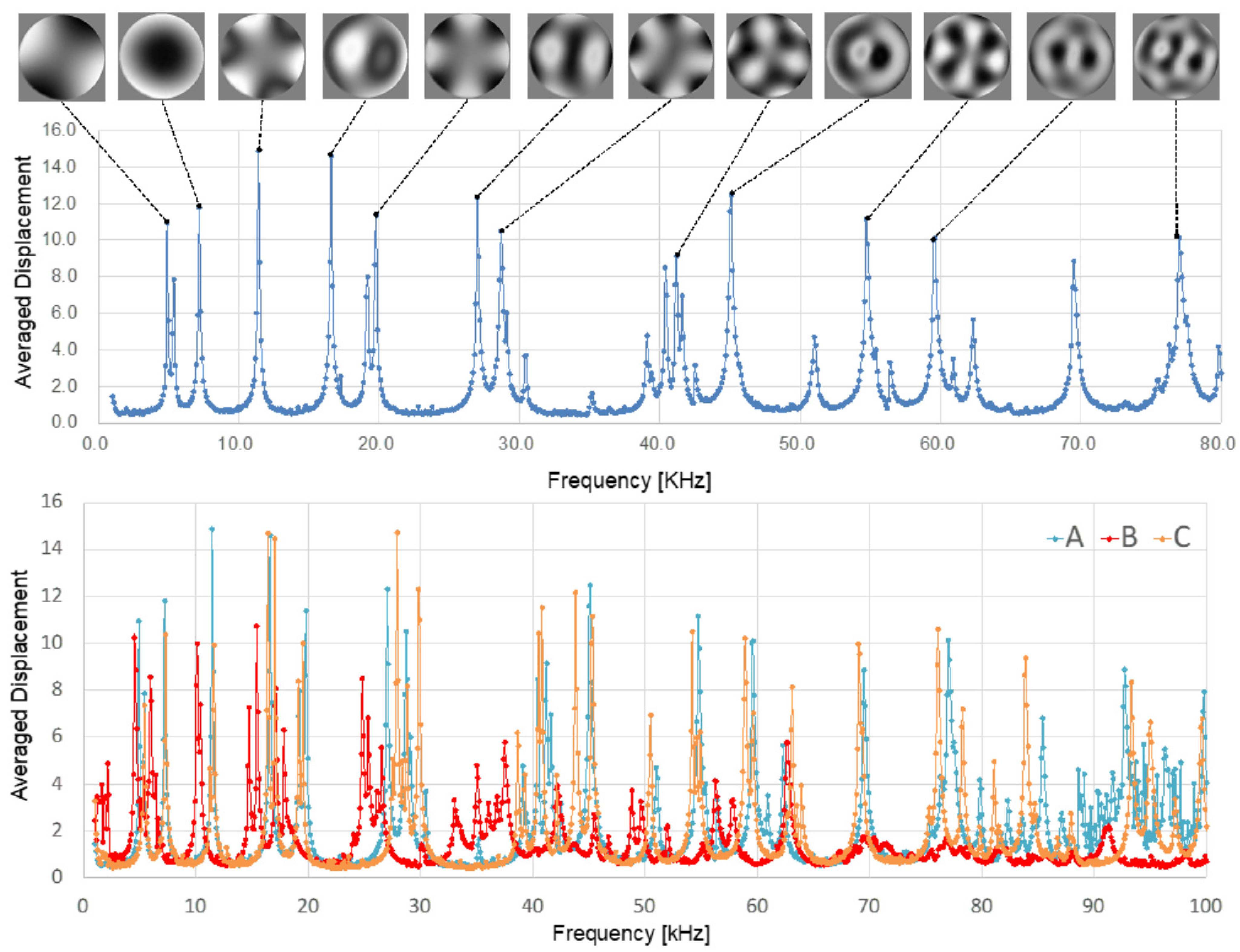
Figure 3 shows the averaged displacement of the vibration mode as a function of the vibration frequency. The data are obtained from a normal circular disk-shaped specimen (see Section 4.1). Peaks in the graph indicate resonance. It can be seen that each resonant frequency has a completely different waveform. Because the pattern changes continuously when we change the frequency, vibration modes that are not resonant also have various patterns. Changing the frequency enables us to successfully obtain various different patterns where normal specimens are characterized. As the images in Figure 3 (top) show, every mode forms a pattern that has some common unique characteristics, which are implicitly learned by training the model. Since a non-damaged specimen should have these characteristics, the reconstruction error tends to be sufficiently small. This fact makes it possible to use the reconstruction error as a measure of irregularity for all specimens, even if they do not have the same vibration modes as the specimen that is used for obtaining the training data.

On the other hand, Figure 3 (bottom) shows the difference in resonance frequencies for different specimens. As shown in the figure, it is not easy to infer whether a specimen is damaged or not from the resonance frequency alone. The shapes of specimens and the average physical properties of them significantly affect their resonance conditions. Slight differences in thickness, shape, etc., can change the distribution of the resonance frequencies. In addition, it is unknown to what extent damage to a small part of the specimen affects the resonance. Even if the change of the resonance frequencies can be calculated by simulation from the detailed observations of damage, it is still unfeasible to identify the damaged area from the distribution of the resonance frequencies because of the difficulty of inverse problems.

3.4. Advantages of Proposed Method

We emphasize that one of the advantages of the proposed method is that we do not need to prepare a large number of specimens. Since a large number of sample images can be obtained by changing the frequency, deep neural networks that are sufficiently accurate for the purpose of detecting damages can be trained from a small number of specimens. In addition, although the time required for detection depends on the performance of computers or GPUs, it can be completed in a few milliseconds per image with a typical high-performance GPU. Therefore, even if a couple of hundred frequency scans are required, the total computation time is less than one second.

4. Experiments

4.1. Composite Material and Damaged Specimen Preparation

Short carbon fiber-carbon matrix composite dispersed Si/SiC matrix (hereafter denoted as “(C/C)/Si/SiC”) composites used in this study were fabricated through reactive liquid silicon melt infiltration (RMI) process, described elsewhere [7]. A fabricated composite disk (density ~2.4 g/cm³) was supplied by CoorsTek Co., Ltd. (Tokyo, Japan). Pitch-based short carbon fiber bundle (DIALEAD^®, K-223HG, Mitsubishi Plastics Inc., Tokyo, Japan), which had a typical length of ~6 mm, was used as a reinforcement of C/C and C/SiC phases. The number of fibers per unit bundle was 12,000 fibers. The content of carbon fiber in the entire composite was ~30 vol%. Figure 4 shows polished sections of the composite, both parallel and perpendicular to through-thick-direction. (C/C)/Si/SiC consists of four major phases; C/C, Si, SiC, and C/SiC [7]; C/C composite phase is distributed in an in-plane quasi three-dimensionally random manner. The selected mechanical properties of this composite are listed in

Table 2. Mechanical properties of composite material that specimens were made from.

Mechanical Property	Value
Density, ρc (g/cm3)	2.4
Young’s modulus, Ec (GPa)	5–10
Tensile strength, σc (MPa)	35–50
Poisson’s ratio, νc	0.2

.

The fabricated composite was cut into disk-shaped impact test specimens, each of which had a circular disk shape with a diameter of 80 mm and a thickness of 5 mm. The parallel surfaces of the specimen were polished up to 1 μm with a diamond paste finish. A drop weight impact test was carried out using a drop weight impact testing machine (Instron Corp., Dynatup Model 8250, Norwood, MA, USA). Details of the same instruments are shown in the reference [20]. The disk-shape specimen was clumped to a specimen support, which had a circular hole (50 mm diameter) in the center, to avoid free vibration after onset of impact. This clamping was effective to avoid specimen vibration during and after impact. Used impact test conditions, impact tip, height and impact energy are listed in

Table 3. Overview of impact loading tests on specimens.

Specimen	Impact Tip (in.)	Height (m)	Velocity (m/s)	Initial Energy (J)	Propagation Energy (J)
Damaged B	0.50	0.178	1.867	1.545	6.712
Damaged C	0.25	0.057	1.059	2.208	3.073

. A tip diameter of the used indenters was 0.5 or 0.25 inches. The experimental range was selected based on a set of preliminary experiments of the same (C/C)/Si/SiC composite. Impact speed of the indenter is simply obtained from $\upsilon =\sqrt{2gh}$, where $h$ is the height of indenter tip and $g$ is the acceleration of gravity (9.8 m/s²). The conditions were chosen to introduce characteristic damage behaviors of the present (C/C)/Si/SiC composite under service conditions.

After the tests, the impact and back surfaces were observed by an optical microscope. Damage evolution on the impact surface and inside the specimen was carefully observed. Scanning electron microscopy (SEM) was also performed on some impact-tested specimens. In the present study, specimens with three different conditions were used: (a) original un-damaged, (b) damaged with υ = 1.867 m/s, (c) damaged with υ = 1.059 m/s. Figure 5 shows the examples of the impact surfaces of (C/C)/Si/SiC composite. It is clear that micro-scale crack extension from near the center of the specimen is observed in the back surface observed by SEM (Figure 5c’) as indicated by the arrows. It should be noted that only small microcracks, the lengths of which are smaller than 1 mm, occur with the impact speed of 1.059 (υ = 1.059 m/s). However, this damage is difficult to observe from the back surface. This difficulty is due to the random formation of microcracks in the entire specimen. Detailed impact damage of (C/C)/Si/SiC is beyond the scope of this paper and the behavior will be reported elsewhere [7]. On the contrary, a large crack is observed at the back surface of the other impact-tested specimen (Figure 5b’). The out-of-plane deformation on the back surface of the specimen is clearly observed near the center. It can be seen that the major cracks spread from the impact point by observing their angles as indicated by the arrows in Figure 5b. It is considered that the behavior is associated with the impact damage accumulation through the formation of microcracks and delamination dependent microstructure of the composite.

The surface damage evolution was characterized using Electronic Speckle Pattern Interferometry (ESPI), which has been applied to measure the change of vibration amplitude for NDE. The measurement of the vibration patterns was carried out using ESPI (VibroMap 1000. Optonor, Inc., Trondheim, Norway). Experimental setup is shown in Figure 6. The specimen was set up on the soft material to avoid external vibrations. The light source used was a 150 mW Nd:YAG laser with a wavelength of 532 nm. A laser beam illuminated the back surface of the specimen after the impact test. Specimens were excited dynamically by a piezoelectric sound (FGT-15T-6.0A1W40, Universal Electronics Co., Ltd., Scottsdale, AZ, USA) mounted on the impacted surface near the outer circumference of the specimen. Vibration patterns were measured by exciting the specimen in the frequency range of 1 to 104 kHz with 0.1 kHz increments. A total of 1040 images were obtained to apply AI technology each for the specimens. The averaging filters were applied to the vibration modes to remove the high-frequency speckle noise.

4.2. Dataset Preparation and Training Models

We used the specimen in the state (a) to obtain training data. The range of vibration frequency is 1–104 kHz, where a sufficient variation pattern is actually observed. The section is split into 0.1 kHz increments. A total of 1040 images are obtained. The input image has a resolution of 225 × 225. Each pixel represents the value of displacement normalized so that the mean is 0 and the variance is 1.

The convolutional autoencoder is trained using the 1040 images obtained from (a) as training data. The loss function is the reconstruction error, that is, the rooted mean squared error (RSME) of the difference between the input image and the output image of the convolutional auto-encoder model, as described in Section 3.2. Adam is used for the optimization of the model. Training was carried out for 100 epochs. The batch size is 64. In order to reduce the reconstruction error, we did not apply dropout and instead applied batch normalization in each convolutional layer. Hyperparameters, such as batch size and number of epochs, were set arbitrarily within the range where learning is stable. For the autoencoder, both the encoder and decoder are 3-layer fully-connected neural networks, and the dimensionality of the vector representation connecting the encoder and decoder is 4096.

Apart from the training data, the datasets obtained from specimens (b) and (c) are used as the verification data. Similar to (a), 1040 images are obtained from frequencies within 1–104 kHz. By inputting each of the 1040 images of (b) (or (c)) to the trained model, its reconstruction error is calculated.

5. Results of Experiments

5.1. Results of Anomaly Detection for a Given Frequency

As described above, three specimens are prepared, one of which is used for learning (a), and the other two are used for testing ((b), (c)). In this section, we examine to what extent much damage can be detected from the reconstruction errors for a given frequency. The original vibration modes (the column label is “Original” in Figure 7), the reconstructed images (“Reconst.”), and the reconstructed errors (“Error”) when the vibration frequencies are preset to 1, 20, 40, 50, and 70 kHz are shown in Figure 7. The left three columns, the middle three columns, and the right three columns show the results for specimens (a), (b), and (c), respectively. By observing the columns with the reconstruction error images (third, sixth, and ninth columns from the left), we can recognize whether the damaged area has been successfully detected. The color of the image is black if the reconstruction error is −1 or less, and white if the reconstruction error is +1 or more. Gray means that the reconstruction error is close to zero. From the images in the third column in Figure 7, it can be seen that for specimen (a), the reconstruction error is close to 0 at any frequency and in any region in the image. This means that no damage was detected for (a) at any frequency, which is not surprising, because (a) is the reference specimen without damage and is used for making the training data. On the other hand, for specimen (b), it can be seen that at some frequencies (at 20 and 40 kHz), the reconstruction errors are clearly not close to 0 around the center. For other frequencies, the reconstruction errors are almost 0, however. We can see that the damaged area is detected depending on the vibration frequency. For specimen (c), since the reconstruction errors are almost 0 for all frequencies and regions, we can conclude that the damaged area is not detected at any frequency.

From the viewpoint of mm-order NDEs, it is ideal that a damaged area is detected only for (b), as will be described later. The experimental results indicate that the proposed method evaluates damage correctly and detects the concerning area precisely. However, as shown in Figure 7, the detection of damage depends on vibration frequencies. The multiple images of the reconstruction errors need to be integrated into one image since vibration frequencies should not affect the result of the detection. In addition, for automatic detection, it is better to generate a binary image where each pixel represents whether it is damaged or not. In Section 5.2, the integration and binarization are addressed for more interpretable and quantitative evaluation.

5.2. Results of Dataset Preparation and Training Models

Reconstruction errors measured from a specimen should be processed so that all of them are integrated with respect to frequency and converted into a binary image where each pixel represents if it is in a damaged area or not. We define a procedure as follows:

• First, in order to eliminate the difference between frequencies, we average the absolute values of reconstruction errors for all frequencies. We call the obtained image the mean absolute reconstruction errors (MAREs). In addition, we make a histogram of the MAREs;
• Second, a threshold for the MAREs is determined from the histogram for the reference specimen used for training (specimen (a)). Here, we define a threshold by adding a margin to the max value of the MAREs. Since the damaged area must not be detected in any images of the reference specimen, the threshold is needed to be larger than the max of the MAREs of the reference specimen, at least;
• Finally, the MAREs for the testing specimen are binarized using the threshold obtained in (2). Note that we can control the sensitivity of detection by changing the margin described in (2).

Figure 8 shows the results of binarizing the MAREs obtained by the trained proposed model, where the threshold is set to 0.03. In the histograms of the MAREs of specimens (a) and (c), all pixels are clearly below the threshold. As the histograms in Figure 8 show, their distributions are concentrated around 0.01–0.02. On the other hand, for specimen (b), we observe a distribution that has a long tail, which is clearly different from the distributions of the histograms for (a) and (c). Most of the area of the tail exceeds the threshold and is detected as a damaged area. The detected area coincides with the true damage area as described in Section 4.2.

Figure 9 shows the results using a simple autoencoder consisting of fully-connected layers only. Although the true damage area is successfully detected for specimen (b), some foggy damaged areas, which are false, are also detected for specimen (c) wrongly. This is because the overall reconstruction errors in (c) tend to be large, as seen from the histogram of the MAREs. This fact indicates that the model is overfitted to specimen (a), which is used for making the training data. On the other hand, with respect to the histograms of the proposed neural network, specimen (c) has almost the same distribution as specimen (a), indicating that the proposed network is superior to the simple auto-encoder in terms of damage detection.

6. Conclusions

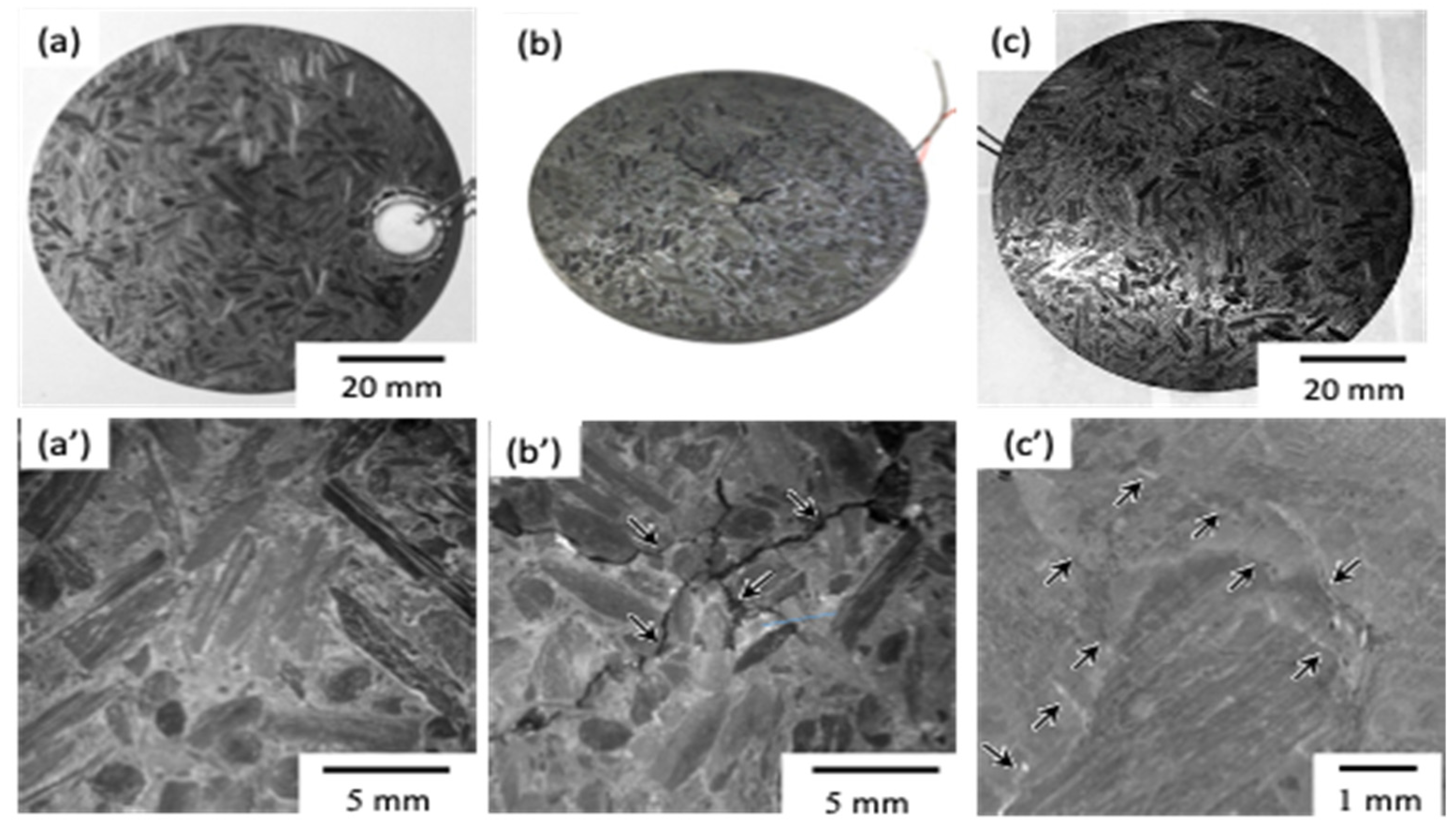
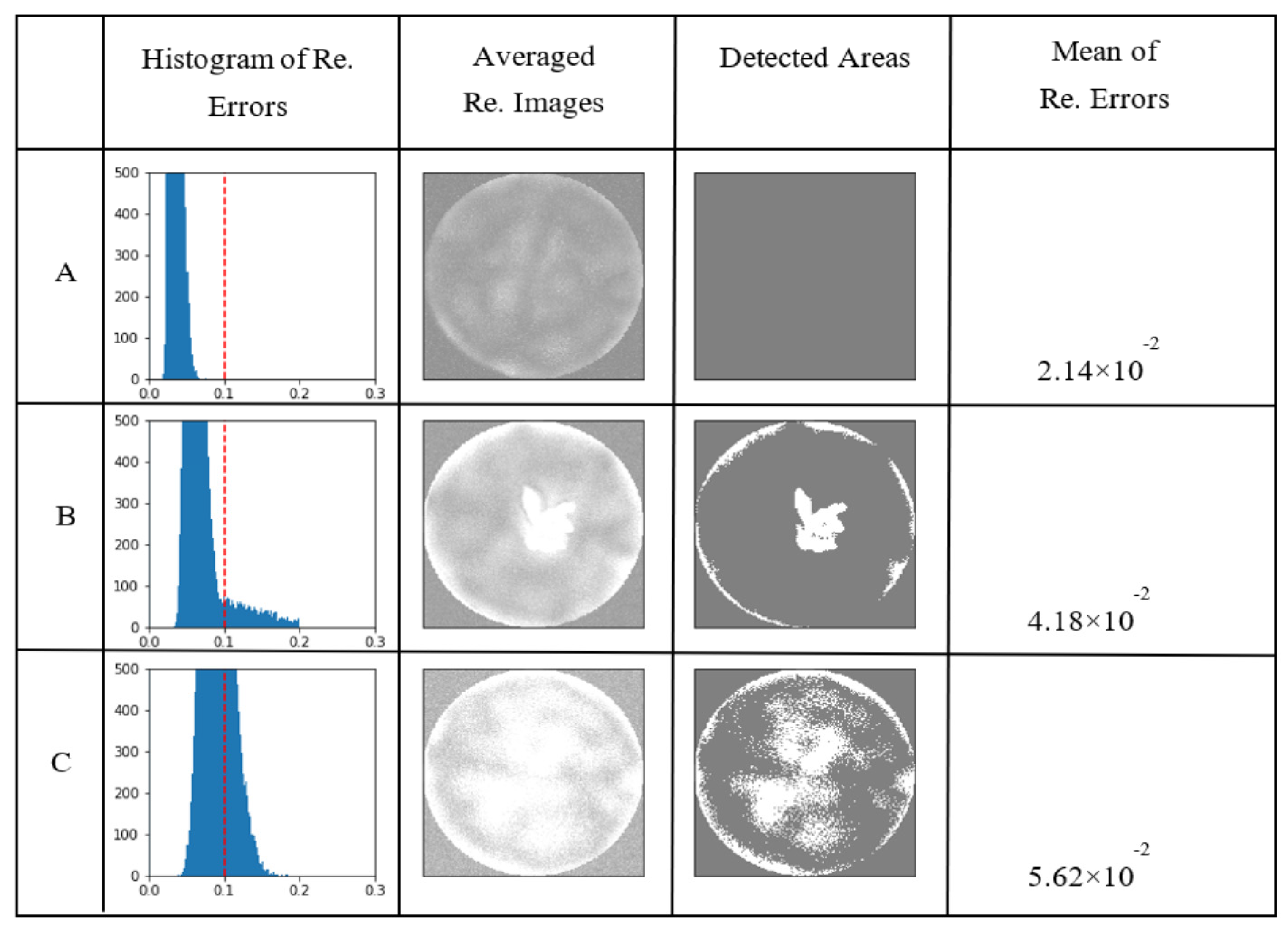
The experiments in this paper demonstrated that the proposed method detected the damaged area correctly and precisely for the verification specimens (b) and (c) from the viewpoint of macroscopic-level evaluation, which is the purpose of the NDE using vibration mode (see Section 2). Since the scale of the microscopic-level damage is beyond the expected scale that the proposed NDE method is supposed to cover, it is consistent with the experimental results that our method does not detect any area in specimen (c), which has only small cracks (see the discussion in Section 4.2). The main contribution is that, despite the fact that we use only a single specimen for training, we succeed in detecting the damaged area fairly accurately using methods of deep learning, which generally require us to prepare a large amount of data. On the other hand, the fact that there are only two verification specimens is a point to be further examined in the future.

Micro-level defects such as cracks/damage/pores, which are difficult to observe visually, may affect the physical properties of the material after being accumulated. If some outliers occur in the physical properties of the specimen, such as stiffness, the anomaly area may be detected as a damaged area with our method. It is necessary to examine in the future what kind of micro-level defects and to what extent they accumulate to cause significant changes in the physical properties.

References

1. Krenkel, W.; Heidenreich, B.; Renz, R. C/C-SiC Composites for Advanced Friction Systems. Adv. Eng. Mater. 2002, 7, 427–436. [Google Scholar] [CrossRef]
2. Rentz, R.; Seifert, G.; Krenkel, W. Interration of CMC brake disks in automotive brake systems. Appl. Ceram. Technol. 2012, 9, 712–724. [Google Scholar] [CrossRef]
3. El-Hija, H.A.; Krenkel, W.; Hugel, S. Development of C/C-SiC Brake Pads for High Performance Elevators. Int. J. Appl. Ceram. Technol. 2005, 2, 105–113. [Google Scholar] [CrossRef]
4. Bansel, N.P. (Ed.) Carbon Fiber Reinforced Silicon Carbide Composites (C/SiC, C/C-SiC). In Handbook of Ceramic Composites; Springer: Boston, MA, USA, 2005; pp. 117–148. ISBN 9780387239866. [Google Scholar]
5. Goto, K.; Kagawa, Y. Fracture Behavior and Toughness of a Plane-Woven SiC Fiber-Reinforced SiC Matrix Composite. Mat. Sci. Eng. 1996, A211, 72–81. [Google Scholar] [CrossRef]
6. Sakai, M.; Brad, R.C. Fracture toughness testing of brittle materials. Int. Mat. Rev. 1993, 38, 53–78. [Google Scholar] [CrossRef]
7. Inoue, R.; Yang, J.; Kakisawa, H.; Kagawa, Y. Mode I fracture toughness of short carbon fiber-dispersed SiC matrix composite fabricated by melt infiltration process. Ceram. Int. 2013, 39, 8341–8346. [Google Scholar] [CrossRef] [Green Version]
8. Inoue, R.; Yang, J.-M.; Kakisawa, H.; Kagawa, Y. Mixed-Mode Fracture Criterion of Short Carbon Fiber-Dispersed SiC Matrix Composite. J. Ceram. Sci. Technol. 2017, 8, 223–232. [Google Scholar]
9. Zhu, Y.-K.; Tian, G.-Y.; Lu, R.-S.; Zhang, H. A Review of Optical NDT Technologies. Sensors 2011, 11, 7773–7798. [Google Scholar] [CrossRef] [PubMed] [Green Version]
10. Sun, J. Evaluation of Ceramic Matrix Composites by Thermal Diffusivity Imaging. Int. J. Appl. Ceram. Technol. 2007, 4, 75–87. [Google Scholar] [CrossRef]
11. Shichijo, N.; Takeshima, Y.; Matsuoka, J.; Kano, T.; Kagawa, Y. Automated Structural Recognition and Evaluation of CMCs using Deep Neural Networks. In Proceedings of the 10th International Conference on High Temperature Ceramic Matrix Composites, Bordeaux, France, 22–26 September 2019. [Google Scholar]
12. Schmidt, C.; Hocke, T.; Denkena, B. Artificial intelligence for non-destructive testing of CFRP prepreg materials. Prod. Eng. 2019, 13, 617–626. [Google Scholar] [CrossRef]
13. Ruff, L.; Kauffmann, J.R.; Vandermeulen, R.A.; Montavon, G.; Samek, W.; Kloft, M.; Dietterich, T.G.; Muller, K.-R. A Unifying Review of Deep and Shallow Anomaly Detection. Proc. IEEE 2021, 109, 756–795. [Google Scholar] [CrossRef]
14. Pang, G.; Shen, C.; Cao, L.; Hengel, A.V.D. Deep Learning for Anomaly Detection: A Review. ACM Comput. Surv. 2021, 54, 1–38. [Google Scholar] [CrossRef]
15. Ronneberger, O.; Fischer, P.; Brox, T. U-Net: Convolutional Networks for Biomedical Image Segmentation. In Model Checking and Artificial Intelligence; Springer: Singapore, 2015; pp. 234–241. [Google Scholar]
16. Tan, M.; Le, Q. Efficient Net: Rethinking Model Scaling for Convolutional Neural Networks. In Proceedings of the 36th International Conference on Machine Learning, Long Beach, CA, USA, 10–15 June 2019. [Google Scholar]
17. Sakurada, M.; Yairi, T. Anomaly Detection Using Autoencoders with Nonlinear Dimensionality Reduction. In Proceedings of the MLSDA 2014 the 2nd Workshop on Machine Learning for Sensory Data Analysis, Gold Coast, Australia, 2 December 2014; p. 4. [Google Scholar]
18. Masci, J.; Meier, U.; Cireşan, D.; Schmidhuber, J. Stacked Convolutional Auto-Encoders for Hierarchical Feature Extraction. In Advances in Autonomous Robotics; Springer: Dordrecht, The Netherlands, 2011; pp. 52–59. [Google Scholar]
19. Dizaji, K.G.; Herandi, A.; Deng, C.; Cai, W.; Huang, H. Deep Clustering via Joint Convolutional Autoencoder Embedding and Relative Entropy Minimization. In Proceedings of the 2017 IEEE International Conference on Computer Vision (ICCV), Venice, Italy, 22–29 October 2017; pp. 5747–5756. [Google Scholar]
20. Ramirez, B.J.; Gupta, V. Energy Absorption and Low Velocity Impact Response of Open-Cell Polyurea Foams. J. Dyn. Behav. Mater. 2019, 5, 132–142. [Google Scholar] [CrossRef] [Green Version]
Figure 1. Target resolution for NDE using vibration/resonance modes.
Jcs 05 00301 g001
Figure 2. Detection of irregular patterns using convolutional auto-encoder.
Jcs 05 00301 g002
Figure 3. (top) Variation of vibration modes obtained from a single specimen. (bottom) The comparison of peak frequencies between specimens; A: undamaged specimen (no impact test), B and C: specimens subjected to impact test.
Jcs 05 00301 g003
Figure 4. A typical example of (C/C)Si/SiC composite: (a) the overview of the specimen, (b) parallel, and (c) perpendicular to through-thick-direction.
Jcs 05 00301 g004
Figure 5. A typical example of impact-tested surface of (C/C)Si/SiC composite: (a) original un-damaged, (b) damaged B, and (c) damaged C, (a’c’) detail of the back surface around center.
Jcs 05 00301 g005
Figure 6. Schematic illustration of an ESPI system.
Jcs 05 00301 g006
Figure 7. Inputs, outputs, and reconstruction errors for specimen (a), (b), and (c). (AC) corresponds to specimen (a), (b), and (c), respectively.
Jcs 05 00301 g007
Figure 8. Detection of the irregular area using convolutional auto-encoder (proposed model). (AC) corresponds to specimen (a), (b), and (c), respectively.
Jcs 05 00301 g008
Figure 9. Detection of irregular areas using auto-encoder. (AC) corresponds to specimen (a), (b), and (c), respectively.
Jcs 05 00301 g009