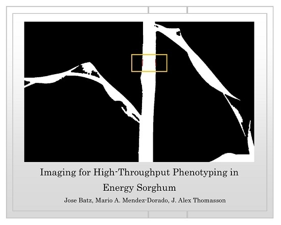
Imaging for High-Throughput Phenotyping in Energy Sorghum

Abstract

The increasing energy demand in recent years has resulted in a continuous growing interest in renewable energy sources, such as efficient and high-yielding energy crops. Energy sorghum is a crop that has shown great potential in this area, but needs further improvement. Plant phenotyping—measuring physiological characteristics of plants—is a laborious and time-consuming task, but it is essential for crop breeders as they attempt to improve a crop. The development of high-throughput phenotyping (HTP)—the use of autonomous sensing systems to rapidly measure plant characteristics—offers great potential for vastly expanding the number of types of a given crop plant surveyed. HTP can thus enable much more rapid progress in crop improvement through the inclusion of more genetic variability. For energy sorghum, stalk thickness is a critically important phenotype, as the stalk contains most of the biomass. Imaging is an excellent candidate for certain phenotypic measurements, as it can simulate visual observations. The aim of this study was to evaluate image analysis techniques involving K-means clustering and minimum-distance classification for use on red-green-blue (RGB) images of sorghum plants as a means to measure stalk thickness. Additionally, a depth camera integrated with the RGB camera was tested for the accuracy of distance measurements between camera and plant. Eight plants were imaged on six dates through the growing season, and image segmentation, classification and stalk thickness measurement were performed. While accuracy levels with both image analysis techniques needed improvement, both showed promise as tools for HTP in sorghum. The average error for K-means with supervised stalk measurement was 10.7% after removal of known outliers.

1. Introduction

In this age of increasing concerns about population growth, energy demands and environmental risks, the need to expand energy resources in a sustainable manner is intensifying. Non-renewable energy from fossil fuels will be insufficient at a certain point in the future [1,2]. Additionally, carbon dioxide emissions from fossil fuels have led to concerns about rising levels of greenhouse gases [3], increasing the importance of developing alternative energy sources, like dedicated energy crops that reduce net carbon dioxide emissions. One solution to these issues is to increase energy crop production by maximizing crop output per unit area.

Improving crop productivity is possible through improvements in breeding and genetics. Historically, breeders and geneticists relied on manual labor to evaluate crop physical traits (phenotypes) on a relatively small number of plant varieties. The advent of sensing and robotics has provided the potential to drastically accelerate the advances of breeding and genetics through “high-throughput phenotyping” (HTP). This new research field involves using autonomous technologies to rapidly and accurately measure phenotypes on a large number of plants, enabling the selection of promising varieties and genes from a broader genetic pool to make faster strides in crop improvement. With dedicated energy crops, the most important phenotypes are biomass yield, rate of growth and resistance to typical crop stresses.

Certain crops like sorghum (Sorghum bicolor) have been demonstrated to have excellent potential for dedicated bioenergy production. Sorghum is a C4 plant with a high biomass accumulation rate, and it can be economically produced and harvested in four months or less with suitable environmental conditions [3,4,5]. While some varieties of sorghum are grown mainly for grain (grain sorghum), others are grown mainly for the sugars they produce (sweet sorghum) or for their high levels of biomass (forage sorghum or “energy sorghum”) [6].

Plant breeders can potentially accelerate biomass production improvements in energy sorghum by using an HTP approach. Previous studies have pursued automation of phenotype-measurement techniques involving lasers, light curtains, ultrasonic sensors and artificial vision [7,8,9]. The use of phenotypic data along with genotypes of energy sorghum has been reported in a few recent studies [10,11,12,13]. Artificial vision systems are able to extract meaningful information from images, such as qualitative and quantitative morphologic variables [14], like plant height, width and shape, stem diameter and leaf number, area and angle. There is also the potential to use spectral characteristics in images to measure plant health, such as by correlating greenness to chlorophyll content [15,16,17,18]. Machine vision is potentially faster, more reliable and more robust than manual phenotyping methods [19]. A needed development in machine vision is the capability of working under difficult imaging conditions, like varying light levels, spectra and angles in crop fields, as well as varying temperature, etc. [20].

In a dedicated energy crop like energy sorghum, stalk thickness and plant height are the most significant phenotypes correlated to biomass, because a large majority of the plant dry matter resides in the stalk. Plant height can be measured with ultrasonic sensors, but an automated measuring system for stalk thickness remains a significant challenge because of the possible occlusion of the stalk and the difficulty of differentiating the stalk from connected stems. Numerous imaging techniques for HTP have been developed, and many are available at the Plant Image Analysis website [21]. Two of the available software resources at that website are Root Estimator for Shovelomics Traits (REST; [22]) and Digital Imaging of Root Traits (DIRT; [23]), both of which are dedicated to the analysis of images to measure root morphology, such as width, depth, length, shape and diameter. Neither of these incorporates measurement of distance between camera and plant material. It is clear that currently available software offers length measurement capabilities for plants, particularly root masses, but the authors are not aware of existing software dedicated to plant stalk measurement, particularly when camera distance is included. The first objective of this research was to evaluate common image analysis techniques as potential tools for measuring stalk thickness that could be used in automated HTP. The second objective was to evaluate an active depth camera as a tool for measuring distance between camera and plant, a measurement that would likely be necessary if an image-based stalk thickness measuring system were to be deployed.

2. Experimental Section

2.1. Materials

2.1.1. Energy Sorghum Material

Two genetic varieties of energy sorghum known as R07019 (Variety A) and R07007 (Variety B) were planted in plastic pots. These varieties have been studied as potential dedicated energy crops by Dr. John Mullet of Texas A&M University and were made available for this phenotyping study. Four plants per variety were planted, two plants to a pot. Each pot was supplied with 17 g of Osmocote 14-14-14 slow release fertilizer (Scotts). The plants were grown under well-watered conditions; i.e., the soil surface was kept moist throughout the experiment. All pots were progressively thinned to 1 plant per pot as the seedlings grew. The pots were placed in a greenhouse where environmental conditions were monitored with a TinyTag Data Logger^© (Gemini Data Loggers). The average daily minimum temperature and relative humidity were 24.1 °C (±1.1 °C) and 36.0% (±14.0%), respectively. The average daily maximum temperature and relative humidity were 32.3 °C (±1.8 °C) and 69.9% (±11.3%). Plants emerged roughly five days after planting and were without branching nodes for the first few weeks. Thus, the first images were collected about three weeks after planting, when the plants began to exhibit thicker stalks and leaves emerging from the stalk.

2.1.2. Camera

An inexpensive (under $200 USD in 2015) combined camera (Creative Technology Ltd., Milpitas, CA, USA, Model VF0780), composed of a standard RGB camera and a 3D active camera (SoftKinetic Inc., Sunnyvale, CA, USA), was used to capture images of the sorghum plants. The 3D camera employs the time-of-flight (TOF) concept, measuring the time between emitting a pulse of light and receiving the reflected light, to measure depth values in a field-of-view plane. TOF cameras, or “depth cameras”, are commonly composed of a near-infrared (NIR) source and a CMOS pixel-array detector. The depth camera used includes a three-chip TOF system designed to be sensitive only in the 850 to 870-nm range, matching the NIR source. This TOF system provides a 320 × 240 resolution image in which pixel values relate to the distance from image objects to the emitter on the camera. Manufacturer specifications list the depth values’ precision as in the range of 5 to 300 cm, with the best performance from 15 cm to 100 cm. The field of view (FOV) of the RGB and depth cameras is not identical. The RGB camera resolution can be selected from 320 × 240 to 720 × 1280. Initially, 320 × 240 was maintained in the RGB images for consistency with the depth images, but in later stages of plant growth, the RGB resolution was increased to 720 × 1280 for more precise measurements of stalk thickness.

2.1.3. Imaging Environment

A polyvinyl chloride (PVC) pipe frame was built to hold a black cotton cloth to block sunlight in the greenhouse and to aid in isolating sorghum plants from their surroundings, facilitating plant classification during image analysis. The cloth also helped block possible incoming NIR energy that might interfere with the depth camera.

2.2. Methods

Over a period of ten weeks, images and stalk thickness measurements of the sorghum plants were collected on roughly a weekly basis. According to recommendations by Dr. William Rooney of Texas A&M University [24], stalk thickness was to be measured immediately above the plant’s third internode to provide consistent and representative measurements of the entire stalk. In the early stages of growth, sorghum plants did not exhibit internodes, so a measurement height of 7 cm above the soil was used until internodes were defined, a situation that occurred about six weeks after data collection began. Sorghum stalks have a roughly elliptical cross-section, so effective thickness was determined based on an elliptical shape model. Manual thickness measurements were made with a caliper. Both the wider (major-axis) and narrower (minor-axis) dimensions of the stalk were measured for each plant on each data collection date. The wider dimension of the sorghum stalk, which is perpendicular to the direction at which the leaves emerge, was oriented perpendicular to the camera viewing direction. A marker was placed on the pots during the first measurement so that each time measurements were made, the orientation of the plants would be the same. Distance from the camera lens to the background cloth was measured with a ruler to the nearest half cm.

Plants were placed between roughly 25 and 70 cm from the camera, as manually measured with a ruler to the nearest half cm, horizontally from the edge of the camera lens to the center of the sorghum stalk. Distances were varied to provide a range of distances to compare between manual and depth-camera measurements and also, in some cases, to provide adequate distance to image the entire plant. The camera was placed so that the point where caliper measurements were made was just below the image center. In the later stages when plants had developed internodes, the camera was placed so that the third internode was slightly below the center of the image. The camera was horizontally leveled to reduce possible error from image distortion that might occur if the camera were not perpendicular to the plant’s frontal plane.

2.2.1. Image-Distance Calibration

Image-distance calibration consisted of producing a conversion factor from pixels to length units (mm). A 47.6-mm diameter PVC tube was placed in front of the camera at distances from 20 to 90 cm in 10-cm increments, and an RGB image was collected at each distance. The number of pixels belonging to the object at each distance was determined, and an equation was developed to convert pixels to distance. The accuracy of the depth camera measurements was considered independently, and this analysis is considered below.

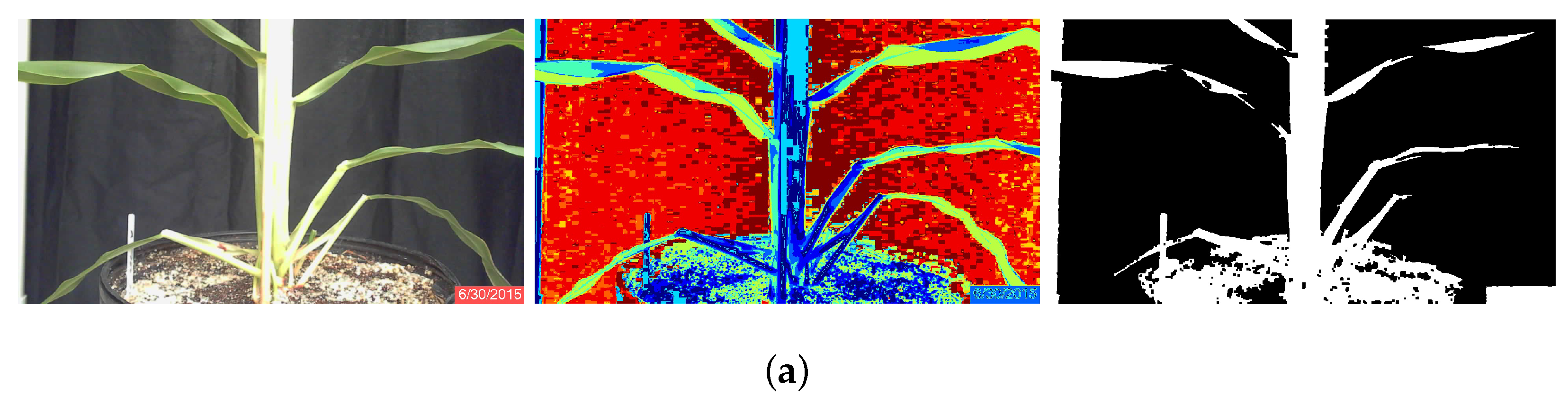
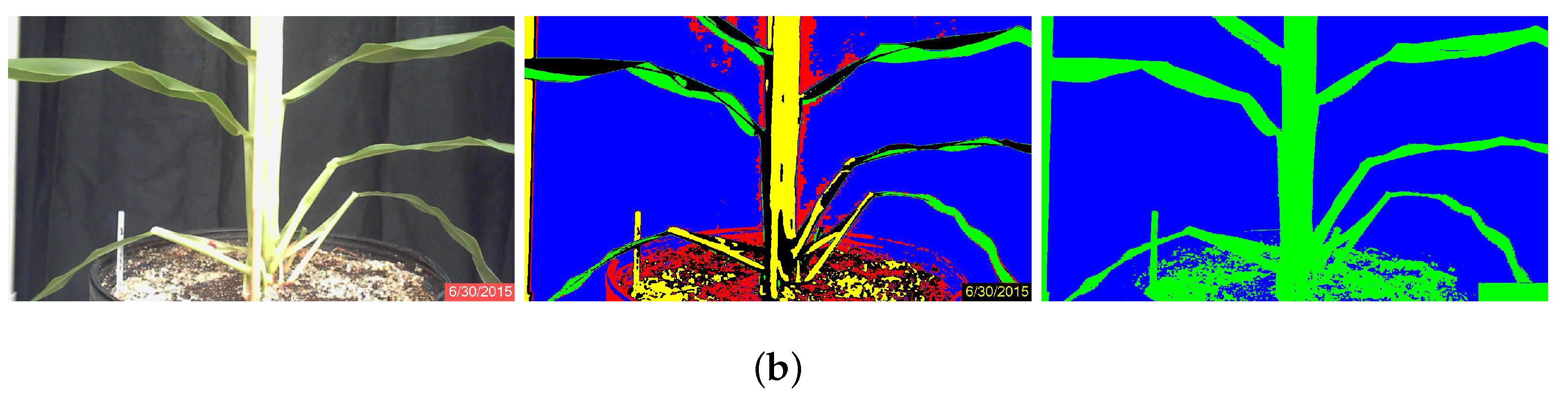
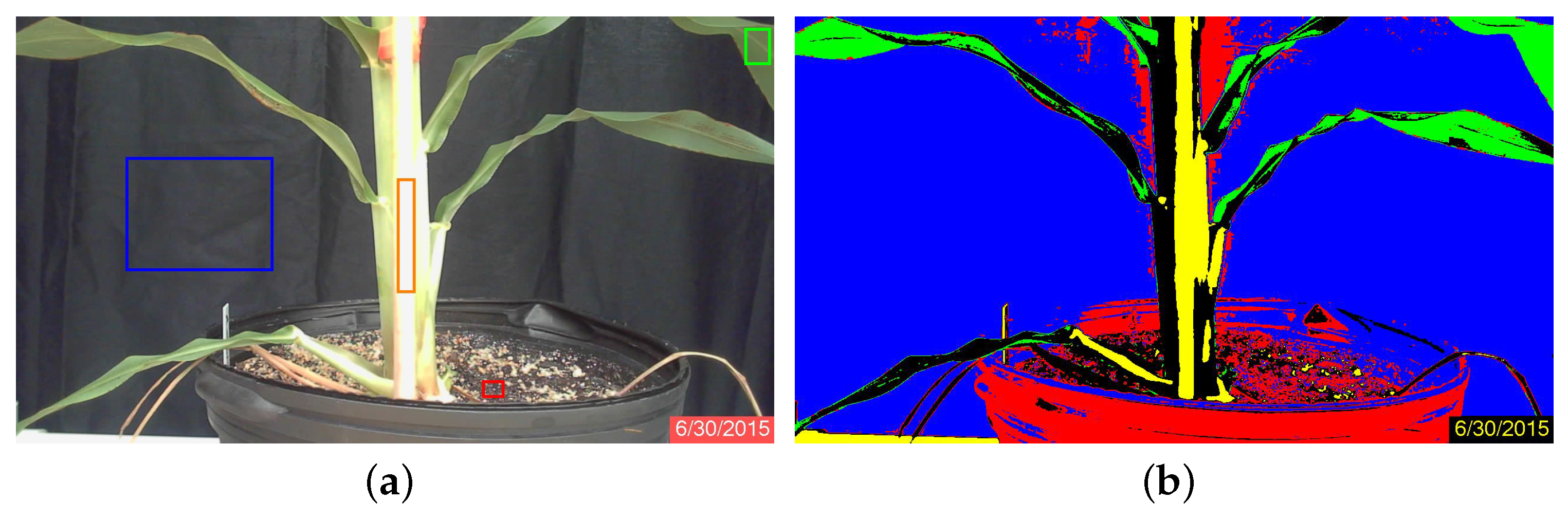
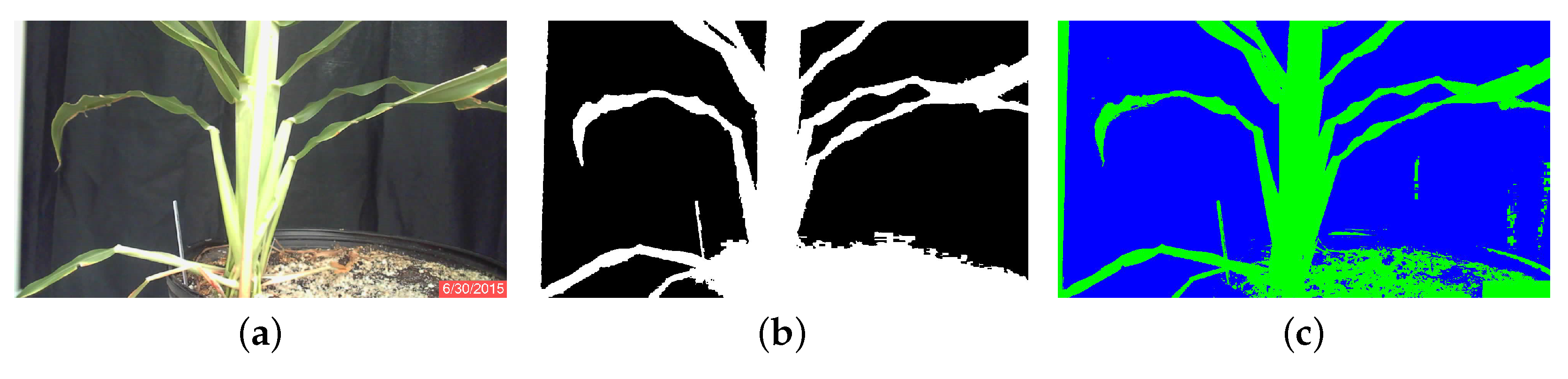
2.2.2. Image Analysis

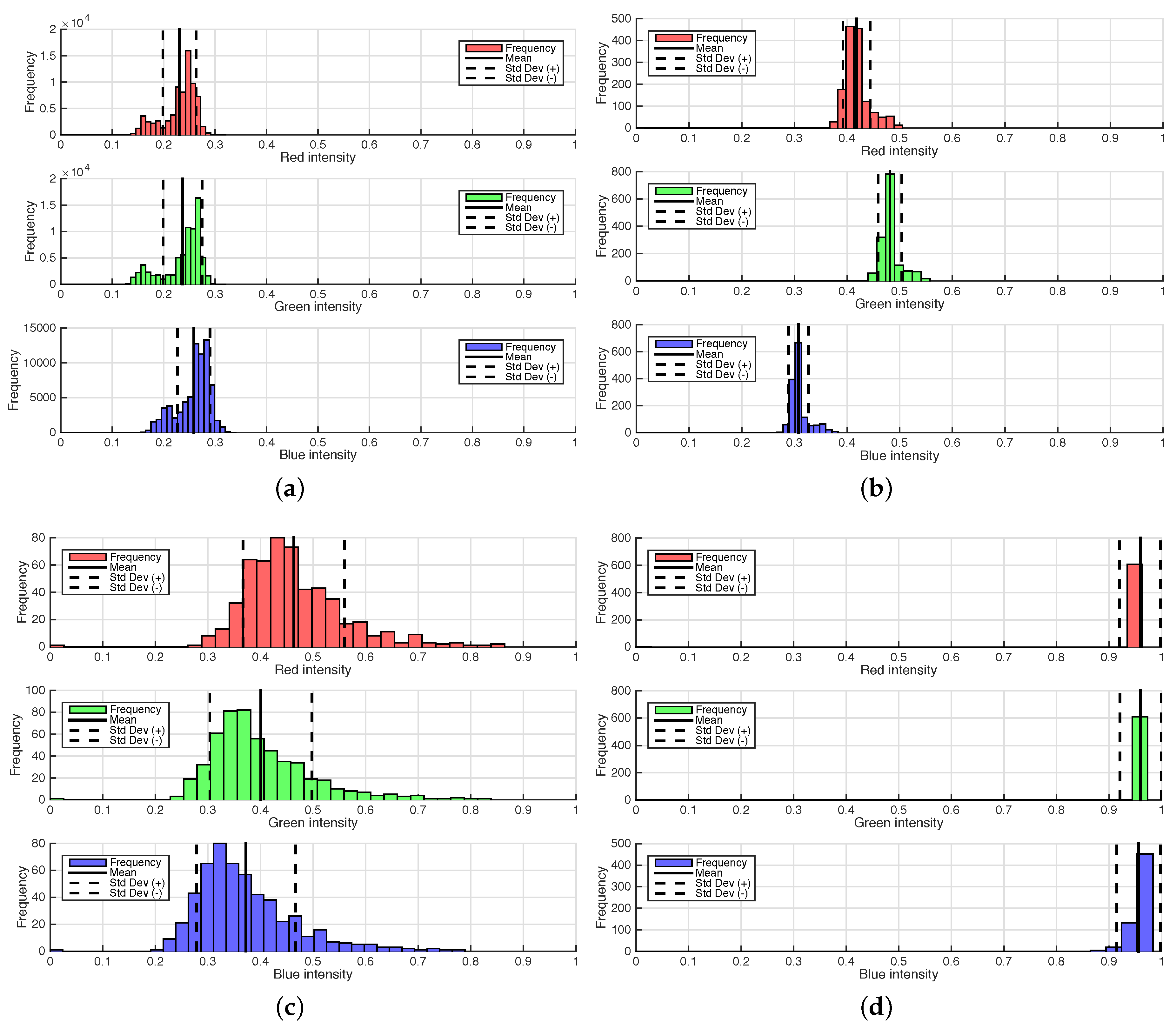
To measure the stalk thickness of a sorghum plant in an image, pixels associated with the stalk must be segmented from pixels associated with other parts of the plant, as well as from the background. K-means clustering and minimum-distance classification were used in this work.

K-Means Algorithm

The K-means clustering algorithm used in this article was adapted from Peter Corke [25] and performs a color-based segmentation based on a pre-selected C number of clusters. The algorithm maps each RGB value to the color xy-chromaticity space and then identifies clusters to segregate the pixels into image classes associated with those clusters. The algorithm initially selects locations in the data space as cluster centers and then calculates the Euclidean distance [26] between each pixel and every cluster center in multiple iterations. At the end of an iteration, each pixel is assigned to the cluster with the closest center, and every cluster center location is recalculated as the average location of the pixels assigned to that cluster. The final result is a classification of the image into C number of classes [25,27,28,29].

Each image was segmented into ten classes. The user identified the five classes that best represented the plants based on whether or not the class clearly contained almost exclusively plant matter, and cluster center locations were stored to a text file. After segmentation, the noise in the image was reduced with a morphological opening with a 9 × 9 square kernel. The five selected classes were then combined to produce a binary image that was an initial separation of plant from background. The combined image was then processed by area opening to remove small artifacts. Finally, to reduce the effects of plant lesions and minor stalk deformities, a morphological closing with a 5 × 5 square kernel was applied to the image. The result was a binary image of the plant segmented from the background; Figure 1a.

Figure 1. RGB original, classified and binary images of sorghum plants during the third week of growth of June, Plant 3B. (a) Segmentation using K-means clustering; (b) segmentation using minimum-distance classification.

Figure 1. RGB original, classified and binary images of sorghum plants during the third week of growth of June, Plant 3B. (a) Segmentation using K-means clustering; (b) segmentation using minimum-distance classification.

Minimum Distance Algorithm

Minimum-distance classification of color images considers the three RGB components as orthogonal coordinates in the Euclidean space, and individual pixels are assigned to classes according to their RGB distance from pixel classes that have been defined by training. Four classes were defined by the user according to homogeneous zones in the images, as shown in Figure 2a. In this figure, the four classes are clearly separable [26]: the black cloth background, enclosed by the blue rectangle; the green sorghum plant leaf, enclosed by the green rectangle; the bright sorghum stalk, enclosed in orange; and the brown soil, enclosed in red. The spectral separability is shown in the histograms of Figure 3. The statistical properties shown are distribution, mean and standard deviation, which were used as the references for the minimum-distance classification algorithm. The mean is the center point to which pixel RGB-space distances are compared, while standard deviation is used as a threshold to determine whether or not a pixel is assigned to a defined class. Each image pixel was compared to all class means, and the shortest distance determined whether a pixel would be assigned to one class or another. A threshold of two standard deviations from all four classes was used to label pixels as “unclassified”. Once the images were processed, the plant regions were stored as binary images (Figure 1b) and used subsequently to calculate stalk thickness.

Figure 2. Images of sorghum Plant 1A on June 30. The minimum distance classification required training samples to segment the images: (a) original image and the location where the samples were obtained, enclosed by rectangles (blue = background; orange = bright stalk; green = plant leaf; red = soil); (b) image segmented into the five classes, including unclassified pixels.

Figure 2. Images of sorghum Plant 1A on June 30. The minimum distance classification required training samples to segment the images: (a) original image and the location where the samples were obtained, enclosed by rectangles (blue = background; orange = bright stalk; green = plant leaf; red = soil); (b) image segmented into the five classes, including unclassified pixels.

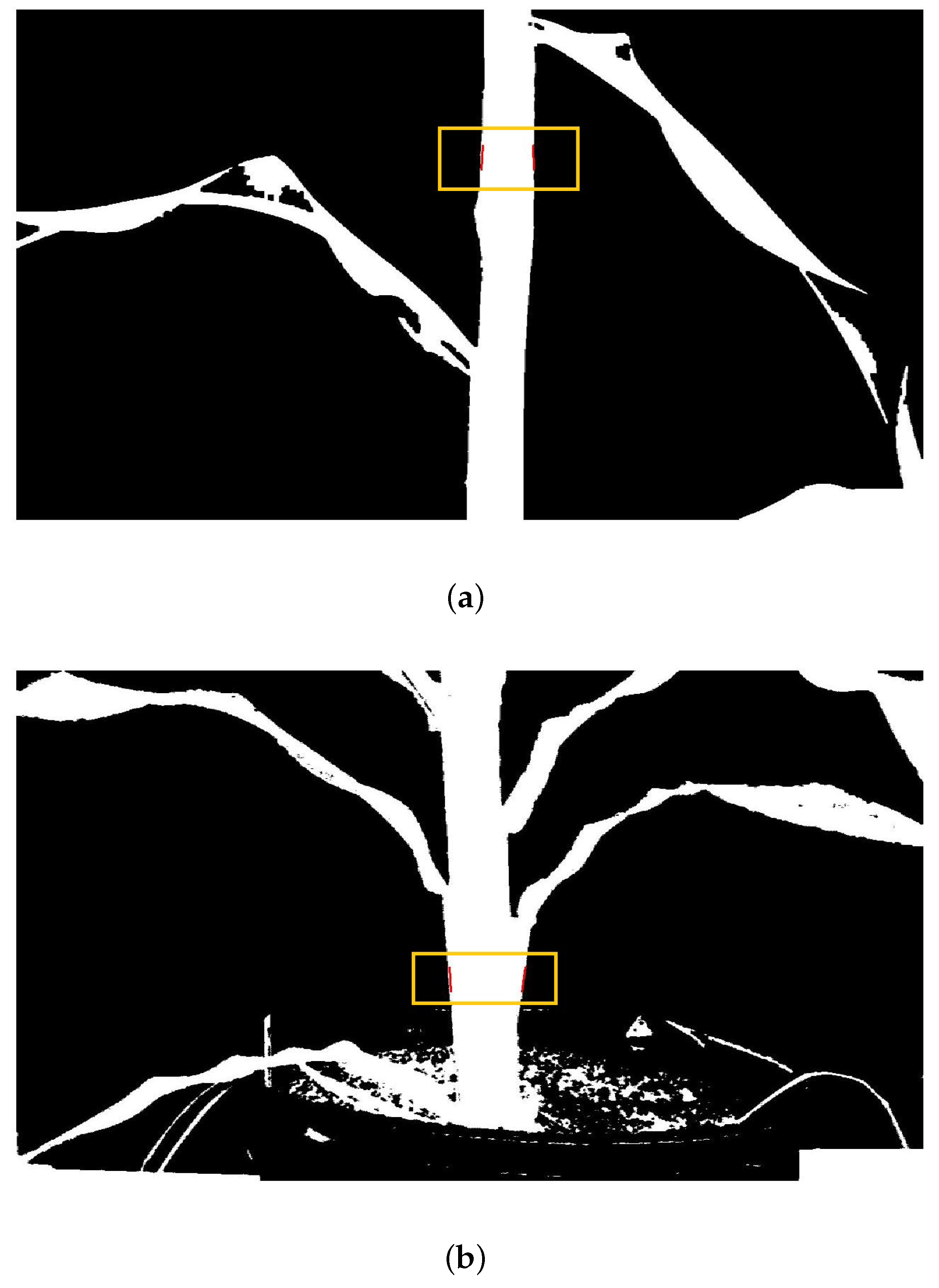
Stalk Thickness Calculation Algorithm

Stalk-thickness calculation was conducted in “supervised” and “unsupervised” modes. In the supervised mode, the user selected a location in the image to define the stalk center. A 3 × 3 pixel window was then used to automatically scan the image in search of the edges of the stalk. Once the edge pixels were identified by the algorithm, stalk thickness in pixels was calculated by subtracting the edge location on the right from the edge location on the left. In unsupervised mode, the user identified the stalk center and allowed the algorithm to select upper and lower stalk thickness measurement locations. The average thickness based on the upper and lower measurements was taken as the stalk thickness (Figure 4). In both modes, stalk thickness in pixels was multiplied by the pixel-length conversion factor, which was dependent on the distance between plant and camera, to obtain stalk thickness in mm.

Figure 3. Frequency histograms of RGB values for each training sample. The solid line in the middle of the distribution indicates the location of the mean value, while the dashed lines indicate the location of two times the standard deviation of the each training sample. The information from the histograms was used to define each class center cluster; meanwhile, the standard deviation was used to define the class threshold. (a) Background; (b) plant; (c) soil; (d) stalk.

Figure 3. Frequency histograms of RGB values for each training sample. The solid line in the middle of the distribution indicates the location of the mean value, while the dashed lines indicate the location of two times the standard deviation of the each training sample. The information from the histograms was used to define each class center cluster; meanwhile, the standard deviation was used to define the class threshold. (a) Background; (b) plant; (c) soil; (d) stalk.

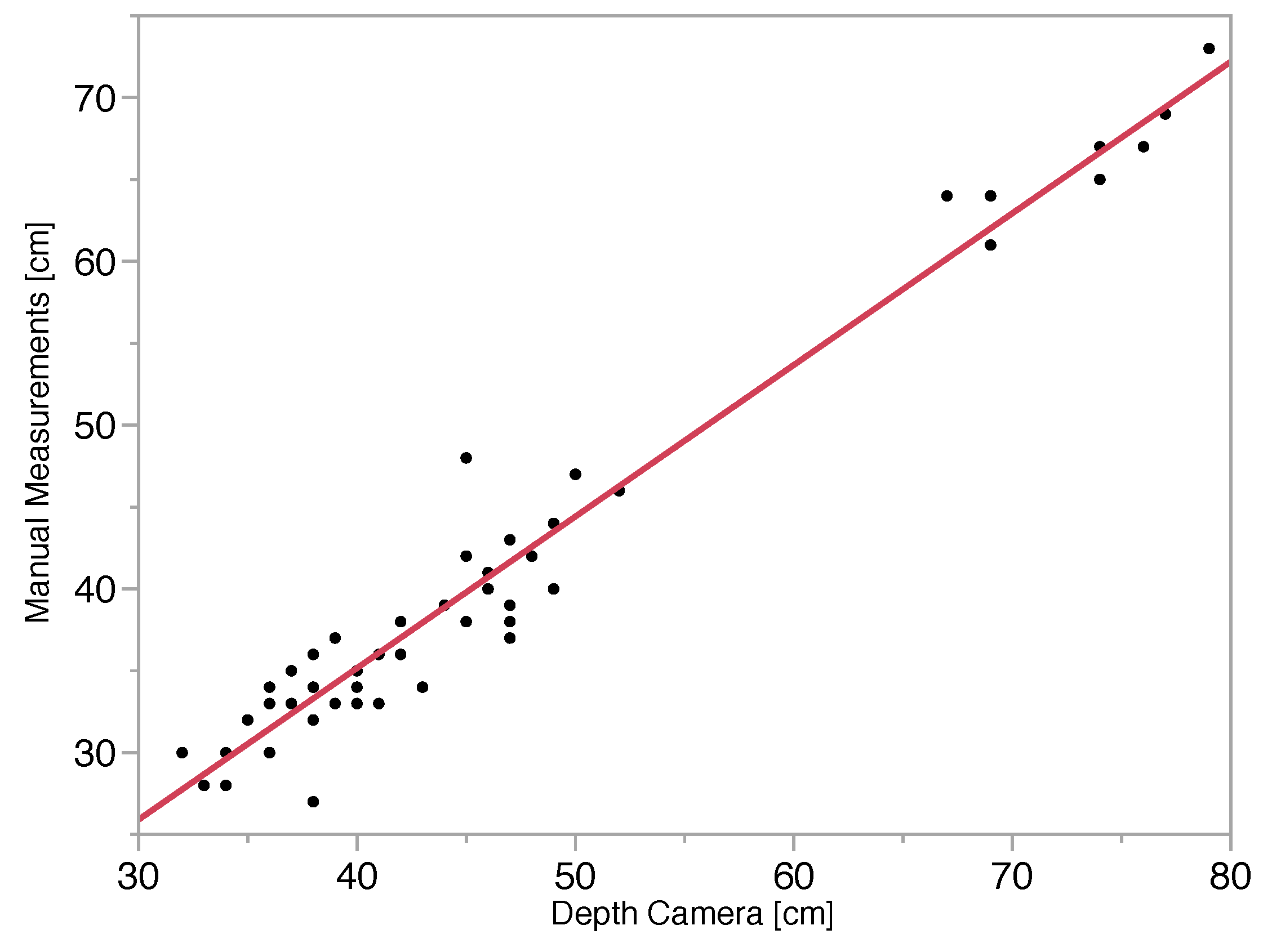
Depth Camera Accuracy

For every plant image collected, a manual measurement of the distance between the camera and plant stalk was conducted with a ruler, to the nearest half centimeter. In the depth-camera images, the pixel values represented the distance between the object and the camera. The depth-camera images included some erroneous pixel values, so the average of a group of pixels belonging to the plant stalk was used to minimize the effect of noise in the images. Two representative areas of the stalk in the depth image were selected by the user, and a 3 × 3 window was selected from each area. The average value from the 18 selected pixels was used as the depth-camera distance between camera and plant. Depth-camera distances were evaluated by comparing them to manual stalk-to-camera distance measurements by way of simple linear regression.

Figure 4. Results of image analysis. The golden box and red lines show the location where the stalk thickness was measured during this procedure: (a) K-means clustering, supervised stalk selection; (b) minimum-distance classification, supervised stalk selection.

Figure 4. Results of image analysis. The golden box and red lines show the location where the stalk thickness was measured during this procedure: (a) K-means clustering, supervised stalk selection; (b) minimum-distance classification, supervised stalk selection.

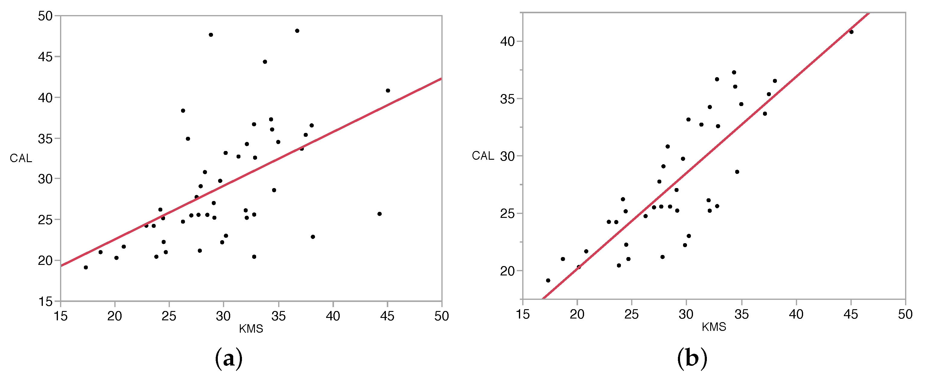
3. Results and Discussion

The stalk thickness values determined through image analysis were compared to the manually-measured values and the percent error calculated for each plant and each date (Table 1). Averaged across all plants and dates, the average percent errors were 27.9 for K-means with unsupervised stalk measurement (KMU), 19.5 for minimum distance with unsupervised stalk measurement (MDU), 16.0 for K-means with supervised stalk measurement (KMS) and 16.7 for minimum distance with supervised stalk measurement (MDS). All KMS stalk-thickness measurements are plotted against the caliper values in Figure 5a. Linear regression of these data points resulted in an R² value of 0.28, indicating that KMS measurements only account for 28% of the variability in the caliper measurements.

Table 1. Comparison of stalk thickness measurements using K-means unsupervised (KMU), K-means supervised (KMS), minimum-distance unsupervised (MDU) and minimum-distance supervised (MDS) modes. The plant ID shows the plant number and the variety. The measured value indicates the value obtained with the stalk thickness calculation algorithm. The points in bold were determined to be outliers and removed from the final analysis (see Figure 5).

			Measured Value (mm)				Percent Error (%)
Date	Plant ID	Caliper Reading (mm)	KMU	MDU	KMS	MDS	KMU	MDU	KMS	MDS
30 June	1A	25.58	24.12	32.27	28.47	27.47	5.71	26.17	11.29	7.41
	2A	33.17	28.96	40.13	30.15	29.18	12.69	20.98	9.12	12.04
	3A	30.82	31.18	31.41	28.25	26.88	1.17	1.91	8.32	12.77
	4A	32.59	35.75	35.11	32.85	27.31	9.70	7.74	0.80	16.20
	1B	29.75	21.84	30.62	29.65	31.45	26.59	2.92	0.35	5.70
	2B	28.61	27.57	37.41	34.60	32.96	3.64	30.78	20.95	15.19
	3B	27.76	21.65	26.22	27.49	25.36	22.01	5.56	0.96	8.65
	4B	25.62	60.49	39.14	32.77	26.98	136.10	52.79	27.90	5.29
7 July	1A	40.81	19.07	58.85	45.05	49.09	53.27	44.20	10.38	20.28
	2A	48.14	34.41	41.70	36.72	38.83	28.52	13.38	23.73	19.34
	3A	34.91	20.73	35.05	26.69	26.85	40.62	0.40	23.55	23.08
	4A	44.34	29.50	36.88	33.76	34.52	33.47	16.82	23.86	22.15
	1B	38.35	15.44	31.84	26.24	29.48	59.74	16.97	31.58	23.13
	2B	32.73	21.52	32.23	31.33	29.43	34.25	1.51	4.29	10.07
	3B	29.09	25.07	30.90	27.86	30.43	13.82	6.22	4.23	4.61
	4B	47.65	20.16	28.48	28.80	29.31	57.69	40.23	39.56	38.49
14 July	1A	36.54	35.44	34.25	38.05	32.10	3.01	6.27	4.13	12.16
	2A	36.04	40.80	40.50	34.42	32.92	13.21	12.38	4.51	8.64
	3A	35.38	41.10	41.98	37.50	36.87	16.17	18.65	5.99	4.22
	4A	33.68	41.59	35.09	37.14	36.47	23.49	4.20	10.27	8.29
	1B	36.68	35.40	36.81	32.76	31.55	3.49	0.37	10.69	14.00
	2B	34.51	31.20	36.08	34.98	35.55	9.59	4.54	1.36	3.00
	3B	22.22	35.39	38.57	29.83	30.71	59.27	73.59	34.23	38.23
	4B	37.28	44.04	34.63	34.32	31.37	18.13	7.11	7.94	15.85
21 July	1A	20.45	28.60	31.55	32.77	31.88	39.85	54.29	60.24	55.91
	2A	25.51	22.77	25.98	27.00	26.77	10.74	1.84	5.82	4.94
	3A	25.17	24.36	26.34	24.41	24.77	3.22	4.65	3.04	1.59
	4A	34.26	31.41	32.74	32.10	32.20	8.32	4.43	6.32	6.01
	1B	21.01	16.10	57.74	18.67	17.11	23.37	174.81	11.16	18.58
	2B	24.75	37.99	25.20	26.23	27.25	53.49	1.83	5.98	10.11
	3B	25.70	43.96	39.39	44.28	44.75	71.05	53.28	72.30	74.13
	4B	22.89	37.24	36.41	38.16	38.99	62.69	59.07	66.71	70.32
4 August	1A	21.01	24.12	23.31	24.66	23.14	14.80	10.97	17.35	10.12
	2A	25.22	28.96	29.13	32.09	32.09	14.83	15.50	27.24	27.24
	3A	25.58	31.18	26.33	27.66	26.99	21.89	2.94	8.13	5.51
	4A	27.03	35.75	24.83	29.06	29.70	32.26	8.15	7.49	9.88
	1B	20.45	21.84	21.55	23.79	23.54	6.80	5.39	16.31	15.11
	2B	23.02	27.57	27.43	30.18	30.48	19.77	19.17	31.08	32.41
	3B	22.26	21.65	21.28	24.46	25.90	2.74	4.42	9.88	16.33
	4B	26.22	60.49	22.49	24.16	24.31	130.70	14.21	7.88	7.29
11 August	1A	24.23	19.07	23.31	23.55	23.64	21.30	3.78	2.83	2.42
	2A	25.23	34.41	29.13	29.12	27.96	36.39	15.46	15.42	10.81
	3A	24.25	20.73	26.33	22.87	21.86	14.52	8.59	5.69	9.86
	4A	26.13	29.50	24.83	31.99	30.26	12.90	4.99	22.43	15.80
	1B	19.14	15.44	21.55	17.32	17.40	19.33	12.60	9.51	9.07
	2B	20.31	21.52	27.43	20.13	20.32	5.96	35.07	0.91	0.02
	3B	21.19	25.07	21.28	27.78	28.26	18.31	0.41	31.08	33.38
	4B	21.68	20.16	22.49	20.80	20.96	7.01	3.76	4.06	3.34

Table 1. Comparison of stalk thickness measurements using K-means unsupervised (KMU), K-means supervised (KMS), minimum-distance unsupervised (MDU) and minimum-distance supervised (MDS) modes. The plant ID shows the plant number and the variety. The measured value indicates the value obtained with the stalk thickness calculation algorithm. The points in bold were determined to be outliers and removed from the final analysis (see Figure 5).

			Measured Value (mm)				Percent Error (%)
Date	Plant ID	Caliper Reading (mm)	KMU	MDU	KMS	MDS	KMU	MDU	KMS	MDS
30 June	1A	25.58	24.12	32.27	28.47	27.47	5.71	26.17	11.29	7.41
	2A	33.17	28.96	40.13	30.15	29.18	12.69	20.98	9.12	12.04
	3A	30.82	31.18	31.41	28.25	26.88	1.17	1.91	8.32	12.77
	4A	32.59	35.75	35.11	32.85	27.31	9.70	7.74	0.80	16.20
	1B	29.75	21.84	30.62	29.65	31.45	26.59	2.92	0.35	5.70
	2B	28.61	27.57	37.41	34.60	32.96	3.64	30.78	20.95	15.19
	3B	27.76	21.65	26.22	27.49	25.36	22.01	5.56	0.96	8.65
	4B	25.62	60.49	39.14	32.77	26.98	136.10	52.79	27.90	5.29
7 July	1A	40.81	19.07	58.85	45.05	49.09	53.27	44.20	10.38	20.28
	2A	48.14	34.41	41.70	36.72	38.83	28.52	13.38	23.73	19.34
	3A	34.91	20.73	35.05	26.69	26.85	40.62	0.40	23.55	23.08
	4A	44.34	29.50	36.88	33.76	34.52	33.47	16.82	23.86	22.15
	1B	38.35	15.44	31.84	26.24	29.48	59.74	16.97	31.58	23.13
	2B	32.73	21.52	32.23	31.33	29.43	34.25	1.51	4.29	10.07
	3B	29.09	25.07	30.90	27.86	30.43	13.82	6.22	4.23	4.61
	4B	47.65	20.16	28.48	28.80	29.31	57.69	40.23	39.56	38.49
14 July	1A	36.54	35.44	34.25	38.05	32.10	3.01	6.27	4.13	12.16
	2A	36.04	40.80	40.50	34.42	32.92	13.21	12.38	4.51	8.64
	3A	35.38	41.10	41.98	37.50	36.87	16.17	18.65	5.99	4.22
	4A	33.68	41.59	35.09	37.14	36.47	23.49	4.20	10.27	8.29
	1B	36.68	35.40	36.81	32.76	31.55	3.49	0.37	10.69	14.00
	2B	34.51	31.20	36.08	34.98	35.55	9.59	4.54	1.36	3.00
	3B	22.22	35.39	38.57	29.83	30.71	59.27	73.59	34.23	38.23
	4B	37.28	44.04	34.63	34.32	31.37	18.13	7.11	7.94	15.85
21 July	1A	20.45	28.60	31.55	32.77	31.88	39.85	54.29	60.24	55.91
	2A	25.51	22.77	25.98	27.00	26.77	10.74	1.84	5.82	4.94
	3A	25.17	24.36	26.34	24.41	24.77	3.22	4.65	3.04	1.59
	4A	34.26	31.41	32.74	32.10	32.20	8.32	4.43	6.32	6.01
	1B	21.01	16.10	57.74	18.67	17.11	23.37	174.81	11.16	18.58
	2B	24.75	37.99	25.20	26.23	27.25	53.49	1.83	5.98	10.11
	3B	25.70	43.96	39.39	44.28	44.75	71.05	53.28	72.30	74.13
	4B	22.89	37.24	36.41	38.16	38.99	62.69	59.07	66.71	70.32
4 August	1A	21.01	24.12	23.31	24.66	23.14	14.80	10.97	17.35	10.12
	2A	25.22	28.96	29.13	32.09	32.09	14.83	15.50	27.24	27.24
	3A	25.58	31.18	26.33	27.66	26.99	21.89	2.94	8.13	5.51
	4A	27.03	35.75	24.83	29.06	29.70	32.26	8.15	7.49	9.88
	1B	20.45	21.84	21.55	23.79	23.54	6.80	5.39	16.31	15.11
	2B	23.02	27.57	27.43	30.18	30.48	19.77	19.17	31.08	32.41
	3B	22.26	21.65	21.28	24.46	25.90	2.74	4.42	9.88	16.33
	4B	26.22	60.49	22.49	24.16	24.31	130.70	14.21	7.88	7.29
11 August	1A	24.23	19.07	23.31	23.55	23.64	21.30	3.78	2.83	2.42
	2A	25.23	34.41	29.13	29.12	27.96	36.39	15.46	15.42	10.81
	3A	24.25	20.73	26.33	22.87	21.86	14.52	8.59	5.69	9.86
	4A	26.13	29.50	24.83	31.99	30.26	12.90	4.99	22.43	15.80
	1B	19.14	15.44	21.55	17.32	17.40	19.33	12.60	9.51	9.07
	2B	20.31	21.52	27.43	20.13	20.32	5.96	35.07	0.91	0.02
	3B	21.19	25.07	21.28	27.78	28.26	18.31	0.41	31.08	33.38
	4B	21.68	20.16	22.49	20.80	20.96	7.01	3.76	4.06	3.34

Close inspection of Figure 5a indicated that several of the data points may be outliers, so the following procedure (adapted from [30,31]) was used in an effort to identify actual outliers that should be removed from consideration. (1) Residuals were calculated and plotted against the caliper measurements, indicating heteroscedasticity (i.e., residual values were lower at low stalk thickness values and higher at high stalk thickness values). (2) Based on the fact that residuals were heteroscedastic, both KMS and caliper measurements were transformed by taking their logarithms. Log(caliper) was regressed against log(KMS), and residuals were again plotted, indicating that heteroscedasticity had been mitigated. (3) Studentized residuals of the log(caliper) vs. log(KMS) relationship were calculated, and the distribution of the studentized residuals was determined. At the positive and negative tails of the distribution, seven data points were identified as being significantly disconnected from the rest of the data. This evaluation provided the basis for identifying suspected possible outliers. (4) The original images associated with the suspected outliers were observed to determine whether anomalies that could produce major errors could be identified. With each of the suspected outliers, the images suggested that significant error-causing anomalies were present, so these data points were removed, and simple linear regression was conducted on the resulting dataset (Figure 5b). Results of the analysis after removing outliers provided an R² value of 0.70, indicating that KMS measurements accounted for 70% of the variability in the caliper measurements. Furthermore, with the outliers (identified in Table 1) removed, the resulting average error for KMS measurements was reduced to 10.7%.

Figure 5. Linear regressions for caliper measurements vs. K-means supervised measurements: (a) the regression before removing outliers (R² = 0.28, RMSE 6.27 mm); (b) after removal of outliers (R² = 0.70, RMSE 3.19 mm). Plot units are in mm.

Figure 5. Linear regressions for caliper measurements vs. K-means supervised measurements: (a) the regression before removing outliers (R² = 0.28, RMSE 6.27 mm); (b) after removal of outliers (R² = 0.70, RMSE 3.19 mm). Plot units are in mm.

As a representation of the image classification errors, Figure 6 shows the original and two classified images of Plant 4B on 30 June, which had the highest error of all plants measured on that date (except with MDS). It can be observed that this plant had leaves emerging from the sides of the stalk over most of the stalk area. This problem made it difficult for the stalk measurement algorithm to identify the actual edges of the stalk, contributing error to the measurement. On 7 July, the plant with the highest percent error had non-plant pixels in the binary image of the stalk, indicating poor segmentation that led the analysis to measure only part of the stalk. These are the types of errors common to the high error image-based measurements.

Figure 6. The images presented are examples of anomalies in the experiment. K-means, unsupervised (KMU), minimum-distance, unsupervised (MDU) and K-means, supervised (KMS) were three out of the four different methods in this experiment. (a) 30 June, 4B; (b) 30 June, 4B, KMU (136.10); (c) 30 June, 4B, MDU (52.79). In parenthesis, the error between the manual measurement and algorithm measurement is shown (see also Table 1).

Figure 6. The images presented are examples of anomalies in the experiment. K-means, unsupervised (KMU), minimum-distance, unsupervised (MDU) and K-means, supervised (KMS) were three out of the four different methods in this experiment. (a) 30 June, 4B; (b) 30 June, 4B, KMU (136.10); (c) 30 June, 4B, MDU (52.79). In parenthesis, the error between the manual measurement and algorithm measurement is shown (see also Table 1).

In terms of the plant growth stage at which measurements were most accurate, later-stage plants had lower error than early-stage plants. By the seven-week point, the plants had developed reasonably well-defined stalks that were easier to segment and measure. The relatively low percent error at later growth stages showed the techniques to be most accurate at the time phenotyping would be most useful. In terms of which methods were most accurate, K-means clustering was more accurate with supervised stalk measurement, but minimum-distance classification was more accurate with unsupervised stalk measurement. Supervised stalk measurement had lower error than unsupervised when using either K-means or minimum distance. This result suggests that the position where stalk thickness is measured is critical to the accuracy of the measurement, and future research should focus on how the image-processing algorithm determines the best measurement location. As previously mentioned, the most obvious errors in measuring stalk thickness occurred when leaves protruding from the stalk were included in the stalk-thickness measurement. Additional image-processing techniques—e.g., to consider whether the left and right stalk edges are parallel—could better isolate the stalk, enabling the largest stalk thickness measurement errors to be mitigated. In other cases, the source of major error was either unknown or related to poor image segmentation, probably due to lack of contrast at particular points on the plant. To mitigate these errors, more research would be required, as solutions are not obvious.

The results of comparing depth-camera distance measurements to manual camera-to-stalk distance measurements are presented in Figure 7. The plot of data points indicates a high level of linearity, and the R² value of 0.96 indicates that the depth camera accounted for 96% of the variability in actual camera-to-stalk distance. The average error for camera-to-stalk distance on a given day ranged from about 5% to 20%, while the root mean square error (RMSE) was 2.5 cm. It is clear from the plot that at camera-to stalk distances greater than 65 cm, the percent error is low. Stalk thickness error associated with a depth-camera distance RMSE of 2.5 cm is approximately 3%, meaning that the roughly 10% average stalk thickness error resulting from image processing is large compared to depth-camera error. The depth-camera feature of this combined camera thus appears to be acceptably accurate to provide distance data that would enable calculation of pixel-to-length conversion factors. If this capability could be combined with the image-processing techniques to segment the plant and calculate the number of pixels associated with the thickness of a stalk, then stalk thickness measurement for energy sorghum plants could be fully automated. The issue of pixel-to-pixel correspondence between depth images and RGB images is an issue remaining to be solved.

Figure 7. Linear regression of distance measurements from the camera to the plant, measured manually and measured with the depth camera images. The R² value calculated for this relationship is 0.96, and the RMSE is 2.5 cm.

Figure 7. Linear regression of distance measurements from the camera to the plant, measured manually and measured with the depth camera images. The R² value calculated for this relationship is 0.96, and the RMSE is 2.5 cm.

4. Conclusions

This study showed that an inexpensive combined (RGB plus depth) camera and common image analysis techniques (K-means clustering and minimum-distance classification) have potential for measuring stalk thickness in a high-throughput phenotyping system for energy sorghum plants. Furthermore, the integrated near-infrared time-of-flight depth camera showed excellent potential for providing distance measurements that would be required if stalk thickness were to be measured in an automated way. Incidentally, these techniques could be applied to other monocots, such as maize and rice. If successfully implemented, such a combined system could greatly reduce the labor and time required to make such measurements in experiments involving phenotyping, ultimately enabling many more plants to be measured than currently possible and potentially accelerating crop improvement.

References

1. Davies, J. Better distribution holds the key to future food security for all. Poult. World 2015, 170, 1–19. [Google Scholar]
2. Koçar, G.; Civas, N. An overview of biofuels from energy crops: Current status and future prospects. Renew. Sustain. Energy Rev. 2013, 28, 900–916. [Google Scholar] [CrossRef]
3. Chapman, S.C.; Chakraborty, S.; Dreccer, M.F.; Howden, S.M. Plant adaptation to climate change—Opportunities and priorities in breeding. Crop Pasture Sci. 2012, 63, 251–268. [Google Scholar] [CrossRef]
4. Calviño, M.; Messing, J. Sweet sorghum as a model system for bioenergy crops. Curr. Opin. Biotechnol. 2012, 23, 323–329. [Google Scholar] [CrossRef] [PubMed]
5. Cobb, J.N.; DeClerck, G.; Greenberg, A.; Clark, R.; McCouch, S. Next-generation phenotyping: Requirements and strategies for enhancing our understanding of genotype–phenotype relationships and its relevance to crop improvement. Theor. Appl. Genet. 2013, 126, 867–887. [Google Scholar] [CrossRef] [PubMed]
6. Regassa, T.H.; Wortmann, C.S. Sweet sorghum as a bioenergy crop: Literature review. Biomass Bioenergy 2014, 64, 348–355. [Google Scholar] [CrossRef]
7. Busemeyer, L.; Mentrup, D.; Möller, K.; Wunder, E.; Alheit, K.; Hahn, V.; Maurer, H.P.; Reif, J.C.; Würschum, T.; Müller, J.; et al. BreedVision—A Multi-Sensor Platform for Non-Destructive Field-Based Phenotyping in Plant Breeding. Sensors 2013, 13, 2830–2847. [Google Scholar] [CrossRef] [PubMed]
8. Kicherer, A.; Herzog, K.; Pflanz, M.; Wieland, M.; Rüger, P.; Kecke, S.; Kuhlmann, H.; Töpfer, R. An Automated Field Phenotyping Pipeline for Application in Grapevine Research. Sensors 2015, 15, 4823–4836. [Google Scholar] [CrossRef] [PubMed]
9. Klodt, M.; Herzog, K.; Töpfer, R.; Cremers, D. Field phenotyping of grapevine growth using dense stereo reconstruction. BMC Bioinf. 2015, 16, 1–11. [Google Scholar] [CrossRef] [PubMed]
10. Upadhyaya, H.; Wang, Y.H.; Sharma, S.; Singh, S.; Hasenstein, K. SSR markers linked to kernel weight and tiller number in sorghum identified by association mapping. Euphytica 2012, 187, 401–410. [Google Scholar] [CrossRef] [Green Version]
11. Mullet, J.; Morishige, D.; McCormick, R.; Truong, S.; Hilley, J.; McKinley, B.; Anderson, R.; Olson, S.; Rooney, W. Energy Sorghum—A genetic model for the design of C4 grass bioenergy crops. J. Exp. Bot. 2014, 65, 1–11. [Google Scholar] [CrossRef] [PubMed]
12. van der Weijde, T.; Alvim Kamei, C.L.; Torres, A.F.; Wilfred, V.; Oene, D.; Visser, R.G.F.; Trindade, L.M. The potential of C4 grasses for cellulosic biofuel production. Front. Plant Sci. 2013, 4, 1–18. [Google Scholar] [CrossRef] [PubMed]
13. Trouche, G.; Bastianelli, D.; Cao Hamadou, T.V.; Chantereau, J.; Rami, J.F.; Pot, D. Exploring the variability of a photoperiod-insensitive sorghum genetic panel for stem composition and related traits in temperate environments. Field Crops Res. 2014, 166, 72–81. [Google Scholar] [CrossRef]
14. Chéné, Y.; Rousseau, D.; Lucidarme, P.; Bertheloot, J.; Caffier, V.; Morel, P.; Belin, É.; Chapeau-Blondeau, F. On the use of depth camera for 3D phenotyping of entire plants. Comput. Electron. Agric. 2012, 82, 122–127. [Google Scholar] [CrossRef] [Green Version]
15. Vollmann, J.; Walter, H.; Sato, T.; Schweiger, P. Digital image analysis and chlorophyll metering for phenotyping the effects of nodulation in soybean. Comput. Electron. Agric. 2011, 75, 190–195. [Google Scholar] [CrossRef]
16. Chaivivatrakul, S.; Tang, L.; Dailey, M.N.; Nakarmi, A.D. Automatic morphological trait characterization for corn plants via 3D holographic reconstruction. Comput. Electron. Agric. 2014, 109, 109–123. [Google Scholar] [CrossRef]
17. Roscher, R.; Herzog, K.; Kunkel, A.; Kicherer, A.; Töpfer, R.; Förstner, W. Automated image analysis framework for high-throughput determination of grapevine berry sizes using conditional random fields. Comput. Electron. Agric. 2014, 100, 148–158. [Google Scholar] [CrossRef]
18. Aksoy, E.E.; Abramov, A.; Wörgötter, F.; Scharr, H.; Fischbach, A.; Dellen, B. Modeling leaf growth of rosette plants using infrared stereo image sequences. Comput. Electron. Agric. 2015, 110, 78–90. [Google Scholar] [CrossRef]
19. Fahlgren, N.; Gehan, M.A.; Baxter, I. Lights, camera, action: High-throughput plant phenotyping is ready for a close-up. Curr. Opin. Plant Biol. 2015, 24, 93–99. [Google Scholar] [CrossRef] [PubMed]
20. Kolukisaoglu, Ü.; Thurow, K. Future and frontiers of automated screening in plant sciences. Plant Sci. 2010, 178, 476–484. [Google Scholar] [CrossRef]
21. Lobet, G.; Draye, X.; Périlleux, C. An online database for plant image analysis software tools. Plant Methods 2013, 9. [Google Scholar] [CrossRef] [PubMed]
22. Colombi, T.; Kirchgessner, N.; Le Marié, C.; York, L.; Lynch, J.; Hund, A. Next generation shovelomics: Set up a tent and REST. Plant Soil 2015, 388, 1–20. [Google Scholar] [CrossRef]
23. Bucksch, A.; Burridge, J.; York, L.M.; Das, A.; Nord, E.; Weitz, J.S.; Lynch, J. Image-Based High-Throughput Field Phenotyping of Crop Roots. Plant Physiol. 2014, 166, 470–486. [Google Scholar] [CrossRef] [PubMed]
24. Rooney, W.L.; (Soil and Crop Science Professor, Texas A&M University, College Station, TX, USA) Stalk diameter measure location in energy sorghum. Personal communication, 2015.
25. Corke, P. Robotics, Vision and Control: Fundamental Algorithms in MATLAB; Springer Science & Business Media: Berlin, Germany, 2011; Volume 73. [Google Scholar]
26. Ghimire, S.; Wang, H. Classification of image pixels based on minimum distance and hypothesis testing. Comput. Stat. Data Anal. 2012, 56, 2273–2287. [Google Scholar] [CrossRef]
27. Liang, B.; Zhang, J. KmsGC: An Unsupervised Color Image Segmentation Algorithm Based on K-Means Clustering and Graph Cut. Math. Probl. Eng. 2014, 2014, 464875. [Google Scholar] [CrossRef]
28. Sert, E.; Okumus, I.T. Segmentation of mushroom and cap width measurement using modified K-means clustering algorithm. Adv. Electr. Electron. Eng. 2014, 12, 354–360. [Google Scholar] [CrossRef]
29. Yu, W.; Wang, J.; Ye, L. An Improved Normalized Cut Image Segmentation Algorithm with K-means Cluster. Appl. Mech. Mater. 2014, 548–549, 1179–1184. [Google Scholar] [CrossRef]
30. Neter, J.; Kutner, M.H.; Nachtsheim, C.J.; Wasserman, W. Applied Linear Statistical Models, 4th ed.; McGraw-Hill: Boston, MA, USA, 1996. [Google Scholar]
31. Cline, D. Statistical Analysis; STAT 601 Class Notes; Texas A&M University: College Station, TX, USA, 2015. [Google Scholar]