Optimized Distributed Hyperparameter Search and Simulation for Lung Texture Classification in CT Using Hadoop

Abstract

Many medical image analysis tasks require complex learning strategies to reach a quality of image-based decision support that is sufficient in clinical practice. The analysis of medical texture in tomographic images, for example of lung tissue, is no exception. Via a learning framework, very good classification accuracy can be obtained, but several parameters need to be optimized. This article describes a practical framework for efficient distributed parameter optimization. The proposed solutions are applicable for many research groups with heterogeneous computing infrastructures and for various machine learning algorithms. These infrastructures can easily be connected via distributed computation frameworks. We use the Hadoop framework to run and distribute both grid and random search strategies for hyperparameter optimization and cross-validations on a cluster of 21 nodes composed of desktop computers and servers. We show that significant speedups of up to 364× compared to a serial execution can be achieved using our in-house Hadoop cluster by distributing the computation and automatically pruning the search space while still identifying the best-performing parameter combinations. To the best of our knowledge, this is the first article presenting practical results in detail for complex data analysis tasks on such a heterogeneous infrastructure together with a linked simulation framework that allows for computing resource planning. The results are directly applicable in many scenarios and allow implementing an efficient and effective strategy for medical (image) data analysis and related learning approaches.

1. Introduction

Exhaustive grid parameter search is a widely-used hyperparameter optimization strategy in the context of machine learning [1]. Typically, it is used to search through a manually-defined subset of hyperparameters of a learning algorithm. It is a simple tool for optimizing the performance of machine learning algorithms and can explore all regions of the defined search space if no local extrema exist, and the surfaces of the parameter combinations are relatively smooth. However, it involves high computational costs, increasing exponentially with the number of hyperparameters, as one predictive model needs to be constructed for each combination of parameters (and possibly for each fold of a Cross–Validation (CV)). It can therefore be extremely time-consuming (taking multiple days, weeks or even months of computation depending on the infrastructure available) even for learning algorithms with a small number of hyperparameters, which is often the case. Random search is another approach that randomly samples parameters in a defined search space. It can also be very time-consuming when working with a large number of hyperparameters and a large number of sample points in the search space. Random search can be more suited if highly local optimal parameter combinations exist that might be missed with grid search. It is a less reproducible approach though. Fortunately, grid, random and similar parameter search paradigms are typically “embarrassingly parallel” (https://en.wikipedia.org/wiki/Embarrassingly_parallel, as of 18 February 2016) problems, as the computation required for building the predictive model for an individual parameter setting does not depend on the others [2].

Distributed computing frameworks can help with saving time by running independent tasks simultaneously on multiple computers [3], including local hardware resources, as well as cloud computing resources. These frameworks can use Central Processing Units (CPUs), Graphical Processing Units (GPUs) (which have received much attention recently, especially in the field of deep learning) or a combination of both. Various paradigms for distributed computing exist: Message Passing Interface (MPI) (https://en.wikipedia.org/wiki/Message_Passing_Interface, as of 18 February 2016) and related projects, such as Open Multi–Processing (OpenMP) are geared towards shared memory and efficient multi-threading. They are well-suited for large computational problems requiring frequent communication between threads (either on a single computer or over a network) and are classically targeted at languages, such as C, C++ or Fortran. They offer fast performance, but can increase the complexity of software development and require high-performance networking in order to avoid bottlenecks when working with large amounts of data. Other paradigms for large-scale data processing, including MapReduce implementations, such as Apache Hadoop (http://hadoop.apache.org/, as of 18 February 2016), are more aimed towards data locality, fault tolerance, commodity hardware and simple programming (with a stronger link to languages, such as Java or Python). They are more suited for the parallelization of general computation or data processing tasks, with specific tools available for different kinds of processing (for example, Apache Spark (http://spark.apache.org/, as of 18 February 2016) for in-memory processing or Apache Storm (http://storm.apache.org/, as of 18 February 2016) for real-time stream-based computation). All of these frameworks are commonly used in medical imaging and machine learning research [3,4].

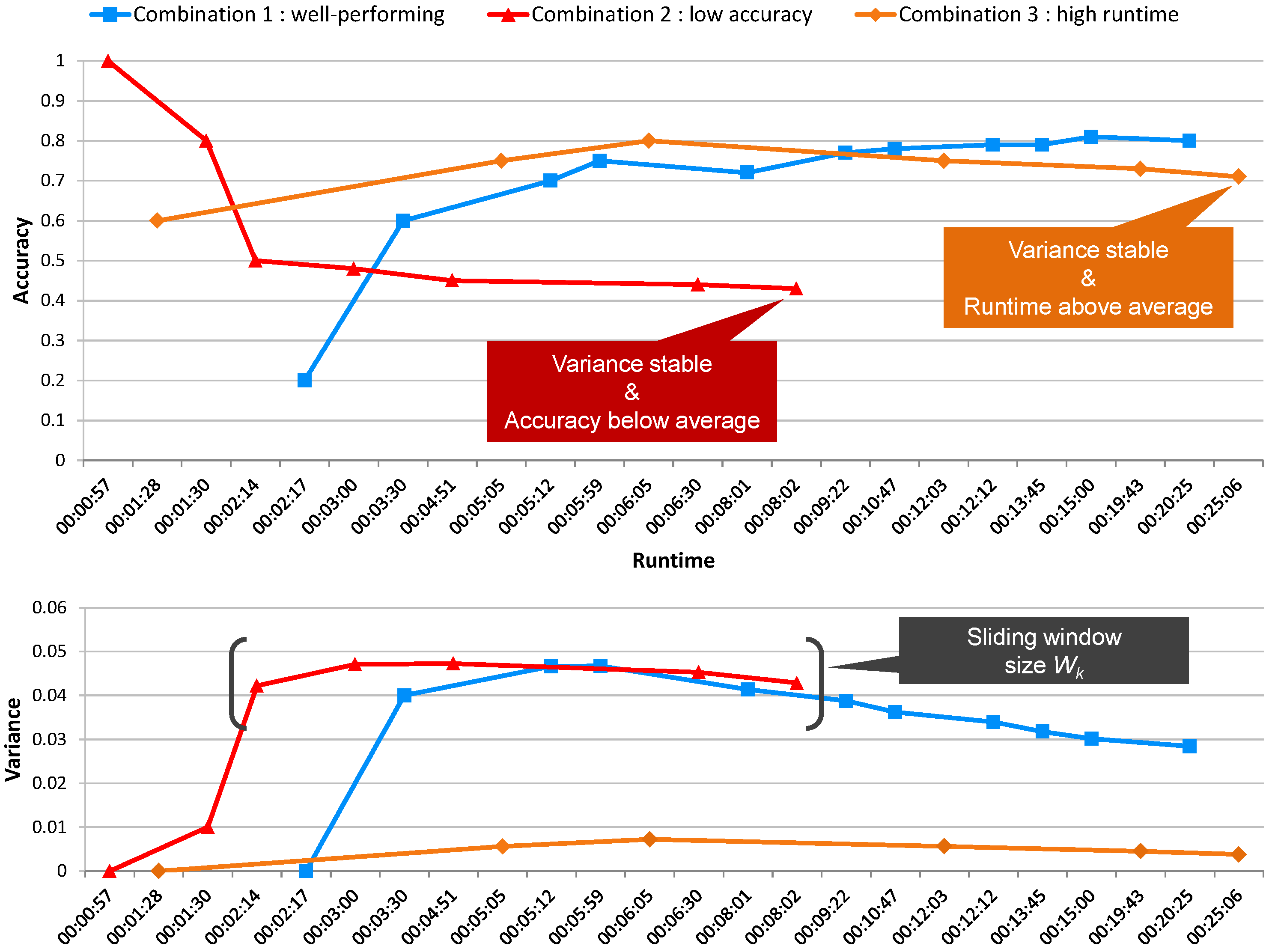
It is also noteworthy to mention that although hyperparameter search should be as exhaustive as possible, there often exist large areas of the search domain that produce suboptimal results, therefore offering opportunities to intelligently reduce the search space and computation time. In a distributed setting, this can complicate the process, as the pruning operation requires sharing information between tasks. To this end, a distributed synchronization mechanism can be designed to allow identifying parameter combinations yielding suboptimal results and subsequently canceling their execution in order to further decrease the total computational time. Moreover, parameter search can be a lengthy process, even when executed within a distributed environment. Therefore, the availability of a parallel execution simulation tool can help estimate the total runtime for varying conditions, such as the number of available computation tasks. Such a simulation tool can also be useful for price estimation when using “pay-as-you-go” computing resources in the cloud (most cloud providers offer specific Hadoop instance types and simple cluster setup tools). This allows making a trade-off between the expected optimization of parameters vs. the related costs.

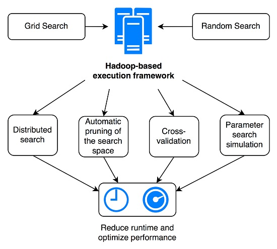
In this article, we present a novel practical framework for the simulation, optimization and execution of parallel parameter search for machine learning algorithms in the context of medical image analysis. It combines all of the aspects discussed above: (i) parallel execution of parameter search, (ii) intelligent identification and cancellation of suboptimal parameter combinations within the distributed environment and (iii) simulation of the total parallel runtime according to the number of computing nodes available when executed in a distributed architecture. The objective is to allow easily running very fine-grained grid or random parameter search experiments in a reasonable amount of time, while maximizing the likelihood of finding one of the best-performing parameter combinations. We evaluated our framework with two use-cases in the article: lung tissue identification in Computed Tomography (CT) images using (I) Support Vector Machines (SVMs) based on a Radial Basis Function (RBF) kernel and (II) Random Forests (RFs). Results for both grid and random search strategies are provided. The main contributions of the article concern the practical design, implementation and testing of a distributed parameter optimization framework, leveraging software, such as Hadoop and ZooKeeper, in order to enable efficient distributed execution and synchronization, intelligently monitoring the global evolution of the grid search and canceling poorly-performing tasks based on several user-defined criteria, on real data and with a real problem in a scenario potentially similar to many research groups in data science. This has not been done so far, to the best of our knowledge. A second contribution is the developed simulation tool that allows estimating costs and benefits for a large number of scenarios prior to choosing the solution that is optimal for specific constraints. Compared to other publications with a more theoretical focus on hyperparameter optimization algorithms or system design principles, such as [2,5,6,7,8,9], this paper describes a distributed framework that is already implemented and working and has been tested on medical imaging data as an example application field. Only a small number of parameters were optimized in this case, but the same framework also applies to larger parameter spaces.

The rest of the article is structured as follows: Section 2 discusses existing projects, tools and articles related to the task of hyperparameter optimization. Section 3 presents the datasets, existing tools and algorithms that were used. The implementation of the developed framework and the experimental results obtained are detailed in Section 4. The findings and limitations are discussed in Section 5. Finally, conclusions are drawn and future work is outlined in Section 6.

2. Related Work

Extensive research has already been conducted in the field of optimizing and improving on the classical grid parameter search model and achieving more efficient hyperparameter optimization in the context of machine learning applications. In 2002, Chapelle et al. proposed a method for tuning kernel parameters of SVMs using a gradient descent algorithm [10]. A method for evolutionary tuning of hyperparameters in SVMs using Gaussian kernels was proposed in [7]. Bergstra et al. [2] showed that using random search instead of a pure grid search (in the same setting) can yield equivalent or better results in a fraction of the computation time. Snoek et al. proposed methods for performing Bayesian optimization of various machine learning algorithms, which supports parallel execution on multiple cores and can reach or surpass human expert-level optimization in various use-cases [9]. Bergstra et al. also proposed novel techniques for hyperparameter optimization using a Gaussian process approach in order to train neural networks and Deep Belief Networks (DBNs). They proposed the Tree–structured Parzen Estimator (TPE) approach and discuss the parallelization of their techniques using GPUs [11]. These papers discuss more the theoretical aspects of optimization, presenting algorithms, but not concrete implementations on a distributed computing architecture.

An extension to the concept of Sequential Model–Based Optimization (SMBO) was proposed in [6], allowing for general algorithm configuration in a cluster of computers. The paper’s focus is oriented towards the commercial CPLEX (named for the simplex method as implemented in the C programming language) solution and not an open-source solution, such as Hadoop. Auto-WEKA, described in [8], goes beyond simply optimizing the hyperparameters of a given machine learning method, allowing for an automatic selection of an efficient algorithm among a wide range of classification approaches, including those implemented in the Waikato Environment for Knowledge Analysis (WEKA) machine learning software, but no distributed architecture is discussed in the article. Another noteworthy publication is the work by Luo [5], who presents the vision and design concepts (but no description of the implementation) of a system aiming to enable very large-scale machine learning on clinical data, using tools, such as Apache Spark and its Machine Learning library (MLlib). The design includes clinical parameter extraction, feature construction and automatic model selection and tuning, with the goal of allowing healthcare researchers with limited computing expertise to easily build predictive models.

Several tools and frameworks have also been released, such as the SUrrogate MOdeling (SUMO) Toolbox [12], which enables model selection and hyperparameter optimization. It supports grid or cluster computing, but it is geared towards more traditional grid infrastructures, such as the Sun/Oracle Grid Engine, rather than more modern solutions, such as Apache Hadoop, Apache Spark, etc. Another example is Hyperopt [13], a Python library for model selection and hyperparameter optimization that supports distributed execution in a cluster using Mongo DataBase (MongoDB) (http://mongodb.org/, as of 18 February 2016) for inter-process communication, currently for random search and TPE algorithms (http://jaberg.github.io/hyperopt/, as of 18 February 2016). It does not take advantage of the robust task scheduling and distributed storage features provided by frameworks like Apache Hadoop. In the field of scalable machine learning, Apache Mahout (http://mahout.apache.org, as of 18 February 2016) allows running several classification algorithms (such as random forests or hidden Markov models), as well as clustering algorithms (k-means clustering, spectral clustering, etc.) directly on a Hadoop cluster [4], but it does not address hyperparameter optimization directly and also does not currently provide implementations for certain important classification algorithms, such as SVMs. The MLlib machine learning library (http://spark.apache.org/mllib/, as of 18 February 2016) provides similar features, using the Apache Spark processing engine instead of Hadoop. Sparks et al. describe the Training–supported Predictive Analytic Query planner (TuPAQ) system in [14], an extension of the Machine Learning base (MLbase) (http://mlbase.org, as of 2 June 2016) platform, which is based on Apache Spark’s MLlib library. TuPAQ allows automatically finding and training predictive models on an Apache Spark cluster. It does not mention a simulation tool that could help with estimating the costs of running experiments of varying complexity in a cloud environment.

Regarding the early termination of unpromising results (pruning the search space of a parameter search) in a distributed setting, [15] describes a distributed learning method using the multi-armed bandit approach with multiple players. SMBO can also incorporate criteria based on multi-armed bandits [11]. This is also related to the early termination approaches proposed in this paper that are based on the first experiments and cutoff parameters based on our experiences.

However, articles describing a distributed parameter search setup in detail, including the framework used and an evaluation with real-world clinical data, are scarce. A previous experiment on a much smaller scale was conducted in [3], where various medical imaging use-cases were analyzed and accelerated using Hadoop. A more naive termination clause was used in a similar SVM optimization problem, where suboptimal tasks were canceled based on a single decision made after processing a fixed number of patients for each parameter combination, based solely on a reference time set by the fastest task reaching the given milestone. The approach taken in this paper is more advanced and flexible, as it cancels tasks during the whole duration of the job, based on an evolving reference value set by all running tasks.

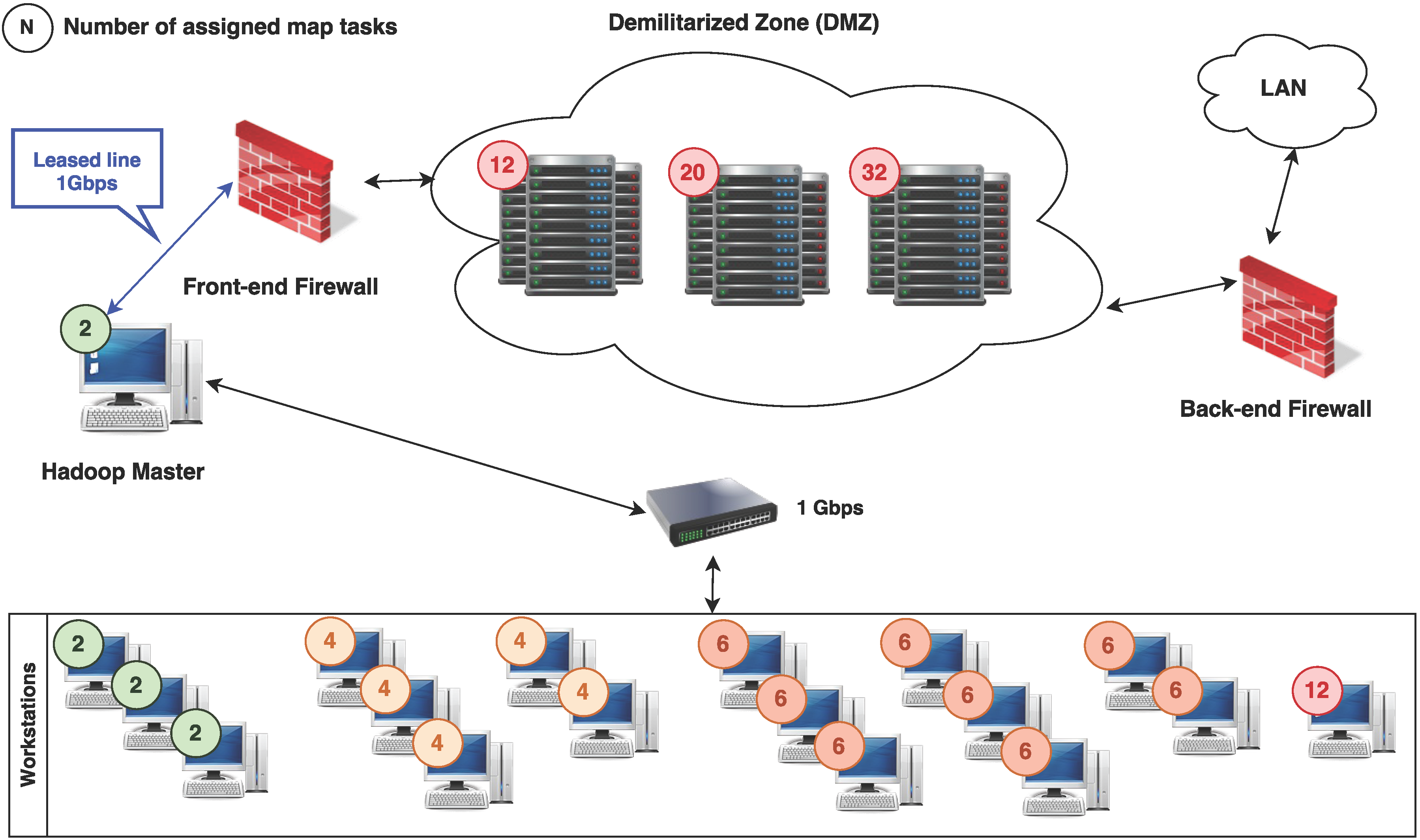
In this article, we describe a very practical approach in detail, based on the Hadoop framework that is easy to set up and manage in a small computing environment, but also easily scalable for larger experiments and supported by many cloud infrastructure providers if the locally available resources become insufficient.

3. Material and Methods

This section describes the datasets, tools and experimental setup used for developing and testing the parallel parameter search framework. It also details the testing use-cases used to evaluate the framework and the adaptive criteria for canceling tasks corresponding to parameter combinations leading to suboptimal classification performance.

3.1. Datasets

The medical image classification task used for this article consists of the identification of five lung texture patterns associated with interstitial lung diseases in high-resolution CT images [16]. The image instances consist of 2D 32 × 32 blocks represented in terms of the energies of sixth-order aligned Riesz wavelet coefficients [17,18], yielding a feature space with 59 dimensions when concatenated with 23 intensity-based features. The distribution and visual aspect of the lung tissue types (including the number of hand-drawn Regions of Interest (ROIs), blocks and patients) are detailed in

Table 1. Visual aspect and distribution of the $32\times 32$ blocks per class of lung tissue pattern. A patient may have several types of lung disorders.

Visual Aspect
tissue type	healthy	emphysema	ground glass	fibrosis	micronodules
hand-drawn
Regions of Interest (ROIs)	150	101	427	473	297
$32\times 32$ blocks	5167	1127	2313	3113	6133
patients	7	6	32	37	16

. Going towards full 3D data analysis also increases runtime for this use case even more, but the current data with larger inter-slice distance does not allow for this.

3.2. Existing Tools

The developed framework relied on Apache Hadoop (http://hadoop.apache.org/, as of 24 February 2016) and can be used with any kind of parameter search problem. Hadoop is a distributed storage and computation tool that supports the MapReduce programming model made popular by Google [19] (among others, such as Apache Spark or Apache Storm). Use of Hadoop is frequent in medium-sized research groups in data science, as it is quick and easy to set up and use, also on heterogeneous infrastructures.

The MapReduce model is used in the context of our experiments, as it is simple and fits our needs well. It separates large tasks into 2 phases, called “Map” and “Reduce”. In a typical setting, the “Map” phase splits a set of input data into multiple parts, which are further processed in parallel and produce intermediate outputs. The “Reduce” phase aggregates the intermediate outputs to produce the final job result. In the context of this article, we only implemented the “Map” phase, as no aggregation was required on the output of this first phase.

Hadoop consists of two main components. The first is a distributed data storage system called Hadoop Distributed File System (HDFS) that manages the storage of extremely large files in a distributed, reliable and fault-tolerant manner. It was used for data input and output when running computations. A detailed description of HDFS can be found in [20]. The second component is the distributed data processing system that was called Hadoop MapReduce in early versions of the software and Yet Another Resource Negotiator (YARN) since Version 2.0 of Hadoop. The reason behind the name change is that the programming algorithm was decoupled from the execution framework in the second generation of Hadoop, allowing for more flexible use of different distributed programming paradigms, i.e., it is not restricted to the batch-oriented MapReduce framework [21] anymore. This can also provide opportunities for making the developed framework evolve towards new paradigms and use-cases.

The synchronization of distributed parallel tasks was performed with Apache ZooKeeper (http://zookeeper.apache.org/, as of 24 February 2016). The focus of this tool is to provide highly reliable distributed coordination [22]. The architecture of ZooKeeper supports redundancy and can therefore provide high availability. The data are stored in the computation nodes and are saved under hierarchical name spaces, similar to a file system or other tree structures.

The simulation tool used for estimating the runtime of a Hadoop job under given conditions (as well as tweaking the parameters of the experiments) was programmed in Java and is detailed in Section 4.2. It uses the output of one full Hadoop job as a baseline for running simulations. The WEKA Data Mining Software [23] was used for the implementation of the SVM and RF classifiers.

3.3. Hardware and Hadoop Cluster

The in-house Hadoop cluster consisted of:

• 21 nodes including a majority of 8-core CPU desktop stations with 16 Gigabytes (GBs) of Random–Access Memory (RAM), as well as 4 more powerful machines (24 cores and 64GB of RAM, 24 cores and 96GB of RAM, 40 cores and 128GB of RAM, 64 cores and 128GB of RAM).
• Gigabit Ethernet network connections between all nodes.
• a total of 152 simultaneous Map tasks (number of cores attributed to Hadoop in the cluster) and 26 simultaneous Reduce tasks. The total is given by the number of tasks that were assigned to the Hadoop cluster on each node, both for the Map and Reduce phases.

Figure 1 shows a schema of the cluster of machines, listing all of the nodes and the network configuration, as well as the number of Map tasks assigned to each computer, as nodes are configured according to their computing power. All desktop machines are commonly used by researchers during the day; therefore, only a subset (usually about 50%) of CPU cores and main memory are attributed to the Hadoop cluster. Previous research showed that the daily normal usage of machines has little impact on the duration of Hadoop jobs in our environment [3].

3.4. Classification Algorithms

Two classification algorithms were used and optimized for the categorization of the lung tissue types: SVMs and RFs. An extension to other tasks is easily possible, but these two are characteristic for many other techniques, and both are frequently used in machine learning and medical imaging.

SVMs has been shown to be effective to categorize texture in wavelet feature spaces [24] and in particular for lung tissue [25]. Kernel SVMs implicitly maps feature vectors $v_i$ to a higher-dimensional space by using a kernel function $K(v_i,v_j)$. We used the RBF kernel given by the multidimensional Gaussian function:

$$K(v_i,v_j)=e^{\frac{-\left|\right|v_i-v_j{\left|\right|}^2}{2\gamma }}$$

(1)

SVMs builds separating hyperplanes in the higher-dimensional space considering a two-class problem. Two parallel hyperplanes are constructed symmetrically on each side of the hyperplane that separates the two classes. The goal of SVMs is to maximize the distance between the two external hyperplanes, called the margin [26]. This yields the decision function $f\left(v_i\right)$, which minimizes the functional:

$${\left|\right|f\left|\right|}_K+C\sum _{i=1}^{N}max{(0,1-y_{i}f\left(v_i\right))}^2$$

(2)

with ${\left|\right|f\left|\right|}_K$ the norm of the reproducing kernel Hilbert space defined by the kernel function K, N the total number of feature vectors and $y_i$ the class labels (i.e., $y_i\in \{-1,1\}$). The parameter C determines the cost attributed to errors and requires optimization to tune the bias-variance trade-off. For multiclass classification, several one-versus-all classifiers are built, and the model with the highest decision function determines the predicted class. Two parameters are being optimized for SVMs: the cost C and the parameter of the Gaussian kernel γ.

RFs consists of building ensembles of Decision Trees (DTs) [27]. Each DT is built on a subset of features and a subset of training vectors (i.e., bagging). The DTs divides the feature space successively by choosing primarily features with the highest information gain [28]. The final class prediction of RFs is obtained as the mean prediction of all individual trees. Three parameters are being optimized for RFs, the number of generated random trees T, and for each DT, the number of randomly-selected features F and the maximum tree depth D.

3.5. Task Cancellation Criteria

The following is a description of the method used for deciding which hyperparameter combinations to keep during the execution of the experiments on the Hadoop cluster. The classification accuracy $ac{c}_k$ associated with one set of hyperparameters is monitored throughout the execution of the k folds of the CV. In order to determine if a hyperparameter combination is performing well, the first considered criterion is whether the value of $acc$ appears to be stable for the given combination over the k folds of the CV. The mean accuracy ${\mu }_{acc}$ is updated each time a new value for this hyperparameter combination is available (i.e., each time that a new fold of the CV has completed) and added to a list of values. At the same time, the variance ${\sigma }_{acc}$ is calculated for the set of recorded mean accuracies over a “sliding window” of size $W_k$. Finally, the gradient of the variance is determined over these $W_k$ values as $\frac{\partial {\sigma }_{acc}}{\partial k}$, $k\in [1,\cdots ,W_k]$. $\frac{\partial {\sigma }_{acc}}{\partial k}$ was computed using least squares regression. If the gradient is $\frac{\partial {\sigma }_{acc}}{\partial k}<=0$, the estimated classification accuracy was considered to be stable; otherwise, the evolution of the mean accuracy is deemed to be unstable, and no decision is made yet about the cancellation of this combination. When the accuracy is found to be stable, the second step consists of comparing one or more criteria of the current combination of parameters against the global evolution of the classification accuracy given by all other parameter combinations. Two criteria are considered:

• Is the current mean accuracy of the combination ${\mu }_{acc}$ lower than the global mean accuracy (minus a margin of ${\mathsf{\Delta }}_{acc}$)?
• Is the current mean runtime of 1 task for the combination longer than the global mean runtime for 1 task (multiplied by a factor of ${\mathsf{\Delta }}_t$)?

The first criterion is monitoring the accuracy of the current hyperparameter combination. Given that ${\sigma }_{acc}$ is considered to be stable, the chance that the accuracy associated with this combination of parameters improves significantly later is relatively small. Therefore, the combination is canceled if its current accuracy is lower than the current global accuracy. The second criterion works in a similar fashion, but is based on the runtime of the tasks. Indeed, for certain classifiers, such as SVMs, the longer the time to achieve convergence, the higher the likelihood of a bad performance [3]. For this reason, abnormally time-consuming parameter combinations are also canceled, because they generally yield suboptimal results and more importantly have a significant impact (as much as one order of magnitude higher than average runtimes) on the overall runtime of the experiment when not canceled. ${\mathsf{\Delta }}_{acc}$ and ${\mathsf{\Delta }}_t$ can be tuned to balance between overall computational time and classification performance. Additionally, each criterion can be individually enabled or disabled, as not all classifiers follow the same behavior. Algorithm 1 outlines the process described above, with current mean values for the accuracy and runtime being obtained first (both global and for the given parameter combination $pComb$), followed by the set of variances of size $W_k$. Subsequently, the stability test described in this section is performed, as well as the performance checks (accuracy and runtime) in case of a stable evolution. If the combination is performing poorly, its status is set to ‘canceled’. Figure 2 shows an illustration of how the cancellation process works with 3 parameter combinations: a well-performing combination, a combination with suboptimal accuracy and a combination with above-average runtime.

Algorithm 1 Parameter combination cancellation.

1: function cancelParameter($pComb$) 2:     ${\mu }_{\mathit{accGlobal}}\leftarrow$ currGlobalMeanAcc() 3:     ${\mu }_{\mathit{acc}}\leftarrow$ currMeanAcc($\mathit{pComb}$) 4:     ${\mu }_{\mathit{timeGlobal}}\leftarrow$ currGlobalMeanRuntime() 5:     ${\mu }_{\mathit{time}}\leftarrow$ currMeanRuntime($\mathit{pComb}$) 6:     $\mathit{setOf}{\sigma }_{\mathit{acc}}\leftarrow$ currVarsOfMeanAccs($\mathit{pComb}$) 7:     if varIsStable($\mathit{setOf}{\sigma }_{\mathit{acc}}$) then 8:         if ${\mu }_{acc}<{\mu }_{accGlobal}-{\mathsf{\Delta }}_{acc}$ or ${\mu }_{\mathit{time}}>{\mu }_{\mathit{timeGlobal}}-{\mathsf{\Delta }}_t$ then 9:            $pComb.status{\leftarrow }^{\prime }{\mathtt{canceled}}^{\prime }$ 10:         end if 11:     end if 12: end function

4. Results

This section describes the implementation of the framework and the experimental results obtained.

4.1. Implementation of the Hadoop-Based Execution Framework

4.1.1. Standard Run

The following list outlines all of the chronological steps for running a distributed parameter search using the framework, but without optimization (i.e., no task cancellation). This is referred to as the standard run.

• An input file containing a hash table with all of the possible combinations of parameter values and patient identifiers (the latter was used for performing a Leave–One–Patient–Out (LOPO) CV) is created (one combination per line). This hash table was based on parameter ranges specified by the user. In the case of a random search, the user simply specifies the lower and upper bounds of each parameter, the values are then generated randomly within this space. The order of the lines was randomized in order to avoid executing a large number of similarly complex tasks at the same time. The file is then uploaded to the HDFS, where it serves as the input file of the Hadoop job.
• The Hadoop job starts, splitting the workload into $N/M$ Map tasks, where N is the total number of lines in the file and M is a variable defining how many lines a single task should process. M can be tweaked in order to avoid having Map tasks that are extremely short (less than 10 seconds). Map tasks that are too short can impact the runtime of a Hadoop job in a non-negligible fashion due to overhead caused by starting and managing Hadoop tasks.
• Each task executes a setup function (only once per Map task) that contains the following steps:

  (a)

  Load the dataset and prepare it for use (in this case, set the instance class attribute).

  (b)

  Normalize the dataset: the feature values were scaled to $[0,1]$.

• Each task executes the Map function (M times per task) that consists of one fold of the LOPO CV:

  (a)

  Split the data into a training set containing all of the instances of the dataset except for those of the current patient and a testing set containing all of the instances of the current patient.

  (b)

  Build the classifier using the current combination of parameters (for example, C and γ in the SVM use-case) and the training set.

  (c)

  Classify each instance of the test set using the previously-built classifier model.

  (d)

  Get the number of total and correctly-classified instances and write them as the output of the function.

The above process is shown in Algorithm 2.

Algorithm 2 Execution framework: standard run.

1: generateInput() 2: startJob() 3: for all $\mathit{task}\in N/M_{\mathit{tasks}}$ do 4:     loadDataset()         → Setup ($1\times$ per task) 5:     prepareDataset() 6:     normalizeDataset() 7:     for all $\mathit{pComb}\in M_{\mathit{pCombinations}}$ do         → Map ($M\times$ per task) 8:         $\mathit{tStart}\leftarrow \mathbf{NOW}$ 9:         $\mathit{classifierArgs}\leftarrow \mathit{pComb}.\mathit{classifierArgs}$ 10:         $\mathit{patientID}\leftarrow \mathit{pComb}.\mathit{patientID}$ 11:         configureClassifier($\mathit{classifierArgs}$) 12:         splitDataSet($\mathit{patientID}$)         → LOPO 13:         trainClassifier($\mathit{trainingSet}$) 14:         $\mathit{result}\leftarrow$classifyTestSet($\mathit{testSet}$) 15:         $\mathit{tEnd}\leftarrow \mathbf{NOW}$ 16:         $\mathit{acc}\leftarrow \mathit{result}.\mathit{correct}/\mathit{result}.\mathit{total}$ 17:         $\mathit{runtime}\leftarrow \mathit{tEnd}-\mathit{tStart}$ 18:         writeOutput($\mathit{acc},\mathit{result}.\mathit{correct},\mathit{result}.\mathit{total},\mathit{patientID},\mathit{runtime}$) 19:     end for 20: end for

4.1.2. Optimized Run

When activating the mode that cancels suboptimal tasks (referred to as optimized run, see Section 3.5), the process was slightly modified:

• Before the job starts, various “znodes” (i.e., znodes are files persisting in memory on the ZooKeeper server) are initialized for storing parameter combination accuracy values, a list of canceled parameter combinations, etc.
• During the setup (Point 3 of the previous list), a connection to the ZooKeeper object is established, and the variables for canceling tasks are attributed.
• At the start of the Map function (Point 4 of the previous list), a check is performed to identify if the parameter combination was already canceled. If this is the case, the function returns immediately; otherwise, the classification is performed as usual.
• Once the classification is finished, several values in the ZooKeeper server are updated:

  (a)

  The number of total and correctly-classified instances, as well as the runtime of the tasks for the given parameter combination are incremented.

  (b)

  The current accuracy of the given parameter combination was added to the DescriptiveStatistics object (part of the Apache Commons Math library (http://commons.apache.org/proper/commons-math/, as of 24 February 2016)), which allows easy calculations of statistical values (e.g., ${\mu }_{acc}$, ${\sigma }_{acc}$) on an evolving set of data.

  (c)

  The current variance ${\sigma }_{acc}$ (computed from all existing accuracies for the given parameter combination) is added to a circular buffer of size $W_k$. This buffer is further used to calculate the gradient of the variance evolution over the last $W_k$ values.

  (d)

  The number of total and correctly classified instances, as well as the runtime of the tasks for the global job are incremented.

• At the end of the Map function, a check is performed whether the current parameter combination needs to be canceled or not. This check takes into account the following variables:

  (a)

  Variance over the last $W_k$ values is stable, i.e., $\frac{\partial {\sigma }_{acc}}{\partial k}<=0$. If the gradient is positive, it is assumed that the values are still changing significantly and the parameter combination is not canceled.

  (b)

  Mean accuracy of the given parameter combination. If ${\mu }_{acc}$ is smaller than the mean global accuracy of all parameter combinations minus a ${\mathsf{\Delta }}_{acc}$ (set to $0.05$ in our experiments), the parameter combination is canceled (or blacklisted), i.e., the classification step in all subsequent Map tasks of the corresponding parameter combination will not be executed.

  (c)

  Mean runtime of the given parameter combination. If the latter is longer than the mean global runtime of all parameter combinations multiplied by a ${\mathsf{\Delta }}_t$ (set to $2.0$ in our experiments), the parameter combination is canceled, i.e., the classification step in subsequent Map tasks of the corresponding parameter combination is not executed.

The above process is shown in Algorithm 3, where differences with the standard run (Algorithm 2) are highlighted.

Algorithm 3 Execution framework: optimized run (differences with Algorithm 2 are highlighted).

1: generateInput() $2:$ $\mathrm{initSyncFields}\left(\right)$ 3: startJob() 4: for all $\mathit{task}\in N/M_{\mathit{tasks}}$ do 5:     loadDataset()         → Setup ($1\times$ per task) 6:     prepareDataset() 7:     normalizeDataset() $8:$     $\mathrm{initStatsObjects}\left(\right)$ 9:     for all $\mathit{pComb}\in M_{\mathit{pCombinations}}$ do         → Map ($M\times$ per task) $10:$          $\mathbf{if}\mathit{pComb}.\mathit{status}{=}^{\prime }{\mathtt{canceled}}^{\prime })\mathbf{then}$ $11:$            $\mathbf{continue}$          $\to \mathrm{Skip canceled iterations}$ $12:$         $\mathbf{end}\mathbf{if}$ 13:         $\mathit{tStart}\leftarrow \mathbf{NOW}$ 14:         $\mathit{classifierArgs}\leftarrow \mathit{pComb}.\mathit{classifierArgs}$ 15:         $\mathit{patientID}\leftarrow \mathit{pComb}.\mathit{patientID}$ 16:         configureClassifier($\mathit{classifierArgs}$) 17:         splitDataSet($\mathit{patientID}$)         → LOPO 18:         trainClassifier($\mathit{trainingSet}$) 19:         $\mathit{result}\leftarrow$classifyTestSet($\mathit{testSet}$) 20:         $\mathit{tEnd}\leftarrow \mathbf{NOW}$ 21:         $\mathit{acc}\leftarrow \mathit{result}.\mathit{correct}/\mathit{result}.\mathit{total}$ 22:         $\mathit{runtime}\leftarrow \mathit{tEnd}-\mathit{tStart}$ 23:         writeOutput($\mathit{acc},\mathit{result}.\mathit{correct},\mathit{result}.\mathit{total},\mathit{patientID},\mathit{runtime}$) $24:$         $\mathrm{updateSyncFields}(\mathit{pComb},\mathit{result}.\mathit{correct},\mathit{result}.\mathit{total},\mathit{runtime})$ $25:$         $\mathrm{cancelParameter}\left(\mathit{pComb}\right)$ 26:     end for 27: end for

4.2. Implementation of the Simulation Tool

Time is often a limiting factor when running experiments, and it can have a strong influence on the achieved results. Having a tool that can run simulated grid search experiments (modeled after the real-world Hadoop-based framework) in a single machine in order to approximate runtime and give indications about the expected performance can help in designing experiments, choosing sensible margins for parameter cancellation (see Section 3.5), estimating the required scale of a computation cluster, as well as calculating the cost of running the experiment in a cloud-based “pay-as-you-go” platform. This section details the implementation of this tool: the behavior of the real-world Hadoop implementation was closely reproduced, with the following characteristics and differences:

• The results of a Hadoop experiment (containing the runtime of each task) are loaded into the simulator Java class: they will serve as a baseline for simulating Hadoop jobs with different amounts of available computation tasks and different values for the termination criteria margins, for example.
• A “time step” counter is initialized and incremented in milliseconds, simulating the passage of time.
• A queue of running tasks (of size T, representing the number of Map tasks in the simulated cluster) is populated.
• After each millisecond, the starting/ending tasks are managed and the cancellation checks are performed like on the Hadoop cluster. The major difference is that instead of using the ZooKeeper distributed synchronization system, simple Java data structures are used (hash maps, lists, etc.) for monitoring the evolution of parameter combination performance.
• Each time a task completes, another pending task is added to the queue of running tasks. This behavior is the same as in Hadoop.
• At the end of the simulated Hadoop job (all tasks are processed), statistics about the simulated job are given as an output: total duration of the job (if executed in a real cluster of a given size), number of canceled parameters, maximum achieved accuracy, etc.

The goal is to have a tool that can provide an approximation of the average runtime of a task for a given machine learning scenario, including the variance in processing time for different parameter values. A real small-scale experiment with a coarse grid can be run to get a clear idea of these values, that can then serve as a base for a simulated experiment at a much larger scale. If running a real experiment before simulation is not desired or feasible, the tool can also easily use an average runtime per task (with margins to represent shorter and longer tasks) directly input by the user after performing some local empirical tests.

4.3. Experimental Results

Several experiments were performed:

• Determining the speedups that can be obtained (with and without task cancellation) compared to a serial execution on a single computer.
• Verifying whether the best parameter combination is kept when canceling tasks.
• Comparing the runtime and performance between grid and random search.
• Investigating if the developed simulation tool can provide a realistic approximation of the runtime of an experiment under varying conditions.

4.3.1. Grid Search

The first experiments were conducted with the classical grid parameter search strategy. All of the experiments were run using the Hadoop cluster configuration described in Section 3.3. When the objective function (e.g., classification accuracy) is expected to be smooth through consecutive parameters, the grid search is expected to lead to reproducibly good results with a trade-off between grid size and the probability to find the maximum performance (or be at least very close to it).

For both use-cases (RF and SVM), the Hadoop job was run twice: once based on the standard run mode, where no tasks were canceled during the execution of the job, and once based on the optimized run mode, where tasks corresponding to suboptimal parameter combinations were canceled. The results are presented in

Table 2. Experimental results showing the comparison between an estimation of running the grid parameter search on a single computer and running it on the in-house Hadoop cluster in the standard run and optimized run configurations, for both use-cases (RF and SVM). The indication in brackets [ ... ] for the “best accuracy” value in the optimized run column shows whether the best or second best achieved accuracy of the standard run was kept running.

Random Forest (RF) Optimization
	Single Computer	Hadoop Cluster	Hadoop Cluster
	(Estimation)	(Standard Run)	(Optimized Run)
Job execution time	302 d 00 h 15 m 24 s	51 h 27 m 03 s	19 h 52 m 05 s
Total combinations	651,460	651,460	651,460
Lines per task	N/A	20	20
Total Map tasks	N/A	32,573	32,573
Number of canceled parameter combinations	N/A	0	5052/7500
Best accuracy	0.73762	0.73762	0.73756 (2nd best)
Speedup	1×	~141×	~364×
Support Vector Machine (SVM) Optimization
	Single Computer	Hadoop Cluster	Hadoop Cluster
	(Estimation)	(Standard Run)	(Optimized Run)
Job execution time	52 d 17 h 27 m 10 s	8 h 49 m 51 s	4 h 40 m 57 s
Total combinations	38,786	38,786	38,786
Lines per task	N/A	2	2
Total Map tasks	N/A	19,393	19,393
Number of canceled parameter combinations	N/A	0	236/451
Best accuracy	0.77999	0.77999	0.77999 (best)
Speedup	1×	~143×	~270×

. An estimation of the time required to run the computation serially on a single computer is provided in the first column. The estimation is based on the runtime recorded for each Map task, purely for the classification part, therefore excluding the overhead produced by Hadoop for starting and managing tasks.

The grid parameter search domain is defined as follows:

• For the SVM use-case, two parameters are being optimized.

  • The cost C, varying from zero to 100 in increments of 10 (and $C=0$ is replaced with $C=1$).
  • The kernel parameter G, varying from $-2.0$ to $2.0$ in increments of $0.1$ (actual kernel value is computed by $\gamma ={10}^G$).
• For the RF use-case, three parameters are being optimized.

  • The number of trees in the random forest T, varying from zero to 1000 in increments of 10 (and $T=0$ is replaced with $T=10$).
  • The maximum tree depth D, varying from zero to four in increments of one (where $D=0$ signifies that the depth is not restricted).
  • The number of randomly-selected features F for testing at each node, varying from one to $2*\sqrt{N}$ in increments of one (where N is the total number of features, in this case 58).

4.3.2. Random Search

Two more experiments were run using the random search strategy for the SVM use-case in order to demonstrate the flexibility of the developed framework and to investigate the possible improvements in terms of runtime and maximum achieved classification accuracy. Very good and efficient results were reported for random search in the past despite the fact that the results are not necessarily reproducible, and thus, non-optimal results are a risk, albeit with low probability [2]. In order to allow fair comparisons with grid search, the same number of points used was generated randomly in the search space based on a uniform distribution, using the same upper and lower bounds. The comparison of the results is shown in

Table 3. Comparison between running a grid parameter search and a random search (with the same number of combinations), with and without task cancellation, for optimizing the hyper-parameters of the SVM experiment.

Grid search and random search comparison: Support Vector Machine (SVM) experiment
	Grid search (standard run)	Random search (standard run)	Grid search (optimized run)	Random search (optimized run)
Job Execution time	8 h 49 m 51 s	8 h 14 m 32 s	4 h 40 m 57 s	4 h 08 m 44 s
Number of canceled parameter combinations	0	0	236 / 451	254/451
Best accuracy	0.77999	0.78033	0.77999	0.78045

. The runtimes and results are in this case very close to the ones obtained with the grid search.

A series of random search experiments using a varying number of randomly-sampled points were also conducted, in order to analyze the evolution of both the runtime of the Hadoop job, as well as the maximum achieved accuracy. The results are shown in Figure 3.

Finally, multiple iterations (20 in total) of the same random search experiment (using 25% of the original number of points, i.e., 112 combinations) were run in order to determine the Relative Standard Deviation (RSD) of the maximum accuracy obtained, as well as the job runtime. The results are shown in Figure 4.

4.4. Simulation Results and Validation

Once the output of a standard run was available, it was fed into the simulation tool to estimate the runtime of the same job under different conditions. For instance, the number of simultaneous Map tasks can be increased to approximate the runtime on a larger Hadoop cluster. Similarly, the ${\mathsf{\Delta }}_{acc}$ and ${\mathsf{\Delta }}_t$ task cancellation margins can be adjusted to evaluate the time-performance trade-off (i.e., smaller margins will lead to faster runtimes, but increase the risk of canceling optimal parameter combinations).

To validate whether the simulation tool can produce realistic results, the SVM grid search use-case was executed four times in the Hadoop cluster:

• standard run and optimized run with 152 Map tasks, ${\mathsf{\Delta }}_{acc}=0.05$ and ${\mathsf{\Delta }}_t=2.0$.
• standard run and optimized run with 64 Map tasks, ${\mathsf{\Delta }}_{acc}=0.05$ and ${\mathsf{\Delta }}_t=2.0$.

The results of the first two executions with 152 tasks are used as the input for running four simulations with the same number of Map tasks as the runs listed above. The results are shown in

Table 4. Validation of the simulation tool.

Support Vector Machine (SVM): standard run
	Experimental result	Simulation result	Relative difference
152 Map tasks (baseline)	9 h 26 m 04 s	9 h 17 m 56 s	$-1.43\%$
64 Map tasks	19 h 42 m 31 s	21 h 39 m 57 s	$+9.93\%$
SVM - optimized run
	Experimental result	Simulation result	Relative difference
152 Map tasks (baseline)	4 h 40 m 57 s	5 h 16 m 19 s	$+12.58\%$
64 Map tasks	9 h 24 m 54 s	12 h 17 m 49 s	$+30.61\%$

. A fixed three-second overhead (determined by empirical tests) was added to the runtime of each task in order to simulate the impact of Hadoop task setup. Moreover, an interesting opportunity provided by the simulation tool is to evaluate the effect of the cancellation margins ${\mathsf{\Delta }}_{acc}$ and ${\mathsf{\Delta }}_t$ on the maximum accuracy achieved. By gradually changing these values for the results of the SVM grid search experiment, Figure 5 and Figure 6 are created. Results with cancellation are less precise in the simulations compared to results without task cancellations.

5. Discussion

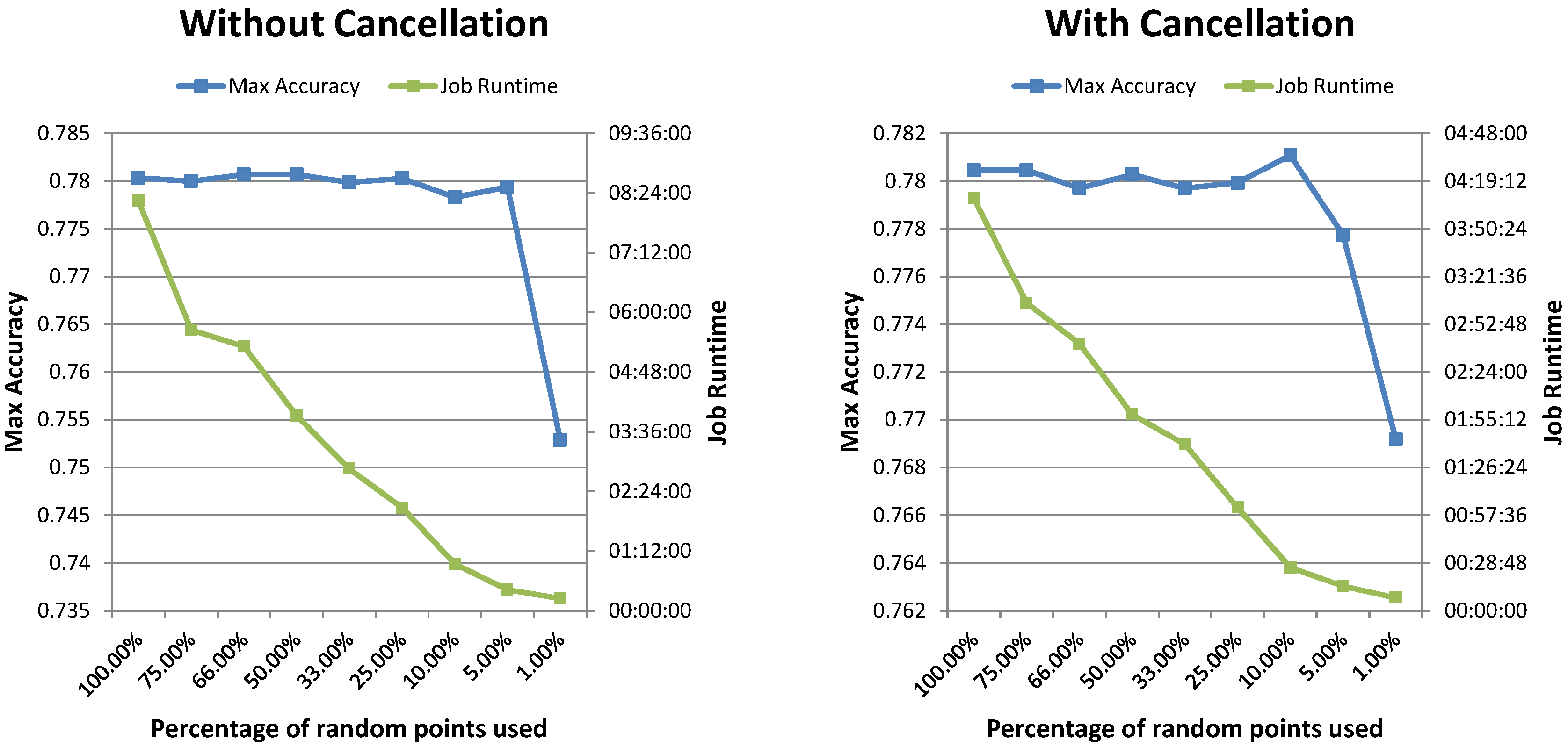
Three major observations can be deduced from the experimental results: first of all, the speedup achieved by simply distributing a grid parameter search is very substantial, with the total runtime for the search accelerated by a factor of 141× (RF) and 143× (SVM), when compared to an estimation of a serial execution on a single computer (see Table 2). It also shows that the total runtime decreases almost linearly as the number of nodes (and therefore, available Map tasks) in the Hadoop cluster increases. Second, adding the accuracy and runtime check and canceling suboptimal parameter combinations allows decreasing the runtime even further, by a factor close to or greater than 2× in both use-cases without any significant impact on the maximum achieved accuracy. It also shows that the framework performed well for two different types of classifiers and with a different number of hyperparameters. Third, the results show that several parameter search strategies are supported and work well with the developed framework. 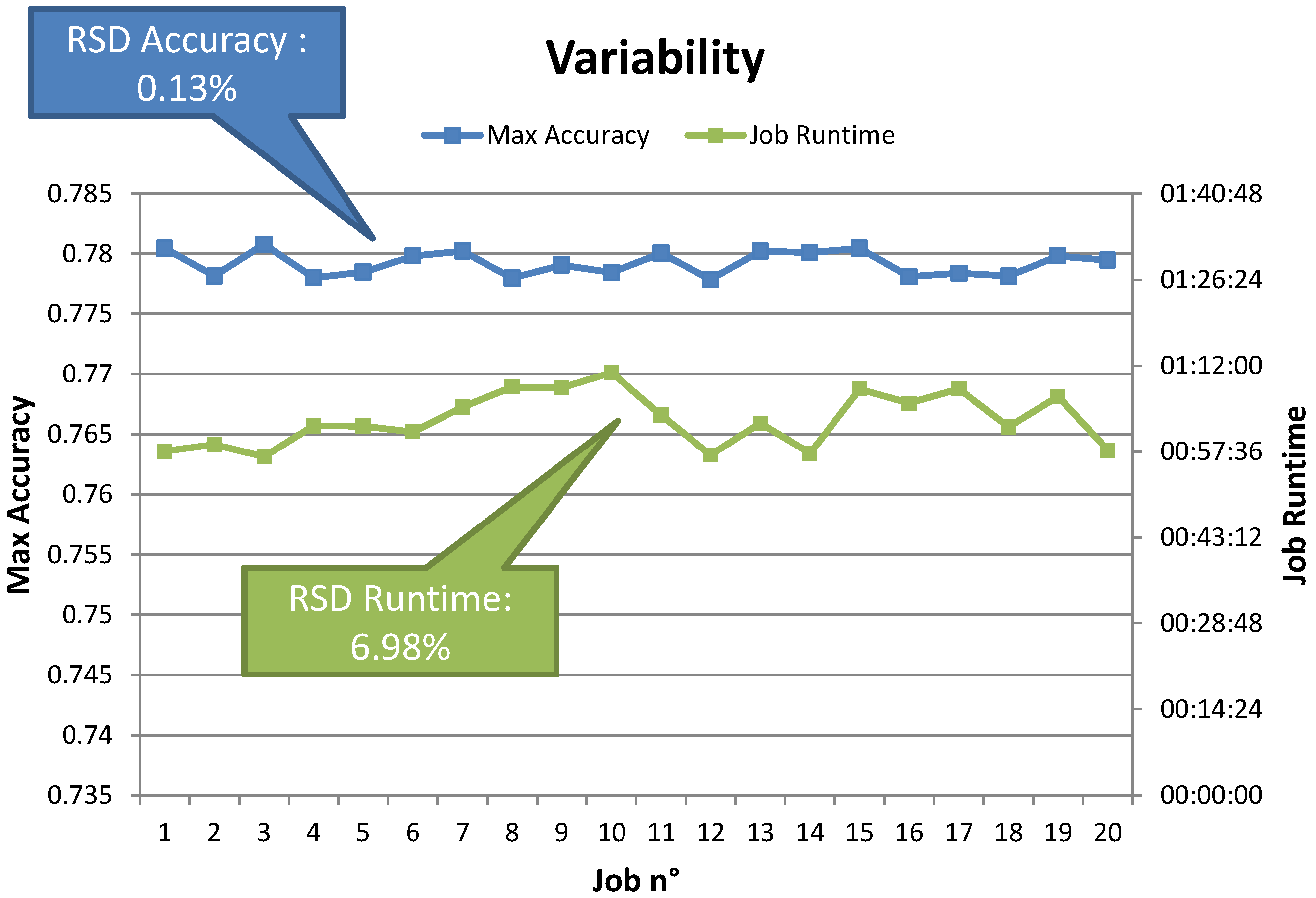The random search experiments ran slightly faster than the grid search using the same number of points and gave equivalent results both with and without task cancellation (see Table 3). Moreover, reducing the number of random points yielded equivalent results in a fraction of the time needed for the grid search experiments. Repeated experiments also showed that the variability in terms of runtime and achieved performance is minimal. Random search thus provides an interesting option, also in the simulation tool.

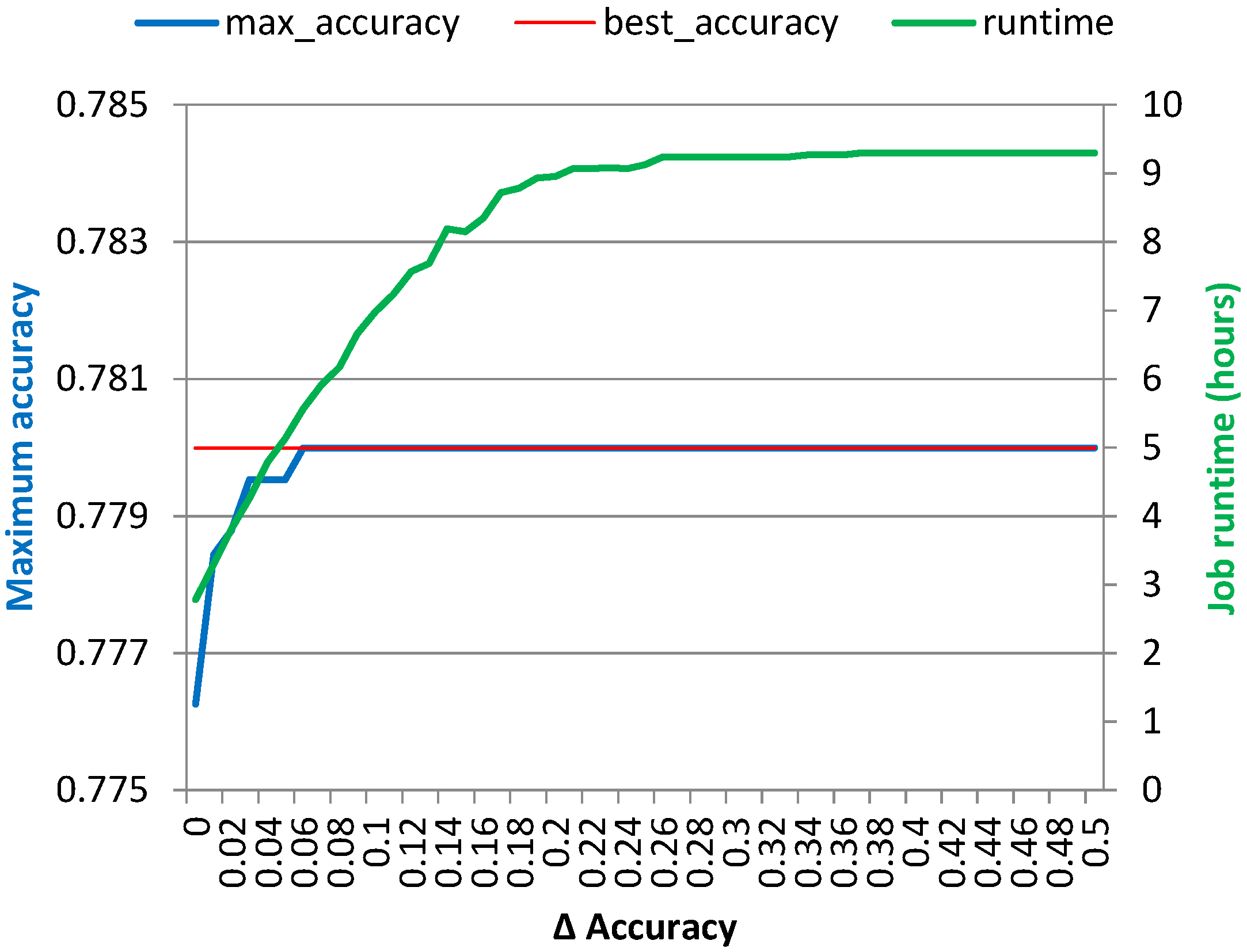
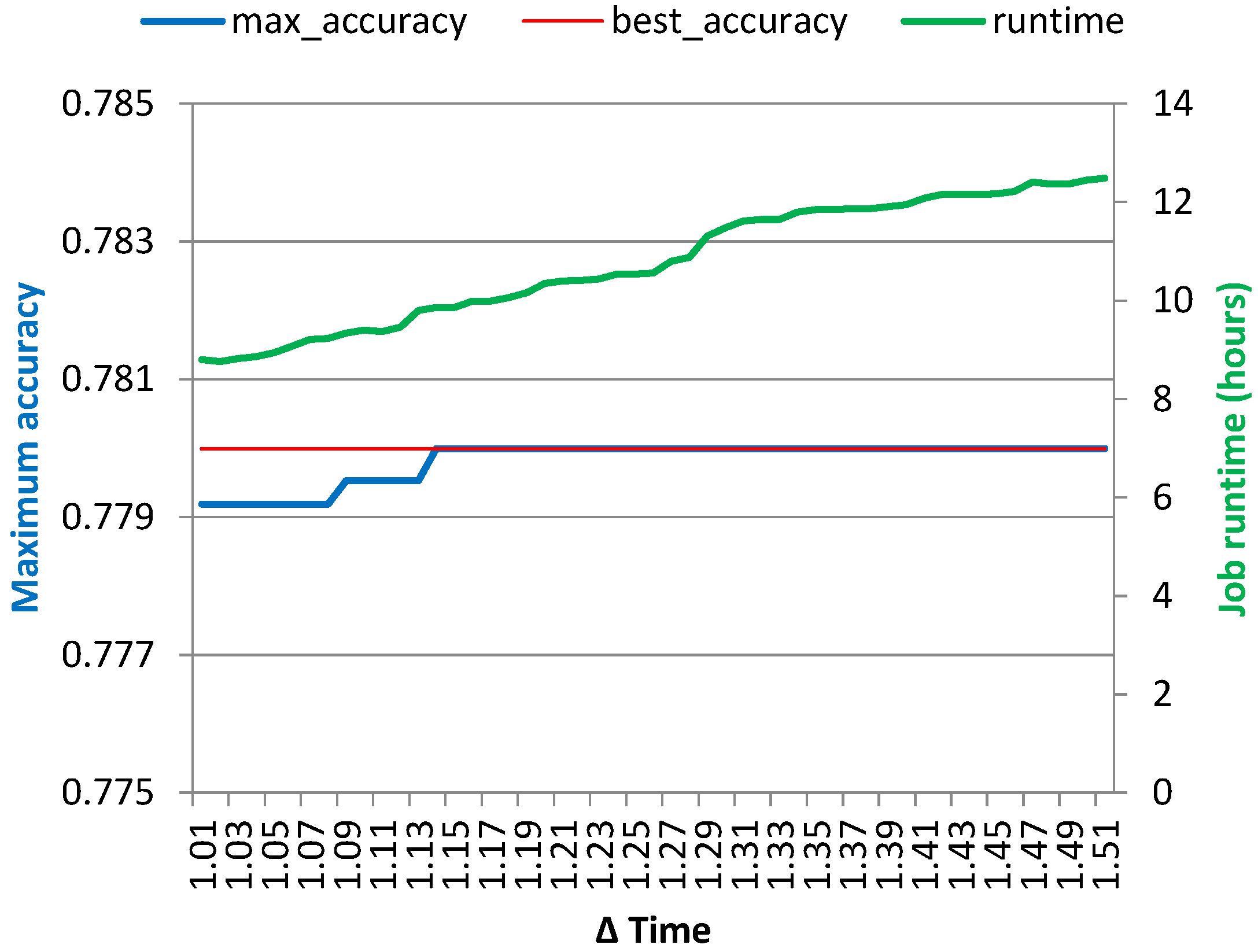
The proposed simulation tool was successfully used to estimate job runtimes using a varying number of tasks, with a relative difference of ~10% between the real-world experiment and the simulation for the standard run using a smaller number of simultaneous tasks (64; see Table 4). For the optimized run, the errors were larger, about ~12.5% when simulating with the original amount of Map tasks and ~30.6% when using the smaller number of tasks. Moreover, the simulation provided insights into the effect of varying the cancellation conditions on the maximum achieved classification accuracy and overall job runtime without requiring running a battery of lengthy Hadoop jobs. The latter can be used to reduce costs when using “pay-as-you-go” computing resources in the cloud, which might in the future become the main computation source for many research departments in any case.

Some limitations of this work include the LOPO CV, which could benefit from an added inner Cross–Validation (CV) performed on the training set, in order to reduce the risk of overfitting. Fortunately, this is entirely possible with our framework and is well-suited for parallelizing the task even further. Another limitation concerns the simulation tool, which currently works based only on the results of a real-world experiment. Although it is still interesting to use it on a small-scale experiment and then to extrapolate the data to a more exhaustive experiment, the tool could benefit from a completely simulated mode, where tasks are generated dynamically using an average runtime of tasks input by the user (and adapted with various factors to better represent the variability in runtime of a given experiment and the execution on a distributed framework).

6. Conclusions

The developed framework allows speeding up hyperparameter optimization for medical image classification significantly and easily (both for grid search and random sampling). The distributed nature of the execution environment is leveraged for reducing the search space and gaining further wall time. The simulation tool allows estimating the runtime and results of medical texture analysis experiments under various conditions, as well as extracting information such as a measure of the time-performance trade-off of varying the cancellation margins. These tools can be used in a large variety of tasks that include both image analysis and machine learning aspects. The system using Hadoop is relatively easy to set up, and we expect that many groups can make such optimizations in a much faster way using the results of this article. Indeed, the dramatic reduction in runtime using only a local computing infrastructure can enable the execution of experiments at a scale that may have been dismissed previously, ensuring one to get the best-possible results in the optimization of classification or similar tasks in a very reasonable amount of time. The simulation environment can also help analyze performance and cost trade-offs when optimizing parameters and potentially using cloud environments, allowing one to give cost estimates.

The framework was evaluated with machine learning algorithms with a small number of hyperparameters (i.e., two for SVMs and three for RFs).

In future work, the framework is planned to be tested with other datasets and more classifiers in order to validate its flexibility, potentially also with approaches, such as deep learning, that can use several million hyperparameters and usually rely on GPU computing [29], often supported by cloud providers, as well. It is also planned to run comparative and larger-scale experiments on a cloud-computing platform instead of using the local Hadoop infrastructure to compare the influence of a mixed environment on runtime, as this can depend much more on the available bandwidth. More advanced task cancellation criteria could also be implemented (e.g., bandit-based method) to allow for more fine-grained control over the tasks to keep. Moreover, adding more sophisticated parameter search strategies to the framework, such as Bayesian optimization or gradient descent, could help improve the system even further, even though it will increase the complexity.

References

1. Kim, J. Iterated Grid Search Algorithm on Unimodal Criteria. Ph.D. Thesis, Virginia Polytechnic Institute and State University, Blacksburg, VA, USA, 1997. [Google Scholar]
2. Bergstra, J.; Bengio, Y. Random Search for Hyper-parameter Optimization. J. Mach. Learn. Res. 2012, 13, 281–305. [Google Scholar]
3. Markonis, D.; Schaer, R.; Eggel, I.; Müller, H.; Depeursinge, A. Using MapReduce for Large–scale Medical Image Analysis. 2015. Available online: http://xxx.lanl.gov/abs/arXiv:1510.06937 (accessed on 31 May 2016). [Google Scholar]
4. Owen, S.; Anil, R.; Dunning, T.; Friedman, E. Mahout in Action; Manning Publications Co.: Greenwich, CT, USA, 2011. [Google Scholar]
5. Luo, G. MLBCD: A machine learning tool for big clinical data. Health Inf. Sci. Syst. 2015, 3, 3. [Google Scholar] [CrossRef] [PubMed]
6. Hutter, F.; Hoos, H.H.; Leyton-Brown, K. Sequential Model-based Optimization for General Algorithm Configuration. In Learning and Intelligent Optimization; Springer-Verlag: Berlin/Heidelberg, Germany, 2011; pp. 507–523. [Google Scholar]
7. Friedrichs, F.; Igel, C. Evolutionary tuning of multiple SVM parameters. Neurocomputing 2005, 64, 107–117. [Google Scholar] [CrossRef]
8. Thornton, C.; Hutter, F.; Hoos, H.H.; Leyton-Brown, K. Auto-WEKA: Combined Selection and Hyperparameter Optimization of Classification Algorithms. In Proceedings of the 19th ACM SIGKDD International Conference on Knowledge Discovery and Data Mining; ACM: New York, NY, USA, 2013; pp. 847–855. [Google Scholar]
9. Snoek, J.; Larochelle, H.; Adams, R.P. Practical Bayesian Optimization of Machine Learning Algorithms. In Advances in Neural Information Processing Systems 25; Pereira, F., Burges, C.J.C., Bottou, L., Weinberger, K.Q., Eds.; Curran Associates, Inc.: Red Hook, NY, USA, 2012; pp. 2951–2959. [Google Scholar]
10. Chapelle, O.; Vapnik, V.; Bousquet, O.; Mukherjee, S. Choosing Multiple Parameters for Support Vector Machines. Mach. Learn. 2002, 46, 131–159. [Google Scholar] [CrossRef]
11. Bergstra, J.S.; Bardenet, R.; Bengio, Y.; Kégl, B. Algorithms for Hyper-Parameter Optimization. In Advances in Neural Information Processing Systems 24; Shawe-Taylor, J., Zemel, R.S., Bartlett, P.L., Pereira, F., Weinberger, K.Q., Eds.; Curran Associates, Inc.: Red Hook, NY, USA, 2011; pp. 2546–2554. [Google Scholar]
12. Gorissen, D.; Couckuyt, I.; Demeester, P.; Dhaene, T.; Crombecq, K. A Surrogate Modeling and Adaptive Sampling Toolbox for Computer Based Design. J. Mach. Learn. Res. 2010, 11, 2051–2055. [Google Scholar]
13. Bergstra, J.; Komer, B.; Eliasmith, C.; Yamins, D.; Cox, D.D. Hyperopt: A Python library for model selection and hyperparameter optimization. Comput. Sci. Discov. 2015, 8, 014008. [Google Scholar] [CrossRef]
14. Sparks, E.R.; Talwalkar, A.; Haas, D.; Franklin, M.J.; Jordan, M.I.; Kraska, T. Automating Model Search for Large Scale Machine Learning. In Proceedings of the Sixth ACM Symposium on Cloud Computing, Kohala Coast, HI, USA, 27–29 August 2015; pp. 368–380.
15. Liu, K.; Zhao, Q. Distributed Learning in Multi-Armed Bandit With Multiple Players. IEEE Trans. Signal Process. 2010, 58, 5667–5681. [Google Scholar] [CrossRef]
16. Depeursinge, A.; Vargas, A.; Platon, A.; Geissbuhler, A.; Poletti, P.A.; Müller, H. Building a Reference Multimedia Database for Interstitial Lung Diseases. Comput. Med. Imaging Gr. 2012, 36, 227–238. [Google Scholar] [CrossRef] [PubMed]
17. Depeursinge, A.; Foncubierta-Rodríguez, A.; Van De Ville, D.; Müller, H. Multiscale Lung Texture Signature Learning Using The Riesz Transform. In Medical Image Computing and Computer–Assisted Intervention MICCAI 2012; Springer: Berlin/Heidelberg, Germany, 2012; pp. 517–524. [Google Scholar]
18. Depeursinge, A.; Foncubierta-Rodríguez, A.; Van De Ville, D.; Müller, H. Rotation–covariant texture learning using steerable Riesz wavelets. IEEE Trans. Image Process. 2014, 23, 898–908. [Google Scholar] [CrossRef] [PubMed]
19. Dean, J.; Ghemawat, S. MapReduce: simplified data processing on large clusters. In Proceedings of the 6th conference on Symposium on Opearting Systems Design & Implementation, San Francisco, CA, USA, 6–8 December 2004.
20. Shvachko, K.; Kuang, H.; Radia, S.; Chansler, R. The Hadoop Distributed File System. In Proceedings of the 2010 IEEE 26th Symposium on Mass Storage Systems and Technologies (MSST), Hyatt Regency, NV, USA, 3–7 May 2010; pp. 1–10.
21. Vavilapalli, V.K.; Murthy, A.C.; Douglas, C.; Agarwal, S.; Konar, M.; Evans, R.; Graves, T.; Lowe, J.; Shah, H.; Seth, S.; et al. Apache Hadoop YARN: Yet Another Resource Negotiator. In Proceedings of the 4th Annual Symposium on Cloud Computing, Santa Clara, CA, USA, 1–3 October 2013; pp. 5:1–5:16.
22. Hunt, P.; Konar, M.; Junqueira, F.P.; Reed, B. ZooKeeper: Wait-free Coordination for Internet-scale Systems. In Proceedings of the 2010 USENIX Conference on USENIX Annual Technical Conference, Boston, MA, USA, 23–25 June 2010; pp. 11–11.
23. Hall, M.; Frank, E.; Holmes, G.; Pfahringer, B.; Reutemann, P.; Witten, I.H. The WEKA Data Mining Software: An Update. SIGKDD Explor. Newsl. 2009, 11, 10–18. [Google Scholar] [CrossRef]
24. Li, S.; Kwok, J.T.; Zhu, H.; Wang, Y. Texture classification using the support vector machines. Pattern Recognit. 2003, 36, 2883–2893. [Google Scholar] [CrossRef]
25. Depeursinge, A.; Iavindrasana, J.; Hidki, A.; Cohen, G.; Geissbuhler, A.; Platon, A.; Poletti, P.A.; Müller, H. Comparative Performance Analysis of State–of–the–Art Classification Algorithms Applied to Lung Tissue Categorization. J. Digit. Imaging 2010, 23, 18–30. [Google Scholar] [CrossRef] [PubMed]
26. Vapnik, V.N. The Nature of Statistical Learning Theory; Springer: New York, NY, USA, 1995. [Google Scholar]
27. Breiman, L. Random Forests. Mach. Learn. 2001, 45, 5–32. [Google Scholar] [CrossRef]
28. Quinlan, R.J. Induction of decision trees. Mach. Learn. 1986, 1, 81–106. [Google Scholar] [CrossRef]
29. Krizhevsky, A.; Sutskever, I.; Hinton, G.E. ImageNet Classification with Deep Convolutional Neural Networks. In Advances in Neural Information Processing Systems 25; Pereira, F., Burges, C.J.C., Bottou, L., Weinberger, K.Q., Eds.; Curran Associates, Inc.: Red Hook, NY, USA, 2012; pp. 1097–1105. [Google Scholar]
Figure 1. Schema of the in-house Hadoop cluster, showing all of the nodes and the number of assigned Map tasks.
Jimaging 02 00019 g001
Figure 2. Illustration of the task cancellation process for Support Vector Machines (SVMs). The top graph shows the evolution of the mean accuracy μ a c c , and the bottom graph plots the evolution of the variance thereof for 3 parameter combinations (well-performing, low accuracy and high runtime). The cancellation checks are performed for each combination only when at least W k variance values are available and the evolution of the variance is considered to be stable (see Section 3.5).
Jimaging 02 00019 g002
Figure 3. The graphs display the evolution of the maximum obtained accuracy and the total runtime of the Support Vector Machine (SVM) random search experiment (in both the standard and optimized run configurations) for a shrinking number of randomly-selected points in the search space of the hyperparameters. One hundred percent is equivalent to all 451 parameter combinations used in the comparison with the grid search method; 75% corresponds to 338 combinations, etc.
Jimaging 02 00019 g003
Figure 4. The graph shows the variability of the maximum obtained accuracy and the total runtime of the Support Vector Machine (SVM) random search experiment in the optimized run configuration, using 25% of the original 451 parameter combinations used in the comparison between grid and random search. The Relative Standard Deviation (RSD) of the maximum accuracy is 0.13%, and the RSD of the job runtime is 6.98%.
Jimaging 02 00019 g004
Figure 5. Graph displaying the evolution of the maximum obtained accuracy and the total runtime of the Support Vector Machine (SVM) grid search experiment for a growing margin Δ a c c .
Jimaging 02 00019 g005
Figure 6. Graph displaying the evolution of the maximum obtained accuracy and the total runtime of the Support Vector Machine (SVM) grid search experiment for a growing factor Δ t .
Jimaging 02 00019 g006