Image Features Based on Characteristic Curves and Local Binary Patterns for Automated HER2 Scoring †


Department of Computer Science and Software Engineering, University of Canterbury, Christchurch 8140, New Zealand
†
This article is an extended version of our paper published in Mukundan, R. A Robust Algorithm for Automated Her2 Scoring in Breast Cancer Histology Slides Using Characteristic Curves. In Medical Image Understanding and Analysis; Springer: Cham, Switzerland, 2017; pp. 386–397.
J. Imaging 2018, 4(2), 35; https://0-doi-org.brum.beds.ac.uk/10.3390/jimaging4020035
Submission received: 30 October 2017
/
Revised: 1 February 2018
/
Accepted: 2 February 2018
/
Published: 5 February 2018
(This article belongs to the Special Issue Selected Papers from “MIUA 2017”)
Abstract
:This paper presents novel feature descriptors and classification algorithms for the automated scoring of HER2 in Whole Slide Images (WSI) of breast cancer histology slides. Since a large amount of processing is involved in analyzing WSI images, the primary design goal has been to keep the computational complexity to the minimum possible level and to use simple, yet robust feature descriptors that can provide accurate classification of the slides. We propose two types of feature descriptors that encode important information about staining patterns and the percentage of staining present in ImmunoHistoChemistry (IHC)-stained slides. The first descriptor is called a characteristic curve, which is a smooth non-increasing curve that represents the variation of percentage of staining with saturation levels. The second new descriptor introduced in this paper is a local binary pattern (LBP) feature curve, which is also a non-increasing smooth curve that represents the local texture of the staining patterns. Both descriptors show excellent interclass variance and intraclass correlation and are suitable for the design of automatic HER2 classification algorithms. This paper gives the detailed theoretical aspects of the feature descriptors and also provides experimental results and a comparative analysis.
1. Introduction
The most commonly used method for breast cancer grading is the ImmunoHistoChemistry (IHC) test, which is a staining process performed on biopsy samples of breast cancer tissues [1]. The IHC-stained slides are normally observed under a microscope by pathologists to determine the level of over-expression of Human Epidermal Growth factor Receptor 2 (HER2) protein in cancer cells. The tissue sample is then assigned a HER2 score of 0 to 3+, representing the grade of cancer present in the sample [2]. Manual grading and annotations of breast cancer slides are time consuming, and there are huge maintenance costs associated with collecting, archiving, and transporting tissue specimens. It is also well-documented that manual grading can have significant variability in pathologist assessments due to the subjective process of determining the intensity and uniformity of staining in the presence of variable staining patterns and heterogeneity of tumor grade [3]. Automated methods can also suffer from errors due to inaccuracies in the training algorithm and their inability to segment faint and complex tissue structures [4].
In the rapidly growing field of digital pathology, several Whole Slide Image (WSI) processing algorithms are currently being developed as diagnostic tools to help pathologists in the assessment of disease patterns [5]. WSIs have a pyramidal structure to enable optimized viewing across multiple magnification levels, and they provide a high resolution overview of the entire slide [5,6]. Typically, at 40× magnification, the images have a resolution of approximately 0.25 microns per pixel. At this resolution, a slide region of size 15 mm × 15 mm could correspond to 60,000 × 60,000 pixels. WSIs were originally used as a computer-aided digital microscopy tool, where pathologists could view different parts of a sample at different magnifications to improve the accuracy of their scores [3]. Powerful computational algorithms are being developed to automatically extract features related to cytological and protein structures in the image for accurately quantifying biomarkers such as HER2 [7]. In [8], the authors used adaptive thresholding and a watershed algorithm for cell segmentation. Recently, an online contest was organized by the University of Warwick in conjunction with the UK/Ireland Pathology Society annual meeting 2016, with the aim of advancing research in the field of automated HER2 scoring algorithms [9]. This contest was the primary motivation for our research work presented in this paper. Our algorithm (registered with team name UC-CSSE-CGIP) performed exceedingly well in the contest, obtaining the second best points score of 390 out of 420 and the overall seventh position on the combined leader board [10]. The teams that were on the top of the leader board, including our team, were invited to submit a very brief (one paragraph) summary of the algorithms used for inclusion in a journal paper prepared by the contest organizers [11].
WSIs contain voluminous amounts of data. One of the primary design goals has been to keep the computational complexity to the minimum possible level and to develop an efficient method that can process relevant tiles of an input WSI image quickly and classify the image into one of the four classes corresponding to the four HER2 scores. The second design goal was to have a feature set whose correlation to the percentage of membrane staining in the given sample could be easily visualized and interpreted by pathologists. The third design goal was to reduce the amount of information redundancy in the feature set by extracting a minimal set of characteristic features that would adequately represent the staining pattern and the percentage of staining. This paper presents two types of feature descriptors that have shown excellent intraclass correlation and interclass variance in our experimental analysis involving a large collection of WSI images. The first descriptor is called characteristic curves, and they represent the variation of the percentage of staining in an image tile with saturation levels of the staining colour [12]. The second descriptor is based on local binary patterns (LBPs) [13], and they encode information about the local texture variation in the image with saturation levels. The paper provides a detailed description of the WSI processing stages, the development and selection of features, and the experimental analysis performed. We hope that the methods presented in this paper will contribute significantly to the development of faster and accurate automatic HER2 scoring techniques in the area of breast cancer histopathology analysis.
We would like to note here that the novelty of the paper is not on the classification technique used, but on the features extracted from the WSIs that directly correspond to HER2 features in IHC-stained images. Both characteristic curves and uniform rotation invariant LBP feature curves have demonstrated excellent discriminating power (interclass variance), making them useful in classification algorithms for automated HER2 scoring. The classification problem involves only an accurate estimation of the level of staining present in the slides in terms of percentage and saturation, together with relevant morphological and texture features, and therefore does not require highly complex feature vectors or complex neural network architectures with convolutional layers.
The paper is organized as follows: The next section gives a description of the dataset used, an outline of the HER2 assessment scheme, and an overview of the stages of the processing pipeline. Section 3 provides an introduction to a novel set of features called characteristic curves and discusses their computational aspects and properties. Section 4 gives an overview of local binary patterns, their computation, and introduces another set of feature descriptors called LBP feature curves. Section 5 gives a brief description of a classification algorithm using the proposed feature descriptors for classifying histopathological images based on their HER2 scores. Section 5 presents experimental results and a comparative analysis. Section 6 presents experimental results and analysis. Section 7 concludes the paper with a summary of the important aspects of the proposed features and outlines future research directions.
2. Materials and Methods
2.1. HER2 Assessment
The amplification of HER2 genes and correspondingly the over-expression of HER2 protein receptors play an important role in the development of breast cancer. The assessment of HER2 protein over-expression is done using the ImmunoHistoChemistry (IHC) test based on the percentage of membrane staining observed in tumor cells as well as the intensity of staining [2]. The mapping between the level of membrane staining and the reported HER2 score is shown in Table 1.
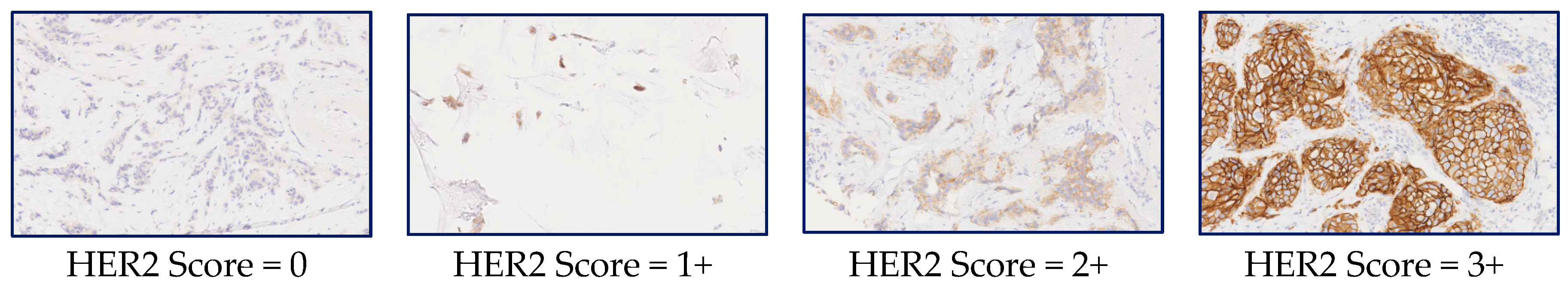
A few sample tiles from WSI images of IHC-stained slides are given in Figure 1 along with the HER2 scores to show the variations of the scores with the level of membrane staining seen in the images.
2.2. Dataset
The dataset used in this research work was provided by the University of Warwick as part of the online HER2 scoring contest [9]. Permission was granted by the contest organizers to participating teams for the use of the dataset for research and academic purposes. The dataset consisted of a total of 172 whole slide images in Nano-zoomer Digital Pathology (NDPI) format. These WSIs were extracted from 86 cases of patients with invasive breast carcinomas [11]. For each case, WSIs of both Hematoxylin and Eosin (H&E)-stained and IHC-stained slides were provided. There were two HER2 scoring contests, and the number of WSIs provided for training and testing the classification algorithm is given in Table 2.
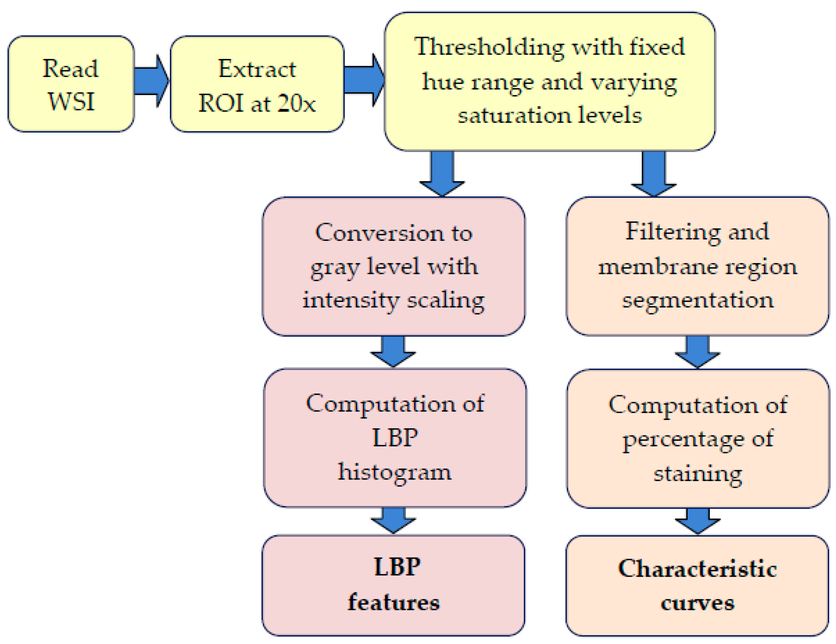
2.3. Processing Stages
Various stages of the processing pipeline are shown in Figure 2. We used the OpenSlide application programming interface (API) [14] to read the WSIs of IHC-stained slides, and a region of interest (ROI) containing a significant portion of the imaged tissue is extracted from the middle segment of the image. Rectangular tiles of size 1800 × 1200 pixels at 20× magnification that contain at most 20% background pixels are then created and used as inputs for the method that computes LBP features and characteristic curves. At least six tiles at randomly selected locations within the ROI are generated for each WSI. The remaining part of the pipeline thresholds the input tiles and computes the LBP features and also the percentage of staining in the tissue sample to obtain the characteristic curves. These steps are detailed in the following sections.
3. Characteristic Curves
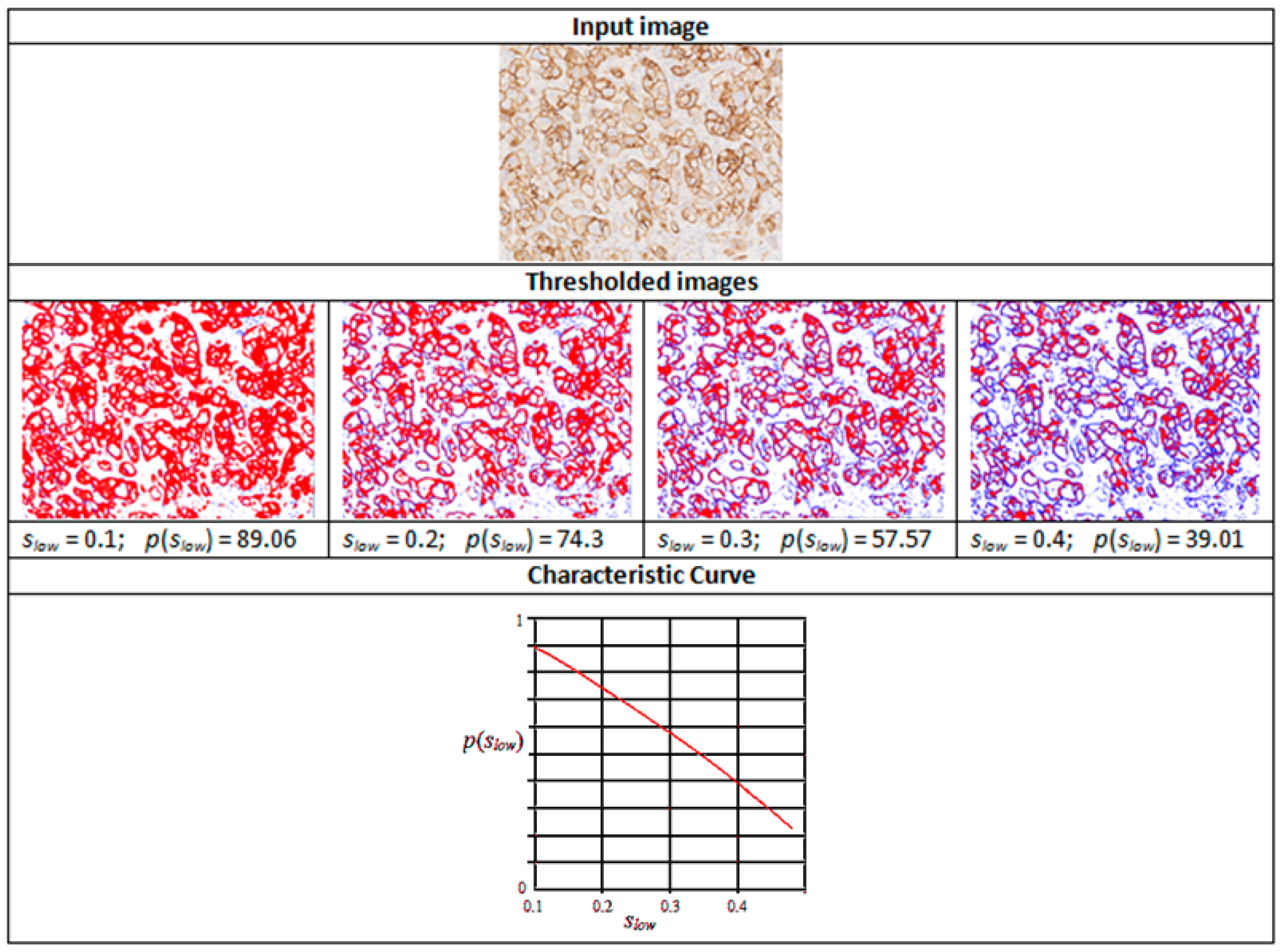
Curve-based automated analysis of immunohistochemical images have been tried in the past with limited success [15]. In this section, we introduce a novel feature vector called a characteristic curve. An important parameter in HER2 assessment is the percentage of membrane staining perceived in an image segment. Assuming that we can compute the percentage of membranes stained in a particular colour range (this computation will be discussed in detail below), we can analyse the variations in this percentage value with respect to changes in the colour saturation threshold. Specifically, if [h, s, v] represent the stain colour components in Hue-Saturation-Value (HSV) space, and if p(slow) denotes the percentage of staining with colour in the range given by the following inequalities:
then, the variation of p(slow) plotted against slow gives the characteristic curve (or the percentage-saturation curve) of the image. In Equation (1), [h1, h2] denote fixed hue thresholds specifying allowable variations in the hue value, and similarly [v1, v2] denote value thresholds. Since we specify only the lower bound for saturation, progressively increasing slow, typically from 0.1 to 0.5, produces a non-increasing characteristic curve (Figure 3). This property of the characteristic curve is the direct result of p(slow) being proportional to the complement of a normalized cumulative histogram for saturation values.
h1 ≤ h < h2
s > slow
v1 ≤ v < v2,
s > slow
v1 ≤ v < v2,
The base components of the stain colour [h, s, v] are computed using the training set where the given percentage of staining is above 80%. While computing the percentage of staining for the test (or cross-validation) sets, it is important to eliminate not only the background region but also other segments that are not part of the membrane region, such as connective tissues, lobules, and nuclei. These regions can be segmented using colour (nuclei are stained in a distinctly different colour) or using a distance measure evaluated in colour space over a neighborhood mask around each pixel (for identifying regions of nearly constant colour value).
Figure 3 shows thresholded images with stained regions in red colour as the value of slow is increased from 0.1 to 0.5. The resulting characteristic curve is also shown. The characteristics curves have the property that they are always monotonically decreasing smooth curves. They allow accurate polynomial approximations using cubic curves. The shape of the curve can be directly matched with the staining patterns given in the HER2 assessment guidelines (Table 1) for a straightforward interpretation of the derived score (Figure 4). For example, the characteristic curve always lies below the 10% threshold when the score is 0, and only a small initial segment of the curve lies above the 10% mark when the score is 1. If the score is 3+, the curve lies completely above the 30% mark, showing a strong and complete membrane staining. As seen in Figure 4, the curve passes through a much wider range of values of percentage staining when the score is 2+.
The properties of the characteristic curve outlined above, particularly the fact that the curve is non-increasing, can be used for developing a naive rule-based classification algorithm as follows.
- If z0 (=p(0.1)) <10%, then the whole curve lies below 10%, and the score is 0
- Else if zn−1 (=p(0.5)) >30%, then the whole curve lies above 30%, and the score is 3+
- Else if 10% ≤ z0 (=p(0.1)) <40% and p(0.2) <15%, the score is 1+
- Else if p(0.4) <15%, then the score is 2+
- Else, the score is 3+
The rules were formed by analyzing the shapes of characteristic curves for several image tiles with ground truth values of HER2 scores assigned by pathologists. Note that for the above simple classification algorithm, we sample the curve at only four key points p(0.1), p(0.2), p(0.4), and p(0.5). We outlined the rule-based algorithm here primarily to show the feature representation capability of the characteristic curves.
4. Local Binary Patterns
4.1. LBP Computation
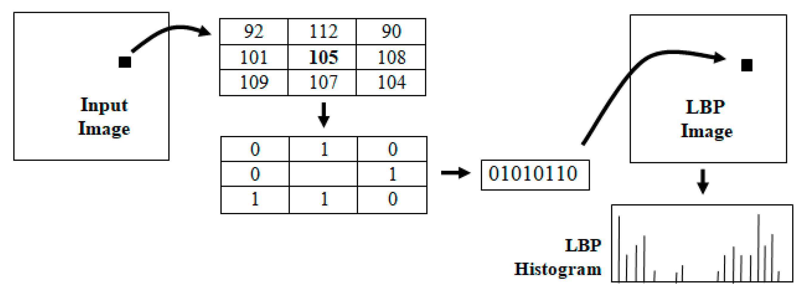
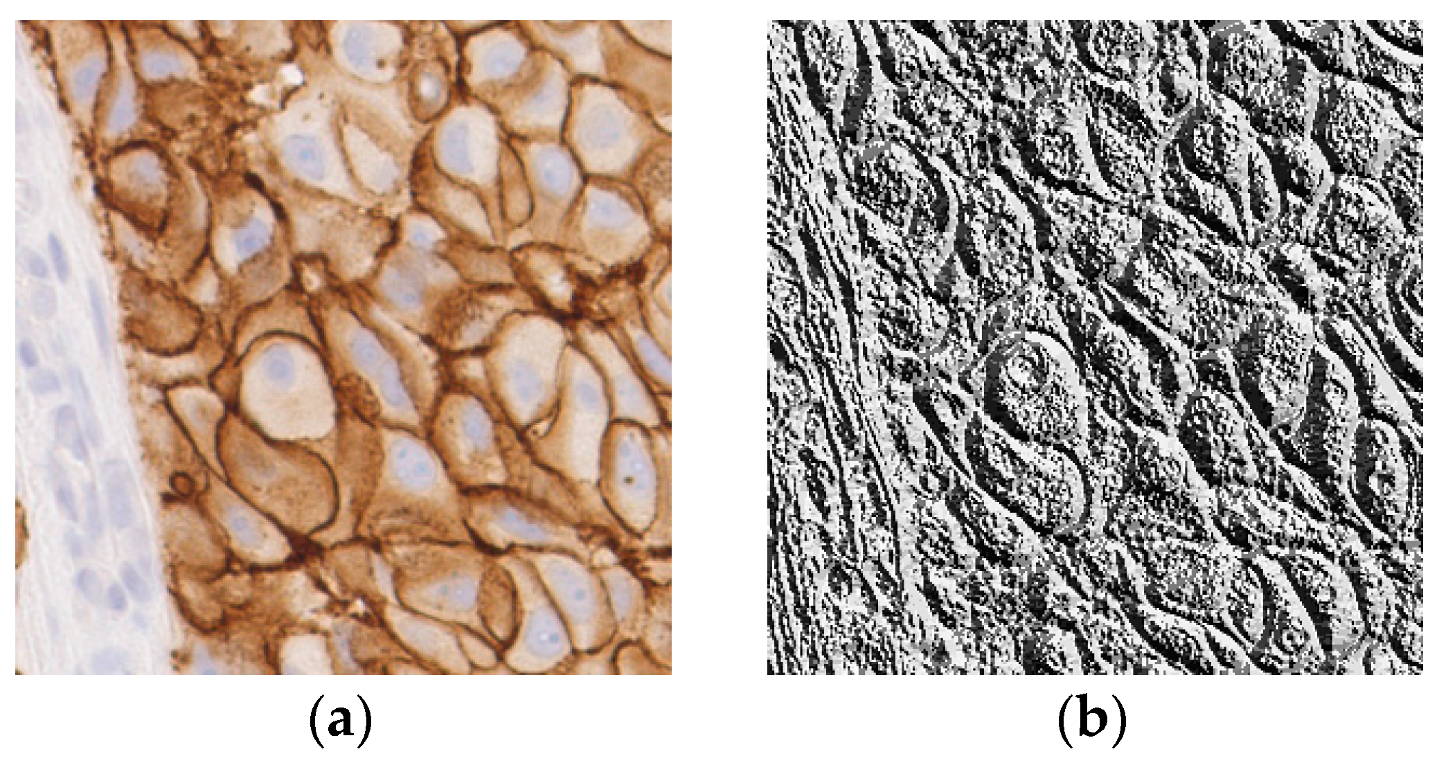
Local binary patterns (LBP) are powerful feature descriptors used for texture analysis and classification [13]. The binary pattern is derived by comparing the intensity at each pixel with its eight neighbors and encoding the information in an 8-bit integer value. This encoding can be viewed as a transformation of the input image into an LBP image as shown in Figure 5. The histogram of the LBP image is generally used for texture classification. In the area of medical image analysis, LBP methods have been successfully used in characterizing disease patterns [16,17,18] and automated diagnosis [19]. Local binary patterns have also been used for analyzing histopathological images and detecting mitotic cells [20,21]. Several variants of LBP features, such as hierarchical LPB, have also been proposed for specific applications, such as retinal vein occlusion recognition [22].
As an example, an input image and its LBP image are shown in Figure 6.
As discussed in Section 3, we first obtain a thresholded image using a hue range [h1, h2] and saturation values with s > slow. The pixels passing the threshold test are converted to gray level by mapping h1 to 0 and h2 to 255. This gray-level image is used as the input for LBP computation. The LBP histogram of such images contain predominant features that represent the texture characteristics of the staining patterns. We denote the 256 values of the LBP histogram by Li, i = 0, …, 255.
4.2. Rotation-Invariant Uniform LBP
Since a region of interest can have any arbitrary orientation, it is important that the extracted features are rotation invariant for consistent results. All image tiles are processed at a fixed magnification of 20×, and therefore it is not necessary to have the scale invariance property. A local binary pattern with at most two bit transitions (0/1 transitions) is referred to as a uniform LBP [23]. Uniform LBPs form predominant texture features in rotation-invariant texture classification algorithms. For LBPs computed using eight neighbours as shown in Figure 5, there are 58 uniform patterns. These patterns can be grouped into nine classes (or types) of uniform local binary patterns (uLBP), depending on the number of 1’s in each pattern, as shown in Table 3. Please note that only those byte values for which the bit pattern contains at most two 0/1 transitions are listed in the table.
Since the byte values of each row in Table 3 contain the same bit pattern circularly shifted among the eight bits, we can obtain a rotation-invariant uLBP by combining the uniform LBPs corresponding to the byte values in each row. The histogram of rotation-invariant uLBP has only nine bins, denoted by Ui, i = 0, …, 8. As an example,
U4 = L15 + L30 + L60 + L120 + L240 + L225 + L195 + L135.
All LBP histogram values corresponding to non-uniform binary patterns are combined into a single bin denoted by Ū:
Ū = L5 + L9 + L10 + + L11 + L13 …
4.3. uLBP Feature Curves
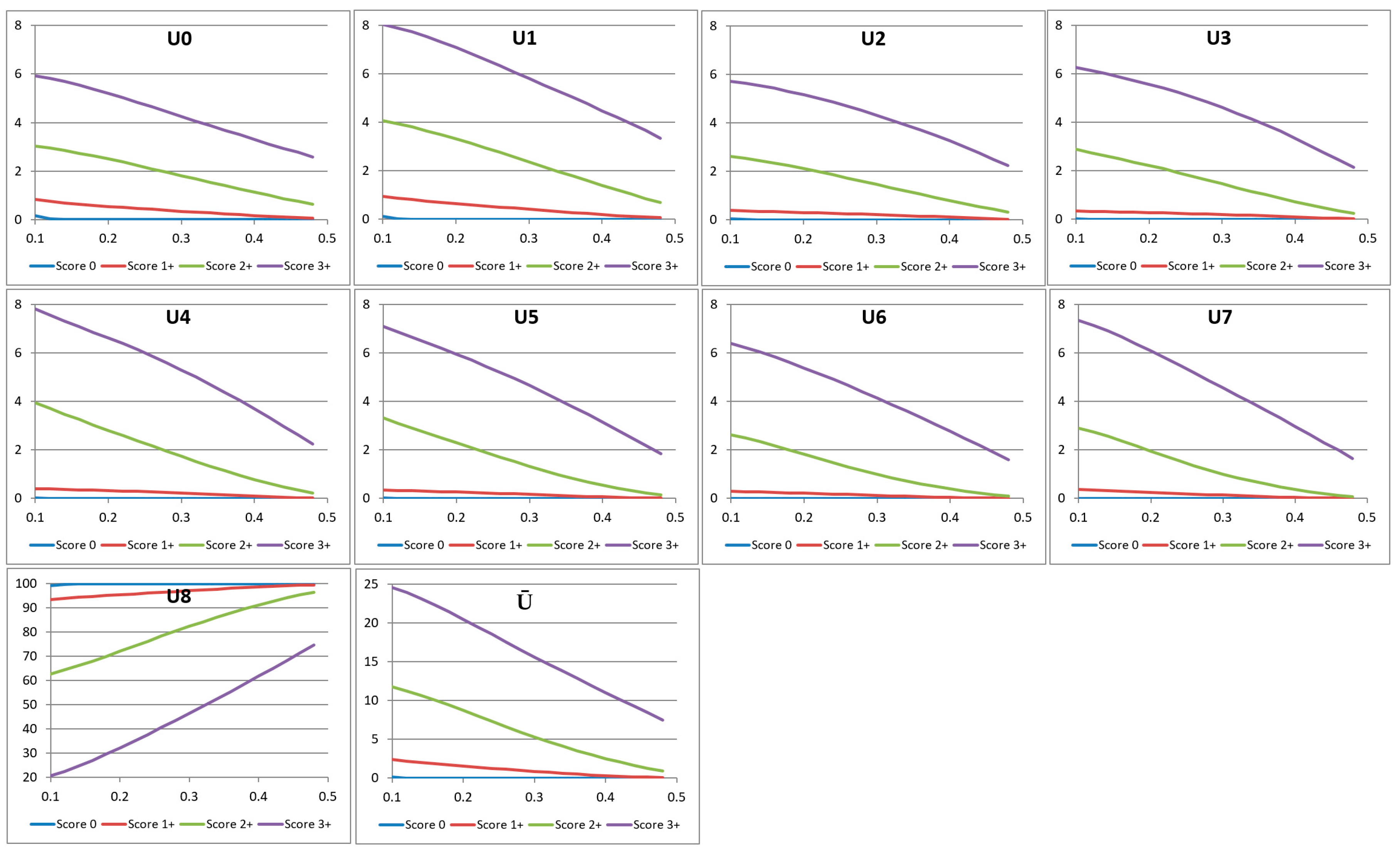
Each of the histogram features Ui in the rotation-invariant uLBP set can generate a feature curve as detailed below. When the input image’s saturation threshold slow is varied from 0.1 to 0.5 as discussed in Section 3, we get the corresponding variation in the LBP values Li. The LBP values are then combined into nine uLBP values Ui as discussed in the previous section. Image regions outside the saturation threshold are assigned a pixel value 0. These “background” pixels of constant intensity will have an LBP value 255, and contribute to the uLBP bin U8. We discard the value of U8, as it mainly represents regions of constant intensity. The variation in the values of the remaining bins Ui, i = 0, …, 7 shows a non-increasing trend very similar to that of the characteristic curve (Figure 7).
The values of the uLBP feature curves are converted to percentages to remove any variations due to changes in image size as follows:
where, w and h denote the width and the height of the input image, respectively. The variations of the uLBP feature components Ui, i = 0, …, 8 and also the non-uniform component Ū for images with HER2 scores 0, 1+, 2+, and 3+ are shown in Figure 7.
Ui′ = Ui·100/(w·h)
The uLBP feature curves bear similarity with characteristic curves in that they do not contain high frequency variations and are non-increasing. Further, as can be seen in Figure 7, uLBP feature curves Ui, i = 0, …, 7 show excellent discriminating power between the four HER2 classes, making them highly suitable for use as feature vectors in HER2 classification algorithms.
5. HER2 Classification and Scoring
In this section, we outline a ‘one-vs-all’ multi-class classification algorithm using logistic regression [24]. Logistic regression was chosen to minimize the computational complexity. Higher-order methods, such as neural networks, could also be designed with the use of the feature vectors proposed in this paper. For a given training example with index j, the points sampled along its characteristic curve or LBP feature curve xi(j) = p(si), i = 1, …, n, j = 1, …, m are used as features. The class labels are denoted by yj ∈ [0, 3], j = 1, …, m. We denote the feature matrix by X ∈ ℜm×(n+1), the output vector of labels by Y ∈ ℜm×1, and the classifier parameter vector for each class by θk ∈ ℜ(n+1)×1, k = 1, …, 4. Here, class-1 corresponds to the set of training examples with HER2 score 1+, class-2 with HER2 score 2+, class-3 with HER2 score 3+, and class-4 with HER2 score 0. We then have the following equations for the hypothesis functions H, the cost function, and the gradient functions:
where, H ∈ ℜm×1, and g() denotes the sigmoid function. The cost function J(θk) is then given by
and the gradient function vector J′(θk) is defined as
H = g(Xθk)
For prediction, the points xi on the characteristic curve or the LBP feature curve of a given sample are combined with the trained values of class parameters θk for each class k = 1, …, 4, and the class that gives the maximum value for g(xi′θk) is chosen. In the next section, we provide the result of classification experiments using the above methods.
6. Experimental Results and Analysis
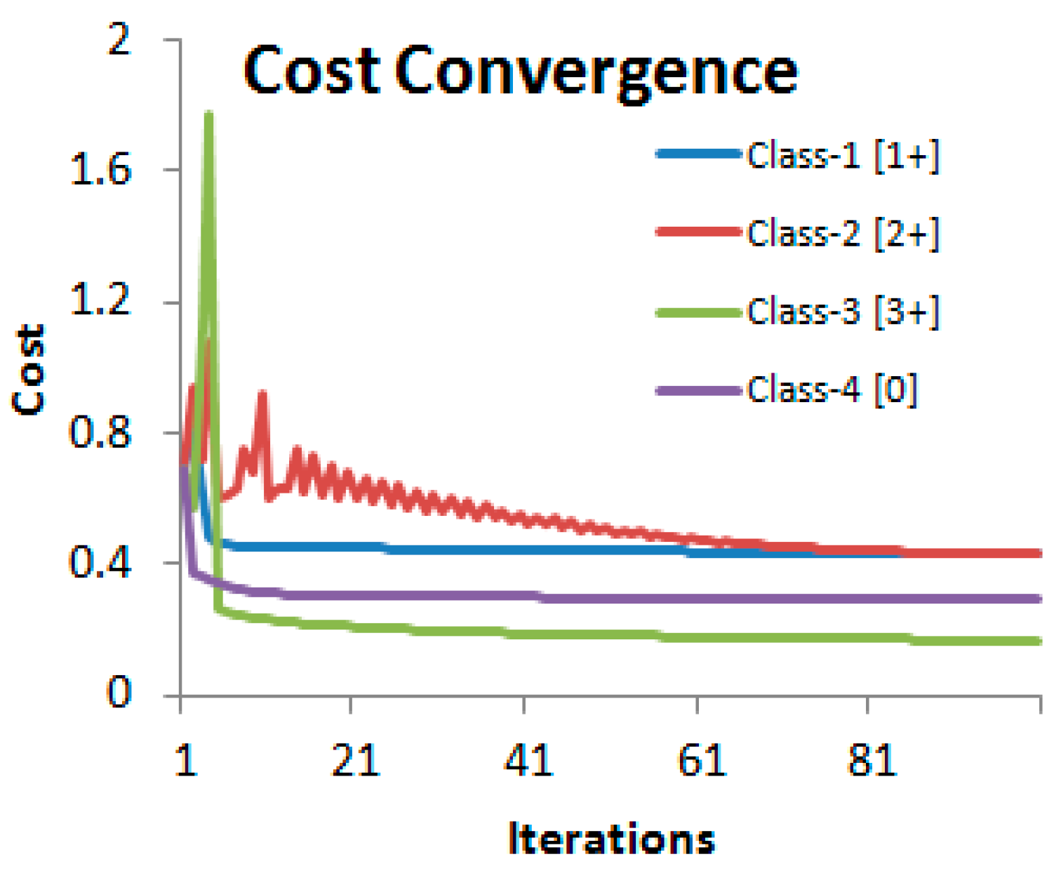
We used features computed from 52 WSIs with 3 tiles at 20× from each image (comprising of 156 images) and their ground truth values as the training data. Another set of 3 tiles from each of the 52 cases formed the cross-validation set. Out of the total of 156 image tiles in the cross-validation set, 39 belonged to each of the four classes corresponding to four HER2 scores. For generating feature vectors for classification using logistic regression, it was found that a step size of 0.02 for the saturation threshold would provide an adequate number of 20 points (features) within the saturation range slow ∈ [0.1, 0.5]. The feature matrix X in Equation (5) therefore had the dimension 156 × 20. The gradient descent algorithm used 100 iterations to converge to the solution with a learning rate of 0.001 (Figure 8).
The confusion matrix in Table 4 summarizes the results for each class and gives the overall accuracy achieved.
The smoothness and monotonically decreasing properties of the characteristic curve can be effectively made use of in reducing the dimensionality of the features in the logistic regression algorithm. As in the case of the rule-based classification method, we can sample the curve at only four key points p(0.1), p(0.2), p(0.4), and p(0.5), and also use the slope information at those points p′(0.1), p′(0.2), p′(0.4), and p′(0.5) to get a feature vector of size 8 instead of 20. The cost functions converge to almost similar values with only a slight increase in the magnitudes. The confusion matrix obtained by running the algorithm with the reduced set of features of the characteristic curve is shown in Table 5.
As seen in Table 5, reducing the dimensionality of the feature set from 20 to 8 only affected the recall rates of classes 1 and 2.
An experimental analysis using uLBP feature curves also gave good levels of accuracy. Only the first eigtht uLBP feature curves Ui, i = 0, …, 7, each containing 20 sample points, were used in our analysis. We give below the classification results as a confusion matrix (Table 6).
The texture characteristics represented by uLBP features were useful in resolving some of the ambiguous cases for scores 0 and 3+ where the texture features are highly distinguishable, providing higher recall rates for those two scores. The uLBP features also gave higher false positives for score 2+.
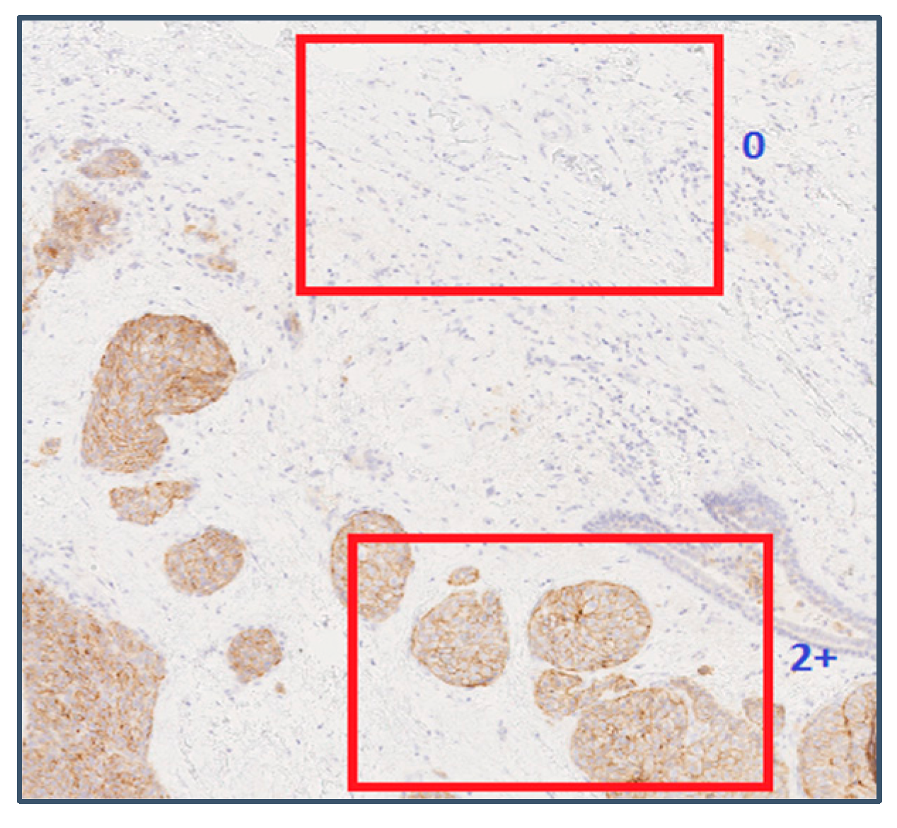
Analysing the staining patterns in tiles that were wrongly classified revealed a common problem in the automatic extraction of tiles from WSIs. Some of the samples with scores 1+ and 2+ had large tissue regions without any staining. The example shown in Figure 9 contains a tissue sample at 10× magnification with an assigned score of 2+.
In Figure 9, the tile on the top did not contain any stained membrane regions, and was assigned a ground truth value of 2+ at the training stage and a predicted value of 0 at the cross-validation stage. This tile could have been a valid part of any WSI with a score 0, and therefore there is no way by which such tiles can be identified and discarded by the automatic tile extraction method. Manually identifying such tiles from the training and cross-validation sets significantly improved the scores of the classification algorithms. The tile on the bottom half of Figure 9 was assigned the correct score of 2+.
7. Conclusions and Future Work
This paper has introduced two novel feature descriptors viz. characteristic curves and LBP feature curves that could be effectively used in classification algorithms for the automated scoring of HER2 in breast cancer histology slides. The computational aspects of both types of descriptors and their shape feature representation capabilities in embedding information about the staining patterns and the percentage of staining present in images with different HER2 scores have been discussed in detail. Both descriptors have similar geometrical attributes in that they are both smooth non-increasing curves. Experimental analyses have shown that both descriptors have excellent interclass variance and intraclass correlation properties that make them useful for applications in classification algorithms. Results of an experimental analysis done using a comprehensive WSI dataset provided by the University of Warwick [9] has also been presented. The results show that the features used with a multi-class classification algorithm, such as logistic regression, can provide very good levels of accuracy. The paper also outlined computational stages in the overall processing pipeline for automatic HER2 scoring using WSI files as inputs.
Experimental results given in the paper also show the need for further improving the discriminating power of the features. Further analysis is required for the accurate identification of membrane morphology and region segmentation, particularly for samples with an assigned HER2 score 1+. It is also necessary to assess the reproducibility of results, specifically the inter-scanner variability [25] of the rule-based classification algorithm, as the rules were formed using data produced by a single scanner. Future work is also directed towards graphical processing unit (GPU) implementations of the feature extraction methods.
Acknowledgments
All sources of funding of the study should be disclosed. Please clearly indicate grants that you have received in support of your research work. Clearly state if you received funds for covering the costs to publish in open access.
Conflicts of Interest
The author declares no conflict of interest.
References
- Hicks, D.G.; Schiffhauer, L. Standardized assessment of the Her2 status in breast cancer by immunohistochemistry. Lab. Med. 2015, 42, 459–467. [Google Scholar] [CrossRef]
- Rakha, E.A.; Pinder, S.E.; Bartlett, J.M.; Ibrahim, M.; Starczynski, J.; Carder, P.J.; Provenzano, E.; Hanby, A.; Hales, S.; Lee, A.H.; et al. Updated UK recommendations for HER2 assessment in breast cancer. J. Clin. Pathol. 2015, 68, 93–99. [Google Scholar] [CrossRef] [PubMed] [Green Version]
- Gavrielides, M.A.; Gallas, B.D.; Lenz, P.; Badano, A.; Hewitt, S.M. Observer variability in the interpretation of HER2 immunohistochemical expression with unaided and computer aided digital microscopy. Arch. Pathol. Lab. Med. 2011, 135, 233–242. [Google Scholar] [CrossRef] [PubMed]
- Akbar, S.; Jordan, L.B.; Purdie, C.A.; Thompson, A.M.; McKenna, S.J. Comparing computer-generated and pathologist-generated tumour segmentations for immunohistochemical scoring of breast tissue microarrays. Br. J. Cancer 2015, 113, 1075–1080. [Google Scholar] [CrossRef] [PubMed] [Green Version]
- Hamilton, P.W.; Bankhead, P.; Wang, Y.; Hutchinson, R.; Kieran, D.; McArt, D.G.; James, J.; Salto-Tellez, M. Digital pathology and image analysis in tissue biomarker research. Methods 2014, 70, 59–73. [Google Scholar] [CrossRef] [PubMed]
- Farahani, N.; Parwani, A.V.; Pantanowitz, L. Whole slide imaging in pathology: Advantages, limitations and emerging perspectives. Pathol. Lab. Med. Int. 2015, 7, 23–33. [Google Scholar] [CrossRef]
- Ghaznavi, F.; Evan, A.; Madabhushi, A.; Feldman, M. Digital imaging in pathology: Whole-slide imaging and beyond. Annu. Rev. Pathol. Mech. Dis. 2013, 8, 31–59. [Google Scholar] [CrossRef] [PubMed]
- Razavi, S.; Hatipoglu, G.; Yalcin, H. Automatically diagnosing HER2 amplification status for breast cancer patients using large FISH images. In Proceedings of the 25th Signal Processing and Communications Applications Conference, Antalya, Turkey, 15–18 May 2017; pp. 1–4. [Google Scholar]
- Department of Computer Science, University of Warwick: Her2 Scoring Contest. Available online: http://www2.warwick.ac.uk/fac/sci/dcs/research/combi/research/bic/her2contest/ (accessed on 15 November 2016).
- Department of Computer Science, University of Warwick: Her2 Contest Results. Available online: http://www2.warwick.ac.uk/fac/sci/dcs/research/combi/research/bic/her2contest/outcome (accessed on 15 November 2016).
- Qaiser, T.; Mukherjee, A.; Reddy Pb, C.; Munugoti, S.D.; Tallam, V.; Pitkäaho, T.; Lehtimäki, T.; Naughton, T.; Berseth, M.; Pedraza, A.; et al. Her2 Challenge Contest: A detailed assessment of Her2 scoring algorithms and man vs machine in whole slide images of breast cancer tissues. Histopathology 2018, 72, 227–238. [Google Scholar] [CrossRef] [PubMed]
- Mukundan, R. A Robust Algorithm for Automated Her2 Scoring in Breast Cancer Histology Slides Using Characteristic Curves. In Medical Image Understanding and Analysis; Communications in Computer and Information Science; Valdés Hernández, M., González-Castro, V., Eds.; Springer: Cham, Switzerland, 2017; Volume 723, pp. 386–397. [Google Scholar]
- Pietikainen, M.; Zhao, G.; Hadid, A.; Ahonen, T. Computer Vision Using Local Binary Patterns; Springer: London, UK, 2011; ISBN 978-0-85729-748-8. [Google Scholar]
- Goode, A.; Gilbert, B.; Harkes, J.; Jukie, D.; Satyanarayanan, M. OpenSlide: A vendor-neutral software foundation for digital pathology. J. Pathol. Inform. 2013, 4. [Google Scholar] [CrossRef]
- Livanos, G.; Zervakis, M.; Giakos, G.C. Automated analysis of immunohistochemical images based on curve evolution approaches. In Proceedings of the IEEE Conference of Imaging Systems and Techniques, Beijing, China, 22–23 October 2013; pp. 112–115. [Google Scholar]
- Sørensen, L.; Shaker, S.B.; de Bruijne, M. Quantitative analysis of pulmonary emphysema using local binary patterns. IEEE Trans. Med. Imaging 2010, 29, 559–569. [Google Scholar] [CrossRef] [PubMed]
- Morales, S.; Engan, K.; Naranjo, V.; Colomer, A. Detection of diabetic retinopathy and age-related macular degeneration from fundus images through local binary patterns and random forests. In Proceedings of the IEEE International Conference on Image Processing, Quebec City, QC, Canada, 27–30 September 2015; pp. 4838–4842. [Google Scholar]
- Sarwinda, D.; Bustamam, A. Detection of Alzheimer’s disease using advanced local binary pattern from hippocampus and whole brain of MR images. In Proceedings of the International Joint Conference on Neural Networks, Vancouver, BC, Canada, 24–29 July 2016; pp. 5051–5056. [Google Scholar]
- Tiwari, A.K.; Pachori, R.B.; Kanhangad, V.; Panigrahi, B.K. Automated diagnosis of epilepsy using key-point based local binary pattern of EEG signals. IEEE J. Biomed. Health Inform. 2017, 21, 888–896. [Google Scholar] [CrossRef] [PubMed]
- Urdal, J.; Engan, K.; Kvikstad, V.; Janssen, E.A.M. Prognostic prediction of histopathological images by local binary patterns and RUSBoost. In Proceedings of the 25th European Signal Processing Conference, Kos, Greece, 2 September 2017; pp. 2349–2353. [Google Scholar]
- Sigirci, I.O.; Albayrak, A.; Bilgin, G. Detection of mitotic cells using completed local binary pattern in histopathological images. In Proceedings of the 23rd Signal Processing and Communications Applications Conference, Malatya, Turkey, 16–19 May 2015; pp. 1078–1081. [Google Scholar]
- Zhang, H.; Chen, Z.; Chi, Z.; Fu, H. Hierarchical local binary pattern for branch retinal vein occlusion recognition with fluorescein angiography images. Electron. Lett. 2014, 50, 1902–1904. [Google Scholar] [CrossRef]
- Ojala, T.; Pietikainen, M.; Maenpaa, T. Multiresolution gray-scale and rotation invariant texture classification with local binary patterns. IEEE Trans. Pattern Anal. Mach. Intell. 2002, 24, 971–987. [Google Scholar] [CrossRef]
- Watt, J.; Borhani, R.; Katsaggelos, A.K. Machine Learning Refined: Foundations, Algorithms and Applications, 1st ed.; Cambridge Uniersity Press: Cambridge, UK, 2016; ISBN 978-1107123526. [Google Scholar]
- Keay, T.; Conway, C.M.; O’Flaherty, N.; Hewitt, S.M.; Shea, K.; Gavrielides, M.A. Reproducibility in the automated quantitative assessment of HER2/neu for breast cancer. J. Pathol. Inform. 2013, 4. [Google Scholar] [CrossRef]
Figure 1.
Whole Slide Image (WSI) tiles showing different levels of staining and their corresponding HER2 scores. Reproduced from [12] with permission.
Figure 1.
Whole Slide Image (WSI) tiles showing different levels of staining and their corresponding HER2 scores. Reproduced from [12] with permission.

Figure 2.
Processing stages in the extraction of characteristic curves and local binary pattern (LBP) features. ROI: region of interest.
Figure 2.
Processing stages in the extraction of characteristic curves and local binary pattern (LBP) features. ROI: region of interest.

Figure 3.
Intermediate stages in the generation of a characteristic curve. Reproduced from [12] with permission.
Figure 3.
Intermediate stages in the generation of a characteristic curve. Reproduced from [12] with permission.

Figure 4.
Variations in the shapes of the characteristic curves with different levels of staining. Reproduced from [12] with permission.
Figure 4.
Variations in the shapes of the characteristic curves with different levels of staining. Reproduced from [12] with permission.

Figure 5.
The intermediate steps in the computation of the LBP histogram of an image.

Figure 6.
(a) A sample input image for LBP computation; (b) The corresponding LBP image.

Figure 7.
The values of the first four uniform local binary pattern (uLBP) bins corresponding to four images with different HER2 scores. The x-axis denotes the variation of the saturation threshold slow from 0.1 to 0.5.
Figure 7.
The values of the first four uniform local binary pattern (uLBP) bins corresponding to four images with different HER2 scores. The x-axis denotes the variation of the saturation threshold slow from 0.1 to 0.5.

Figure 8.
Convergence of the cost functions of the four-class logistic regression algorithm. Reproduced from [12] with permission.
Figure 8.
Convergence of the cost functions of the four-class logistic regression algorithm. Reproduced from [12] with permission.

Figure 9.
An example showing two tile positions with varying image characteristics within the same WSI. Reproduced from [12] with permission.
Figure 9.
An example showing two tile positions with varying image characteristics within the same WSI. Reproduced from [12] with permission.


Table 1.
Correlation between the intensity and percentage of membrane staining and the assigned HER2 scores [2]. Reproduced from [12] with permission.
| HER2 Score | Assessment | Staining Pattern |
|---|---|---|
| 0 | Negative | No staining is observed, or membrane staining is observed in less than 10% of tumor cells |
| 1+ | Negative | A faint/barely perceptible membrane staining is detected in greater than 10% of tumor cells. The cells exhibit incomplete membrane staining. |
| 2+ | Weakly Positive | A weak to moderate membrane staining is observed in greater than 10% of tumor cells. |
| 3+ | Positive | A strong complete membrane staining is observed in greater than 10% of tumor cells. |
Table 2.
Number of WSIs provided for training and testing the classification algorithm. Reproduced from [12] with permission.
Table 2.
Number of WSIs provided for training and testing the classification algorithm. Reproduced from [12] with permission.
| Training Set | Test Set | ||
|---|---|---|---|
| Ground Truth HER2 Score | Number of WSIs | Contest-1 No. of WSIs | Contest-2 No. of WSIs |
| 0 | 13 | 28 | 6 |
| 1+ | 13 | ||
| 2+ | 13 | ||
| 3+ | 13 | ||
| Total | 52 | ||
Table 3.
Nine different classes of uniform Local Binary Patterns.
| Number of 1’s | Byte Values | |||||||
|---|---|---|---|---|---|---|---|---|
| 0 | 0 | |||||||
| 1 | 1 | 2 | 4 | 8 | 16 | 32 | 64 | 128 |
| 2 | 3 | 6 | 12 | 24 | 48 | 96 | 192 | 129 |
| 3 | 7 | 14 | 28 | 56 | 112 | 224 | 193 | 131 |
| 4 | 15 | 30 | 60 | 120 | 240 | 225 | 195 | 135 |
| 5 | 31 | 62 | 124 | 248 | 241 | 227 | 199 | 143 |
| 6 | 63 | 126 | 252 | 249 | 243 | 231 | 207 | 159 |
| 7 | 127 | 254 | 253 | 251 | 247 | 239 | 223 | 191 |
| 8 | 255 | |||||||
Table 4.
Confusion matrix for the multi-class logistic regression algorithm. Reproduced from [12] with permission.
Table 4.
Confusion matrix for the multi-class logistic regression algorithm. Reproduced from [12] with permission.
| HER2 Score | Predicted | Accuracy = 88.46% | |||||
|---|---|---|---|---|---|---|---|
| 0 | 1+ | 2+ | 3+ | Precision | Recall | ||
| Actual | 0 | 37 | 2 | 0 | 0 | 0.86 | 0.95 |
| 1+ | 6 | 29 | 4 | 0 | 0.83 | 0.74 | |
| 2+ | 0 | 4 | 34 | 1 | 0.87 | 0.87 | |
| 3+ | 0 | 0 | 1 | 38 | 0.97 | 0.97 | |
Table 5.
Confusion matrix for the multi-class logistic regression algorithm with the reduced feature set. Reproduced from [12] with permission.
Table 5.
Confusion matrix for the multi-class logistic regression algorithm with the reduced feature set. Reproduced from [12] with permission.
| HER2 Score | Predicted | Accuracy = 83.3% | |||||
|---|---|---|---|---|---|---|---|
| 0 | 1+ | 2+ | 3+ | Precision | Recall | ||
| Actual | 0 | 37 | 2 | 0 | 0 | 0.80 | 0.95 |
| 1+ | 8 | 24 | 7 | 0 | 0.75 | 0.61 | |
| 2+ | 1 | 6 | 31 | 1 | 0.79 | 0.79 | |
| 3+ | 0 | 0 | 1 | 38 | 0.97 | 0.97 | |
Table 6.
Confusion matrix for the multi-class logistic regression algorithm with uLBP feature vectors.
Table 6.
Confusion matrix for the multi-class logistic regression algorithm with uLBP feature vectors.
| HER2 Score | Predicted | Accuracy = 90.38% | |||||
|---|---|---|---|---|---|---|---|
| 0 | 1+ | 2+ | 3+ | Precision | Recall | ||
| Actual | 0 | 38 | 1 | 0 | 0 | 0.86 | 0.97 |
| 1+ | 5 | 31 | 3 | 0 | 0.86 | 0.79 | |
| 2+ | 1 | 4 | 33 | 1 | 0.92 | 0.85 | |
| 3+ | 0 | 0 | 0 | 39 | 0.98 | 1.00 | |
© 2018 by the author. Licensee MDPI, Basel, Switzerland. This article is an open access article distributed under the terms and conditions of the Creative Commons Attribution (CC BY) license (http://creativecommons.org/licenses/by/4.0/).
Share and Cite
MDPI and ACS Style
Mukundan, R. Image Features Based on Characteristic Curves and Local Binary Patterns for Automated HER2 Scoring. J. Imaging 2018, 4, 35. https://0-doi-org.brum.beds.ac.uk/10.3390/jimaging4020035
AMA Style
Mukundan R. Image Features Based on Characteristic Curves and Local Binary Patterns for Automated HER2 Scoring. Journal of Imaging. 2018; 4(2):35. https://0-doi-org.brum.beds.ac.uk/10.3390/jimaging4020035
Chicago/Turabian StyleMukundan, Ramakrishnan. 2018. "Image Features Based on Characteristic Curves and Local Binary Patterns for Automated HER2 Scoring" Journal of Imaging 4, no. 2: 35. https://0-doi-org.brum.beds.ac.uk/10.3390/jimaging4020035
Note that from the first issue of 2016, this journal uses article numbers instead of page numbers. See further details here.