Lensless Three-Dimensional Quantitative Phase Imaging Using Phase Retrieval Algorithm

 ,
,
Abstract
:1. Introduction
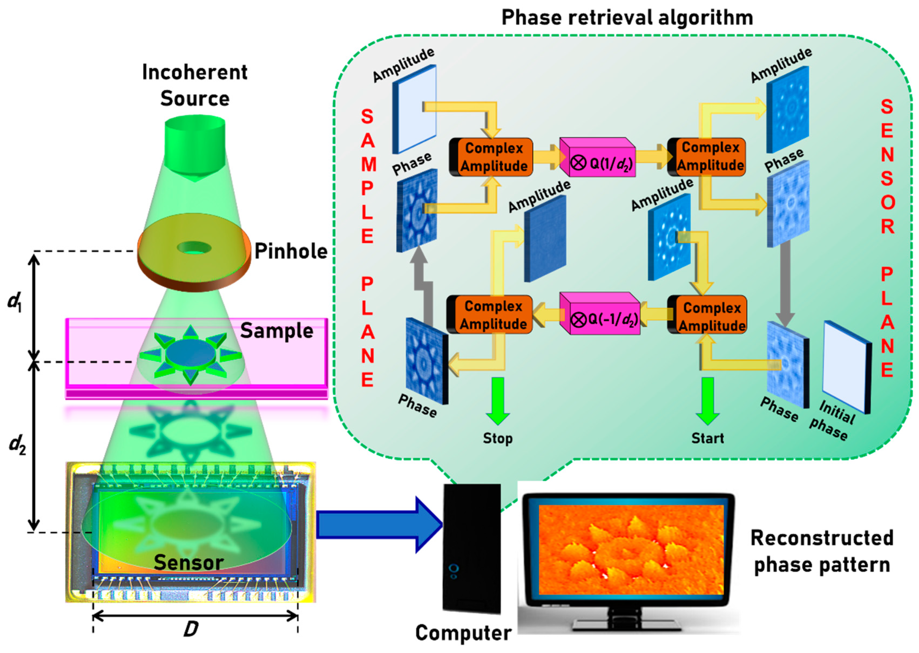
2. Methodology
3. Computational Procedure
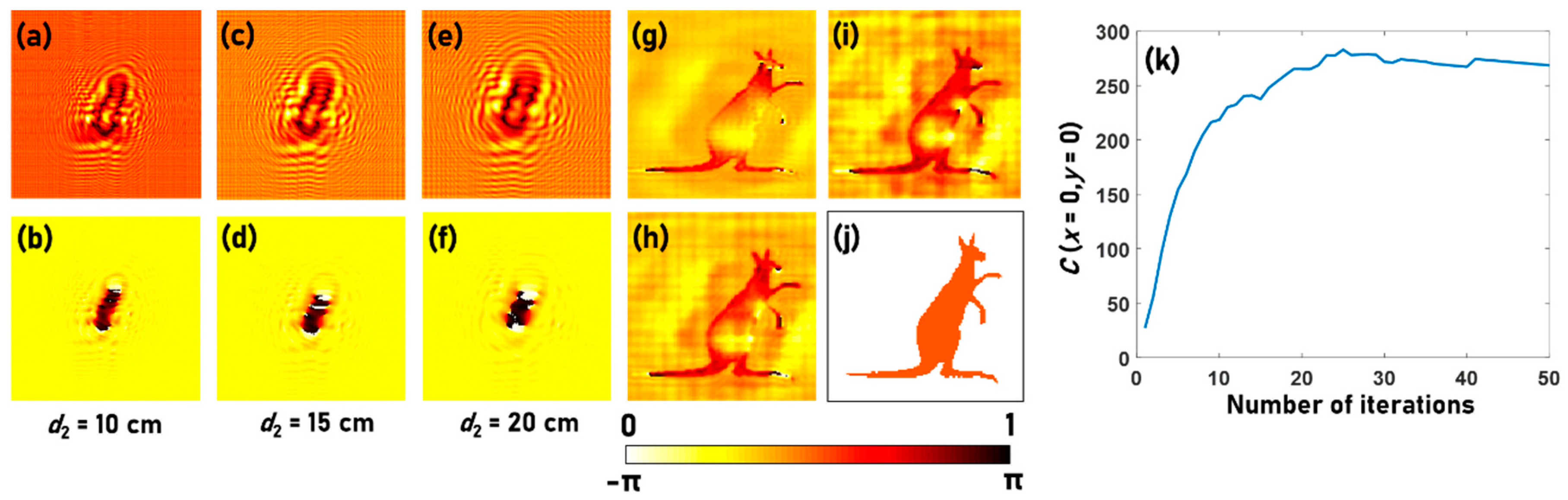
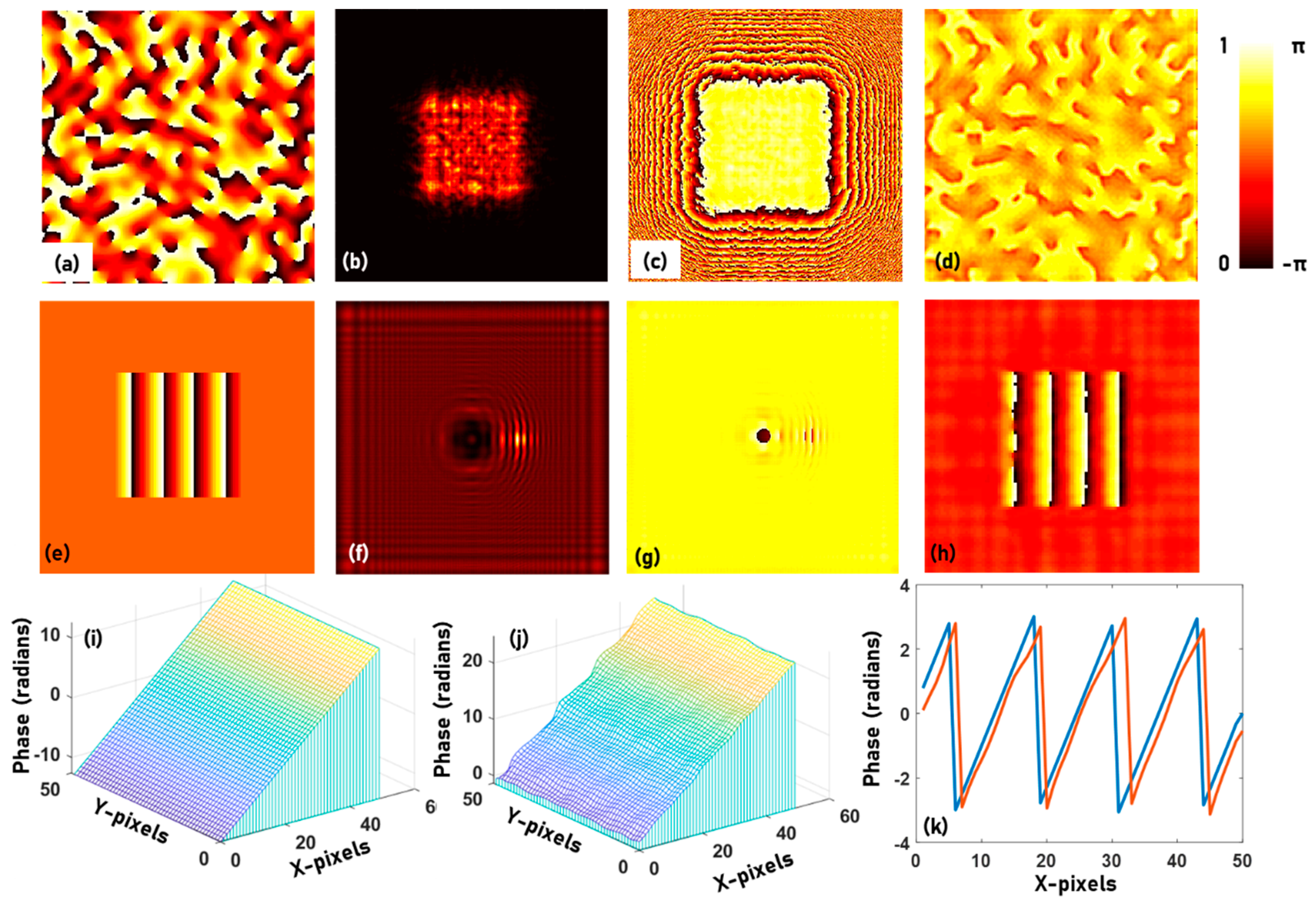
4. Simulative Studies
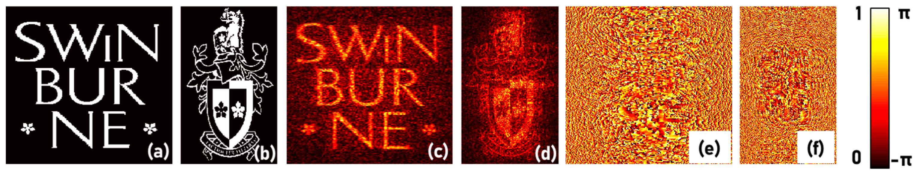
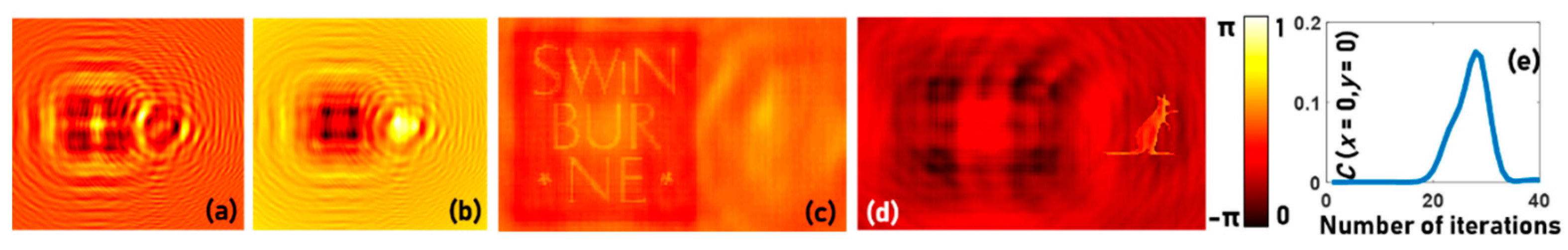
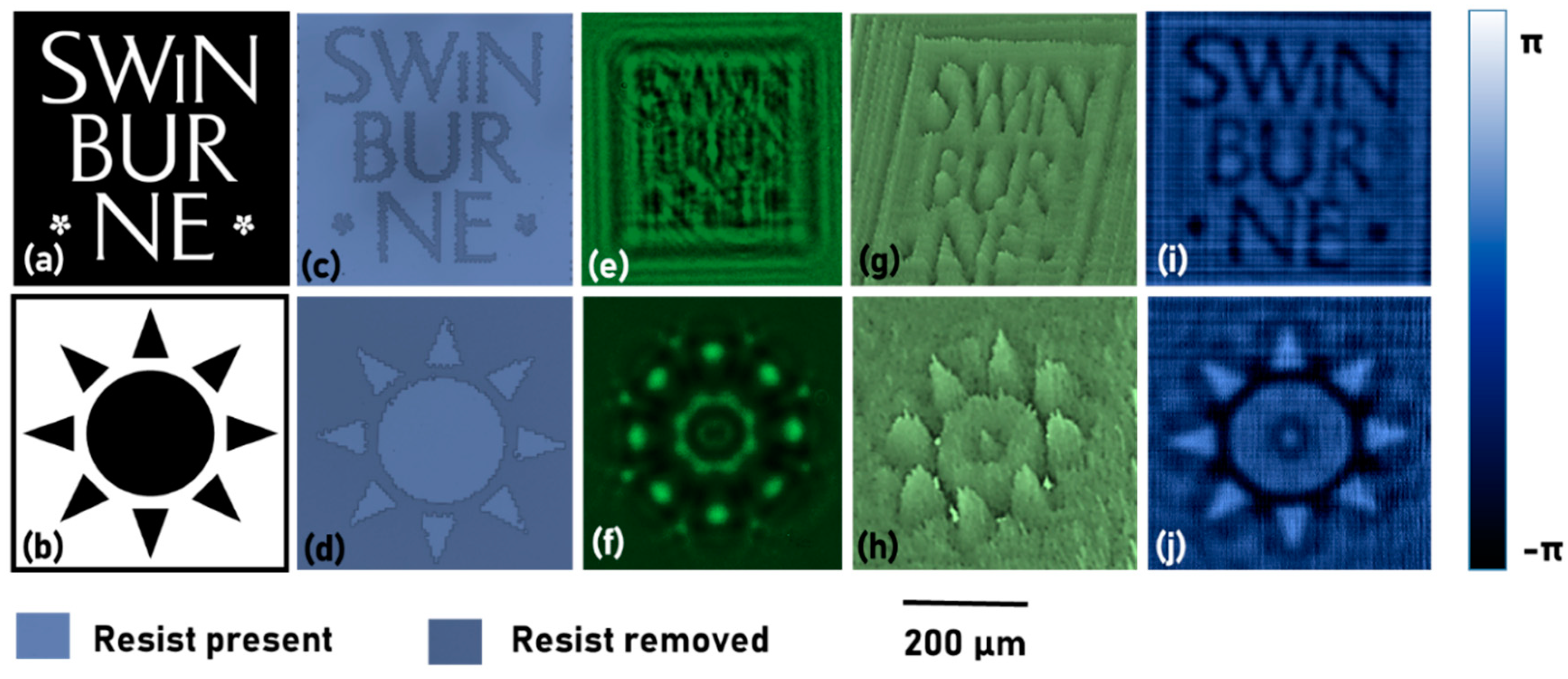
5. Experiments and Results
6. Discussion
7. Summary, Conclusions, Outlook
Supplementary Materials
Author Contributions
Funding
Acknowledgments
Conflicts of Interest
References
- Ross, K.F.A. Phase Contrast and Interference Microscopy for Cell Biologists; Edward Arnold: London, UK, 1967. [Google Scholar]
- Popescu, G. Quantitative Phase Imaging of Cells and Tissues; McGraw-Hill: New York, NY, USA, 2011. [Google Scholar]
- Park, Y.; Depeursinge, C.; Popescu, G. Quantitative phase imaging in biomedicine. Nat. Photonics 2018, 12, 578–589. [Google Scholar] [CrossRef]
- Tsuruta, T.; Itoh, Y. Hologram Schlieren and phase-contrast methods. Jpn. J. Appl. Phys. 1969, 8, 96–103. [Google Scholar] [CrossRef]
- Zernike, F. Phase-contrast, a new method for microscopic observation of transparent objects. Part II. Physica 1942, 9, 974–986. [Google Scholar] [CrossRef]
- Barty, A.; Nugent, K.A.; Roberts, A.; Paganin, D. Quantitative phase tomography. Opt. Commun. 2000, 175, 329–336. [Google Scholar] [CrossRef]
- Lebedeff, A.A. L’interféromètre à polarisation et ses applications. Rev. Opt. 1930, 9, 385–413. [Google Scholar]
- Françon, M. Polarization Interference Microscopes. Appl. Opt. 1964, 3, 1033–1036. [Google Scholar] [CrossRef]
- Koester, C.J.; Osterberg, H.; Willman, H.E. Transmittance Measurements with an Interference Microscope. J. Opt. Soc. Am. 1960, 50, 477–482. [Google Scholar] [CrossRef]
- Kreis, T. Digital holographic interference-phase measurement using the Fourier-transform method. J. Opt. Soc. Am. A. 1986, 3, 847–855. [Google Scholar] [CrossRef]
- Gleyzes, P.; Boccara, A.C.; Saint-Jalmes, H. Multichannel Nomarskimicroscope with polarization modulation: Performance and applications. Opt. Lett. 1997, 22, 1529–1531. [Google Scholar] [CrossRef]
- Totzeck, M.; Tiziani, H.J. Phase-shifting polarization interferometry for microstructure linewidth measurement. Opt. Lett. 1999, 24, 294–296. [Google Scholar] [CrossRef]
- Cuche, E.; Bevilacqua, F.; Depeursinge, C. Digital holography for quantitative phase-contrast imaging. Opt. Lett. 1999, 24, 291–293. [Google Scholar] [CrossRef] [PubMed]
- Machikhin, A.; Polschikova, O.; Ramazanova, A.; Pozhar, V. Multi-spectral quantitative phase imaging based on filtration of light via ultrasonic wave. J. Opt. 2017, 19, 075301. [Google Scholar] [CrossRef]
- Kumar, M.; Quan, X.; Awatsuji, Y.; Tamada, Y.; Matoba, O. Digital Holographic Multimodal Cross-Sectional Fluorescence and Quantitative Phase Imaging System. Sci. Rep. 2020, 10, 7580. [Google Scholar] [CrossRef] [PubMed]
- Shaked, N.T.; Rinehart, M.T.; Wax, A. Dual-interference-channel quantitative-phase microscopy of live cell dynamics. Opt. Lett. 2009, 34, 767–769. [Google Scholar] [CrossRef] [Green Version]
- Hai, N.; Rosen, J. Interferenceless and motionless method for recording digital holograms of coherently illuminated 3-D objects by coded aperture correlation holography system. Opt. Express 2019, 27, 24324–24339. [Google Scholar] [CrossRef] [PubMed]
- Hai, N.; Rosen, J. Doubling the acquisition rate by spatial multiplexing of holograms in coherent sparse coded aperture correlation holography. Opt. Lett. 2020, 45, 3439–3442. [Google Scholar] [CrossRef] [PubMed]
- Chhaniwal, V.; Singh, A.S.G.; Leitgeb, R.A.; Javidi, B.; Anand, A. Quantitative phase-contrast imaging with compact digital holographic microscope employing Lloyd’s mirror. Opt. Lett. 2012, 37, 5127–5129. [Google Scholar] [CrossRef]
- Girshovitz, P.; Shaked, N.T. Compact and portable low-coherence interferometer with off-axis geometry for quantitative phase microscopy and nanoscopy. Opt. Express 2013, 21, 5701–5714. [Google Scholar] [CrossRef]
- Zhang, Y.; Pedrini, G.; Osten, W.; Tiziani, H.J. Phase retrieval microscopy for quantitative phase-contrast imaging. Optik 2004, 115, 94–96. [Google Scholar] [CrossRef]
- Gerchberg, R.W.; Saxton, W.O. A practical algorithm for the determination of phase from image and diffraction plane pictures. Optik 1972, 35, 227–246. [Google Scholar]
- Fienup, J.R. Phase retrieval algorithms: A comparison. Appl. Opt. 1982, 21, 2758–2769. [Google Scholar] [CrossRef] [PubMed] [Green Version]
- Bauschke, H.H.; Combettes, P.L.; Luke, D.R. Phase retrieval, error reduction algorithm, and Fienup variants: A view from convex optimization. J. Opt. Soc. Am. A 2002, 19, 1334–1345. [Google Scholar] [CrossRef] [PubMed] [Green Version]
- Bao, P.; Zhang, F.; Pedrini, G.; Osten, W. Phase retrieval using multiple illumination wavelengths. Opt. Lett. 2008, 33, 309–311. [Google Scholar] [CrossRef] [PubMed]
- Wu, Y.; Ozcan, A. Lensless digital holographic microscopy and its applications in biomedicine and environmental monitoring. Methods 2017, 136, 4–16. [Google Scholar] [CrossRef]
- Serabyn, E.; Liewer, K.; Lindensmith, C.; Wallace, K.; Nadeau, J. Compact, lensless digital holographic microscope for remote microbiology. Opt. Express 2016, 24, 28540–28548. [Google Scholar] [CrossRef]
- Ozcan, A.; McLeod, E. Lensless imaging and sensing. Annu. Rev. Biomed. Eng. 2016, 18, 77–102. [Google Scholar] [CrossRef] [Green Version]
- Göröcs, Z.; Ozcan, A. On-chip biomedical imaging. IEEE Rev. Biomed. Eng. 2013, 6, 29–46. [Google Scholar] [CrossRef] [Green Version]
- Adams, J.K.; Boominathan, V.; Avants, B.W.; Vercosa, D.G.; Ye, F.; Baraniuk, R.G.; Robinson, J.T.; Veeraraghavan, A. Single-frame 3D fluorescence microscopy with ultraminiature lensless FlatScope. Sci. Adv. 2017, 3, e1701548. [Google Scholar] [CrossRef] [Green Version]
- Monakhova, K.; Yurtsever, J.; Kuo, G.; Antipa, N.; Yanny, K.; Waller, L. Learned reconstructions for practical mask-based lensless imaging. Opt. Express 2019, 27, 28075–28090. [Google Scholar] [CrossRef]
- Cacace, T.; Bianco, V.; Ferraro, P. Quantitative phase imaging trends in biomedical applications. Opt. Laser Eng. 2020, in press. [Google Scholar] [CrossRef]
- Anand, V.; Ng, S.H.; Maksimovic, J.; Linklater, D.P.; Katkus, T.; Ivanova, E.P.; Juodkazis, S. Single shot multispectral multidimensional imaging using chaotic waves. Sci. Rep. 2020, 10, 13902. [Google Scholar] [CrossRef] [PubMed]
- Vijayakumar, A.; Katkus, T.; Lundgaard, S.; Linklater, D.P.; Ivanova, E.P.; Ng, S.H.; Juodkazis, S. Fresnel incoherent correlation holography with single camera shot. Opto-Electron Adv. 2020, 3, 200004. [Google Scholar] [CrossRef]
- Vijayakumar, A.; Kashter, Y.; Kelner, R.; Rosen, J. Coded aperture correlation holography (COACH) system with improved performance. Appl. Opt. 2017, 56, F67–F77. [Google Scholar] [CrossRef] [PubMed]
- Rai, M.R.; Vijayakumar, A.; Rosen, J. Non-linear Adaptive Three-Dimensional Imaging with interferenceless coded aperture correlation holography (I-COACH). Opt. Express 2018, 26, 18143–18154. [Google Scholar] [CrossRef] [PubMed]
- Yang, H.; Chu, D. Iterative Phase-Only Hologram Generation Based on the Perceived Image Quality. Appl. Sci. 2019, 9, 4457. [Google Scholar] [CrossRef] [Green Version]
- Goodman, J.W. Introduction to Fourier Optics; McGrawHill: New York, NY, USA, 1968. [Google Scholar]
- Bulbul, A.; Vijayakumar, A.; Rosen, J. Partial Aperture Imaging by System with Annular Phase Coded Masks. Opt. Express 2017, 25, 33315–33329. [Google Scholar] [CrossRef] [Green Version]
- Mehrabkhani, S.; Kuester, M. Optimization of phase retrieval in the Fresnel domain by the modified Gerchberg-Saxton algorithm. arXiv 2017, arXiv:1711.01176. [Google Scholar]
- Vijayakumar, A.; Bhattacharya, S. Design and Fabrication of Diffractive Optical Elements with MATLAB; SPIE: Bellingham, WA, USA, 2017. [Google Scholar]
- Anand, V.; Katkus, T.; Juodkazis, S. Randomly Multiplexed Diffractive Lens and Axicon for Spatial and Spectral Imaging. Micromachines 2020, 11, 437. [Google Scholar] [CrossRef] [Green Version]
- Vijayakumar, A.; Bhattacharya, S. Characterization and correction of spherical aberration due to glass substrate in the design and fabrication of Fresnel zone lenses. Appl. Opt. 2013, 52, 5932–5940. [Google Scholar] [CrossRef]
- Malinauskas, M.; Žukauskas, A.; Hasegawa, S.; Hayasaki, Y.; Mizeikis, V.; Buividas, R.; Juodkazis, S. Ultrafast laser processing of materials: From science to industry. Light Sci. Appl. 2016, 5, e16133. [Google Scholar] [CrossRef] [Green Version]
- Vijayakumar, A.; Jayavel, D.; Muthaiah, M.; Bhattacharya, S.; Rosen, J. Implementation of a speckle-correlation-based optical lever with extended dynamic range. Appl. Opt. 2019, 58, 5982–5988. [Google Scholar] [CrossRef] [Green Version]
- Ivanova, E.P.; Hasan, J.; Webb, H.K.; Gervinskas, G.; Juodkazis, S.; Truong, V.K.; Wu, A.H.; Lamb, R.N.; Baulin, V.A.; Watson, G.S.; et al. Bactericidal activity of black silicon. Nat. Commun. 2013, 4, 2838. [Google Scholar] [CrossRef] [PubMed]
- Misawa, H.; Juodkazis, S. Photophysics and photochemistry of a laser manipulated microparticle. Progress Polymer Sci. 1999, 24, 665–697. [Google Scholar] [CrossRef]
- Ryu, M.; Honda, R.; Balcytis, A.; Vongsvivut, J.; Tobin, M.J.; Juodkazis, S.; Morikawa, J. Hyperspectral mapping of anisotropy. Nanoscale Horiz. 2019, 4, 1443–1449. [Google Scholar] [CrossRef]
- Kocsis, P.; Shevkunov, I.; Katkovnik, V.; Egiazarian, K. Single exposure lensless subpixel phase imaging: Optical system design, modelling, and experimental study. Opt. Express 2020, 28, 4625–4637. [Google Scholar] [CrossRef] [PubMed]
- Hai, N.; Rosen, J. Coded aperture correlation holographic microscope for single-shot quantitative phase and amplitude imaging with extended field of view. Opt. Express 2020, 28, 27372–27386. [Google Scholar] [CrossRef]


| Task. No | Task | Steps |
|---|---|---|
| 1 | Defining Computational space | Step-I Define the length and breadth of the computational space in pixels (2×N1, 2×N2). Step-II Define origin (0, 0), x and y coordinates: x = (−N1 to N1 − 1), y = (N2 to N2 − 1). Step-III Define pixel size Δ and wavelength λ (pixel = camera pixel size, lambda). Step-IV Create meshgrid: (X, Y) = meshgrid (x×pixel, y×pixel). |
| 2 | Defining initial matrices and forward and backward propagators | Initial matrices: Sensor plane-Amplitude A1 = 0 (for all X, Y) and A1 (N1/2:3N1/2 − 1, N2/2:3N2/2 − 1) = I1/2, where I is the normalized recorded intensity pattern and phase P1 = 0 (for all X, Y). Sample plane-Amplitude A1 = 1 (for all X, Y). Propagators: Forward propagator: . Backward propagator: . where . |
| 3 | Phase retrieval | Construct the initial complex amplitude C1 at the sensor plane as C1 = A1 exp(jP1). Start for loop Step-I Convolve the initial complex amplitude with the backward propagator: . Step-II Replace the amplitude of C2 with A2 and carry-on the phase P2 at the sample plane i.e., C2 = A2 exp(jP2). Step-III Convolve the modified complex amplitude C2 with the forward propagator: . Step-IV Replace the amplitude of C1 by A1 and carry on the phase for the next iteration. Iterate Steps I–IV until the phase pattern is generated with a minimum error indicated by the convergence of the correlation co-efficient C (x = 0, y = 0) to a stable value. Display P2. End for loop |
© 2020 by the authors. Licensee MDPI, Basel, Switzerland. This article is an open access article distributed under the terms and conditions of the Creative Commons Attribution (CC BY) license (http://creativecommons.org/licenses/by/4.0/).
Share and Cite
Anand, V.; Katkus, T.; Linklater, D.P.; Ivanova, E.P.; Juodkazis, S. Lensless Three-Dimensional Quantitative Phase Imaging Using Phase Retrieval Algorithm. J. Imaging 2020, 6, 99. https://0-doi-org.brum.beds.ac.uk/10.3390/jimaging6090099
Anand V, Katkus T, Linklater DP, Ivanova EP, Juodkazis S. Lensless Three-Dimensional Quantitative Phase Imaging Using Phase Retrieval Algorithm. Journal of Imaging. 2020; 6(9):99. https://0-doi-org.brum.beds.ac.uk/10.3390/jimaging6090099
Chicago/Turabian StyleAnand, Vijayakumar, Tomas Katkus, Denver P. Linklater, Elena P. Ivanova, and Saulius Juodkazis. 2020. "Lensless Three-Dimensional Quantitative Phase Imaging Using Phase Retrieval Algorithm" Journal of Imaging 6, no. 9: 99. https://0-doi-org.brum.beds.ac.uk/10.3390/jimaging6090099