Author Contributions
Conceptualization, D.K. and M.O.; Methodology, D.K.; Software and Visualization, D.K.; Validation, D.K., M.O., N.A., P.M., E.F., J.L.; Formal Analysis, D.K.; Resources, D.K., M.O, N.A., P.M.; Data Curation, D.K., M.O., N.A., P.M.; Supervision, E.F., J.L.; Writing—original draft, D.K.; Writing—review and editing, D.K., M.O., N.A., P.M., E.F., J.L.; Funding Acquisition, E.F., J.L. All authors have read and agreed to the published version of the manuscript.
Figure 1.
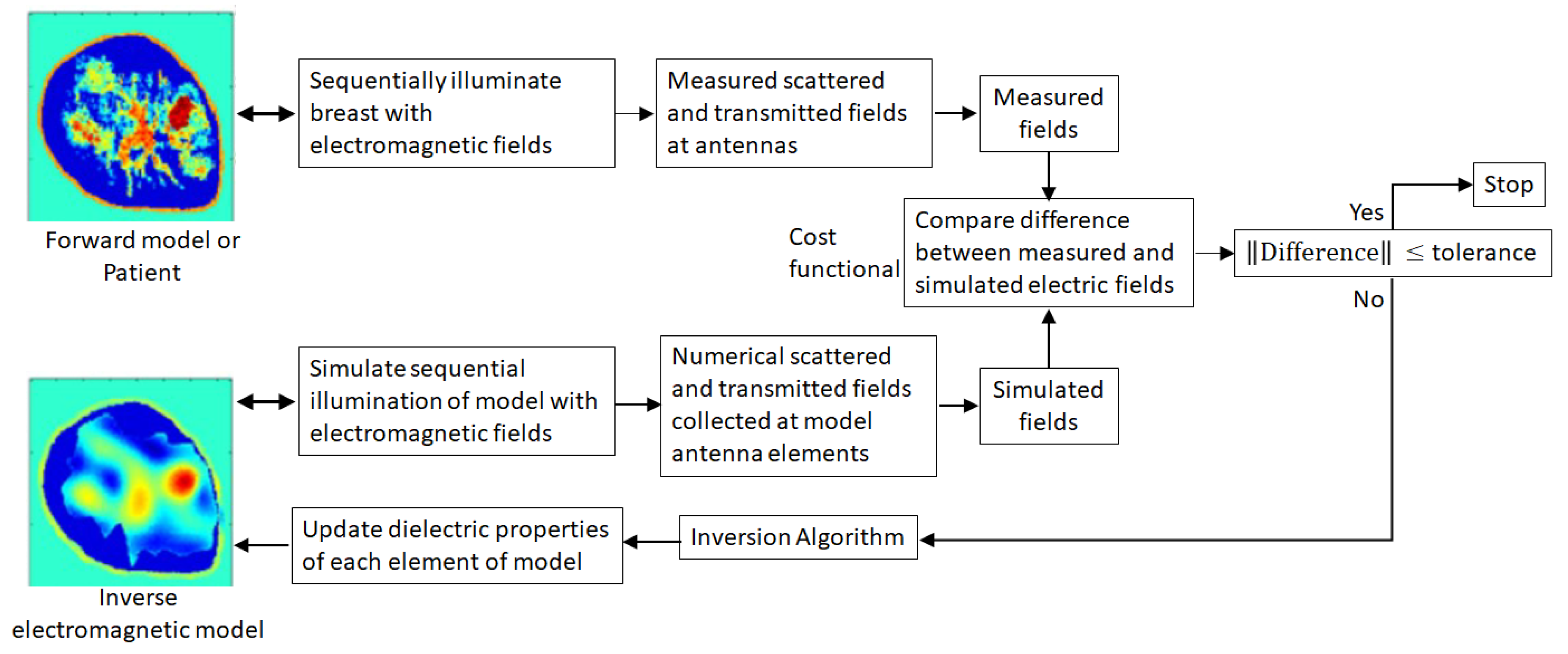
Microwave breast imaging procedure. A breast (represented by a forward model for a numerical study or measurements of a patient) is successively illuminated by incident fields from different directions. Microwave tomography is a model-based modality that extracts internal tissue information from the resulting scattered and transmitted fields to iteratively reconstruct an approximation of actual spatial distribution of dielectric properties of tissues in the breast interior. Different tissue types are distinguished from each other by their characteristic dielectric properties.
Figure 1.
Microwave breast imaging procedure. A breast (represented by a forward model for a numerical study or measurements of a patient) is successively illuminated by incident fields from different directions. Microwave tomography is a model-based modality that extracts internal tissue information from the resulting scattered and transmitted fields to iteratively reconstruct an approximation of actual spatial distribution of dielectric properties of tissues in the breast interior. Different tissue types are distinguished from each other by their characteristic dielectric properties.
Figure 2.
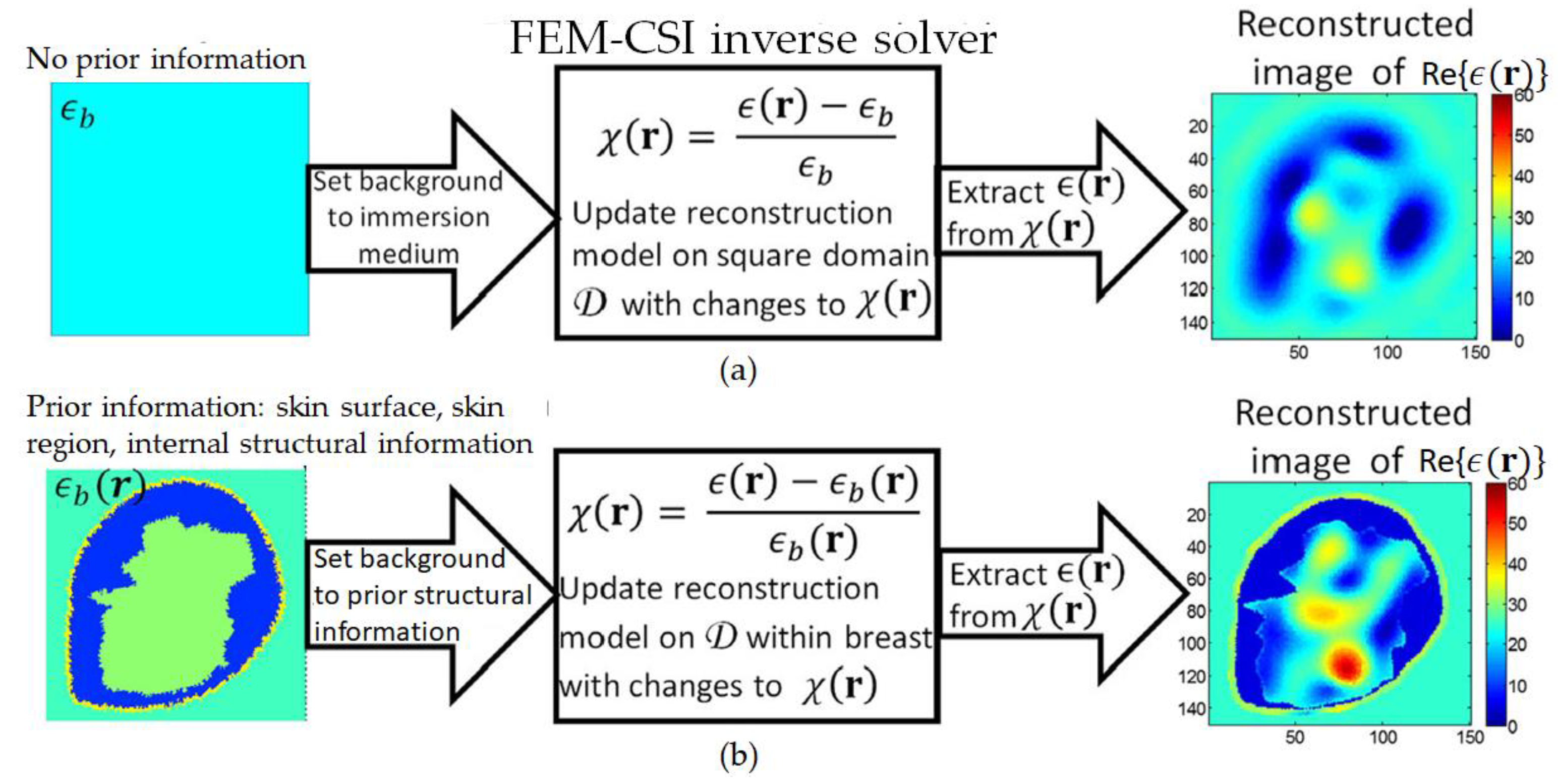
(a) With no prior information, background set to immersion medium dielectric properties, and contrast profile reconstructed over square imaging domain. (b) Prior information includes skin surface, skin region, and internal structural information. By identifying the breast surface, the imaging domain is constrained to the breast interior.
Figure 2.
(a) With no prior information, background set to immersion medium dielectric properties, and contrast profile reconstructed over square imaging domain. (b) Prior information includes skin surface, skin region, and internal structural information. By identifying the breast surface, the imaging domain is constrained to the breast interior.
Figure 3.
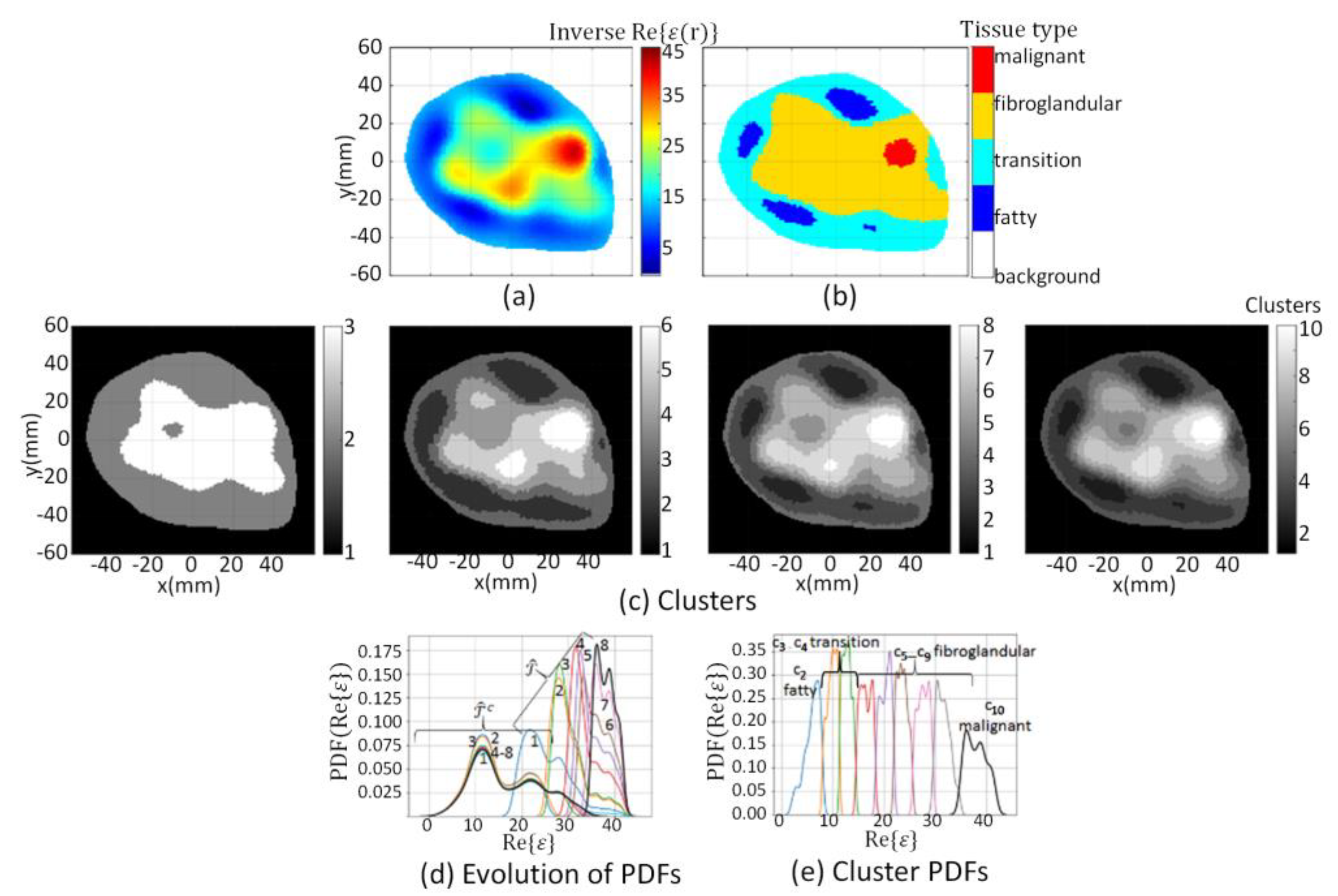
(a) Reconstructed component extracted from ; (c) Evolution of clusters at k = 3, 6, 8, and 10 when segmentation algorithm applied to ; (d) Evolution of Probability Density Function (PDF) over data within and where numbers indicate iteration; (e) PDF over data within clusters (blue line) to (black line). Cluster corresponds to fatty tissue, transition tissue, fibroglandular tissues, and corresponds to malignant tissue, which are mapped to segmentation masks leading to tissue type image (b).
Figure 3.
(a) Reconstructed component extracted from ; (c) Evolution of clusters at k = 3, 6, 8, and 10 when segmentation algorithm applied to ; (d) Evolution of Probability Density Function (PDF) over data within and where numbers indicate iteration; (e) PDF over data within clusters (blue line) to (black line). Cluster corresponds to fatty tissue, transition tissue, fibroglandular tissues, and corresponds to malignant tissue, which are mapped to segmentation masks leading to tissue type image (b).
Figure 4.
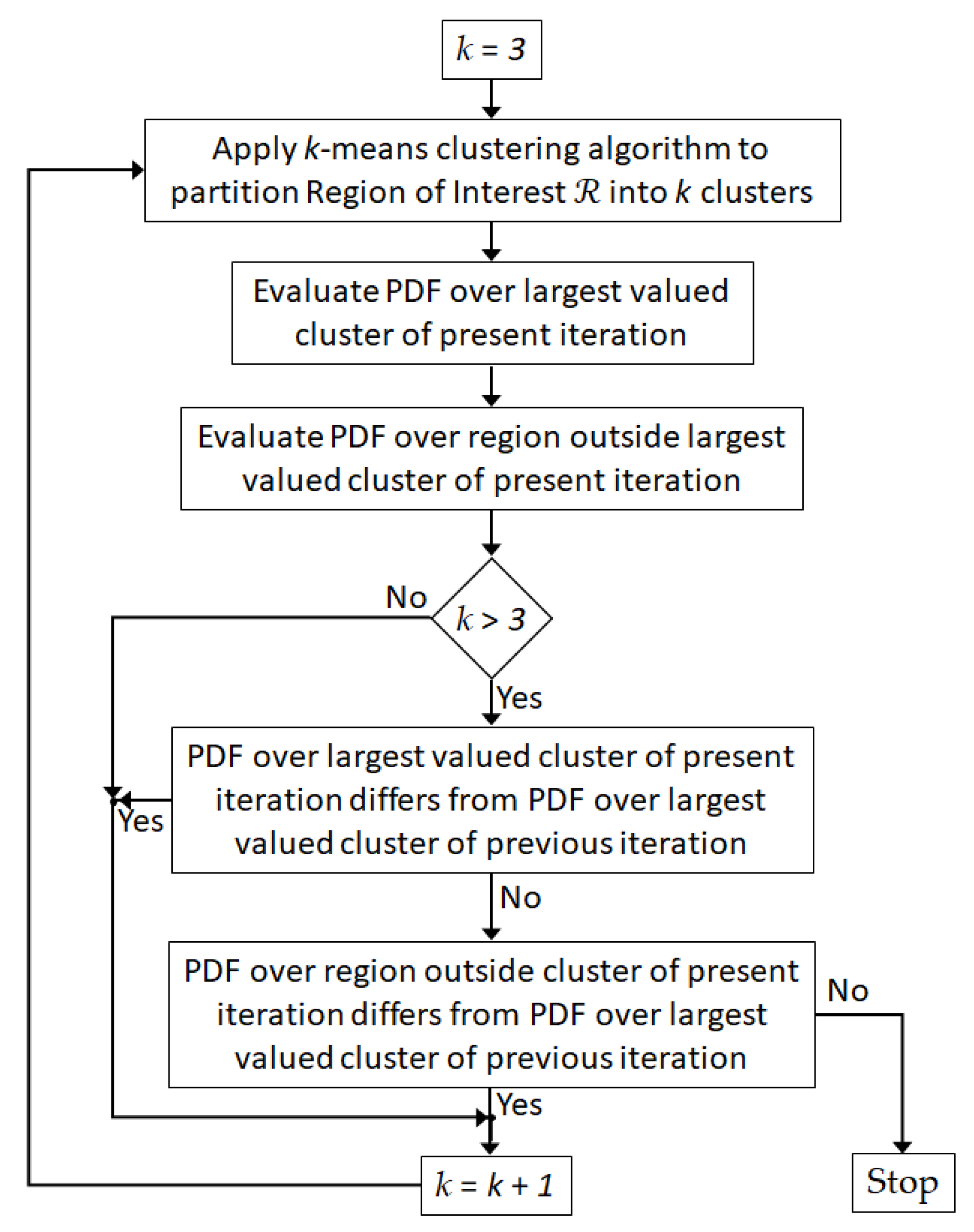
Flow diagram of segmentation algorithm used to refine partitioning of breast interior.
Figure 4.
Flow diagram of segmentation algorithm used to refine partitioning of breast interior.
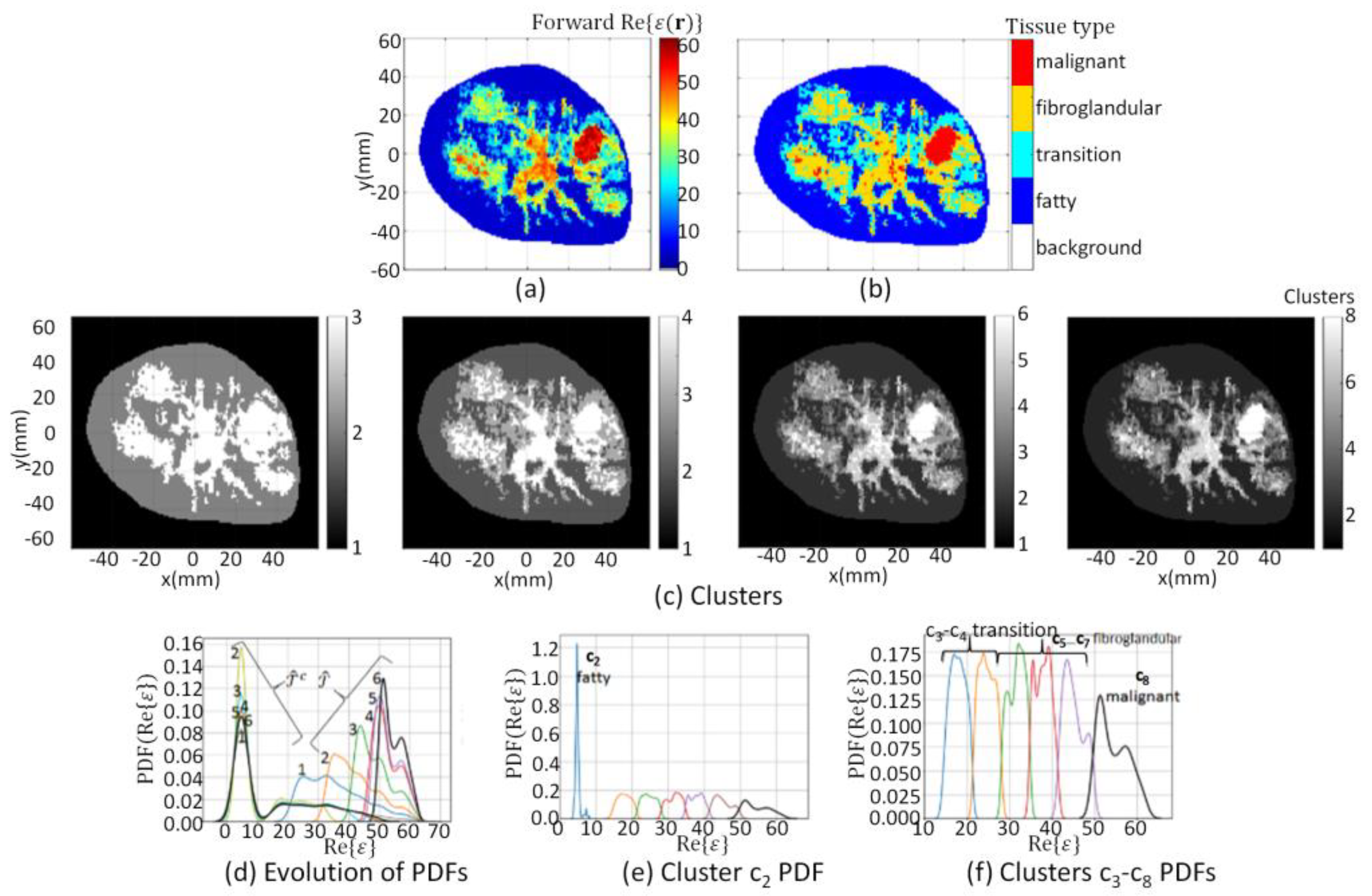
Figure 5.
Model 1 forward model segmentation results. (a) extracted from forward model; (c) Evolution of clusters at k = 3, 4, 6, and 8; (d) Evolution of PDF over data within and where numbers indicate iteration; (e) PDF over data within cluster , and (f) clusters (blue line) to (black line). Cluster corresponds to fatty tissue, corresponds to transition tissue, fibroglandular tissues, and corresponds to malignant tissue, which are mapped to segmentation masks leading to tissue type image (b).
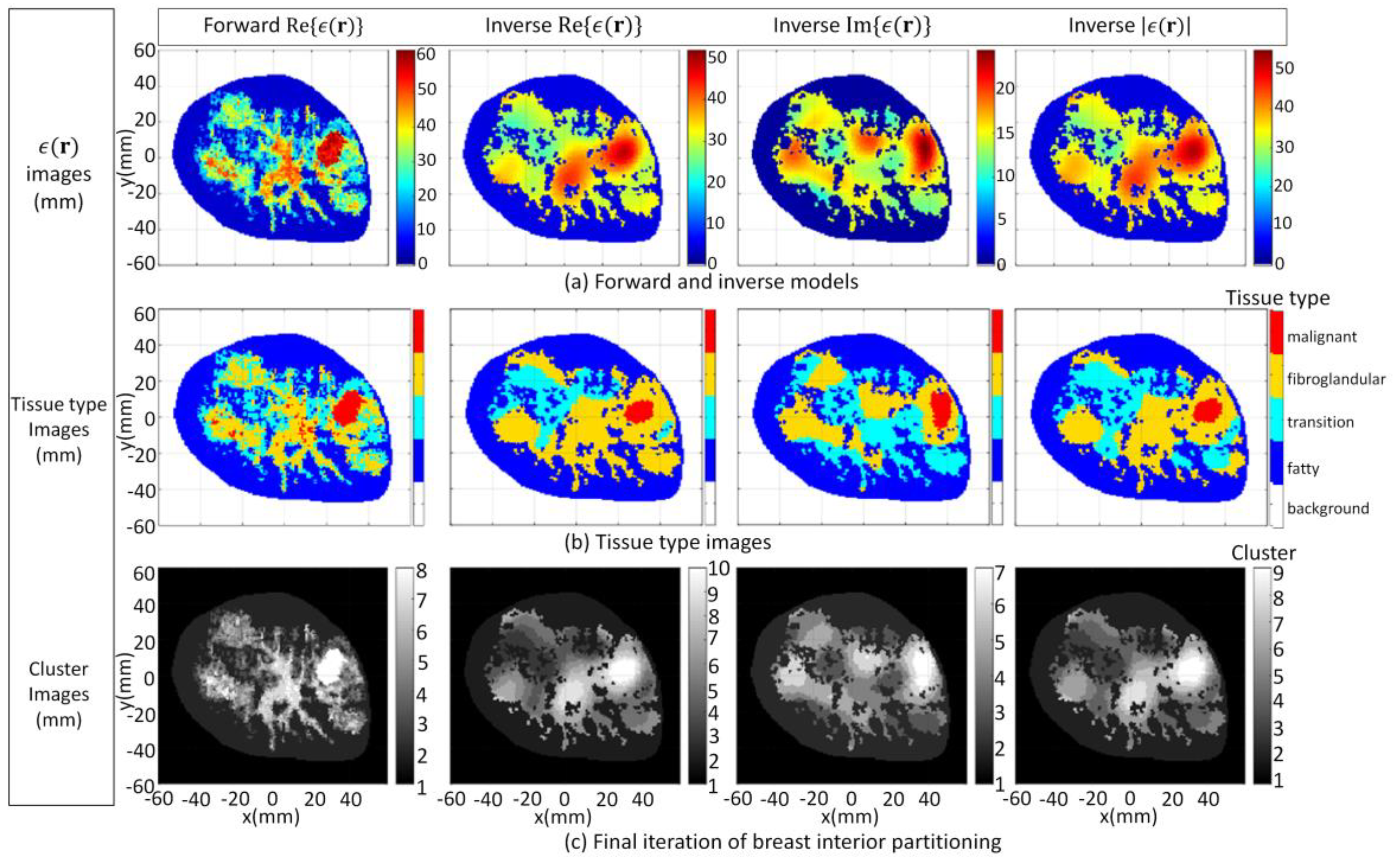
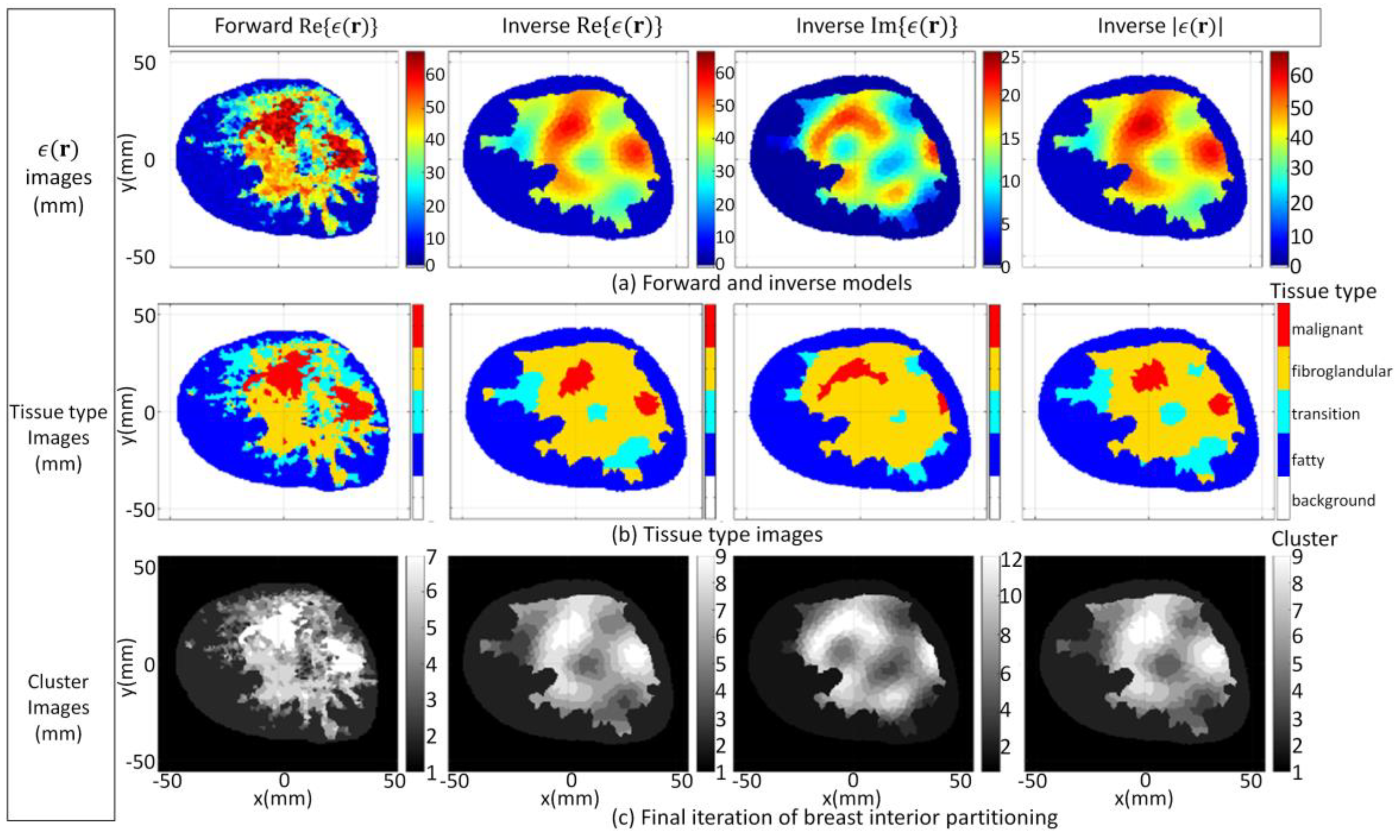
Figure 6.
Case 3.1a forward model and reconstruction results when algorithm applied to model 1 data and ϵb(r) is set to detailed internal structure (a); Tissue type images (b); Final iteration of segmentation algorithm (c).
Figure 6.
Case 3.1a forward model and reconstruction results when algorithm applied to model 1 data and ϵb(r) is set to detailed internal structure (a); Tissue type images (b); Final iteration of segmentation algorithm (c).
Figure 7.
Case 3.1b reconstruction results when algorithm applied to model 1 data and ϵb(r) is set to structural information related to skin, fat, and glandular regions extracted by radar-based technique (a); Tissue type images (b); Final iteration of segmentation algorithm (c).
Figure 7.
Case 3.1b reconstruction results when algorithm applied to model 1 data and ϵb(r) is set to structural information related to skin, fat, and glandular regions extracted by radar-based technique (a); Tissue type images (b); Final iteration of segmentation algorithm (c).
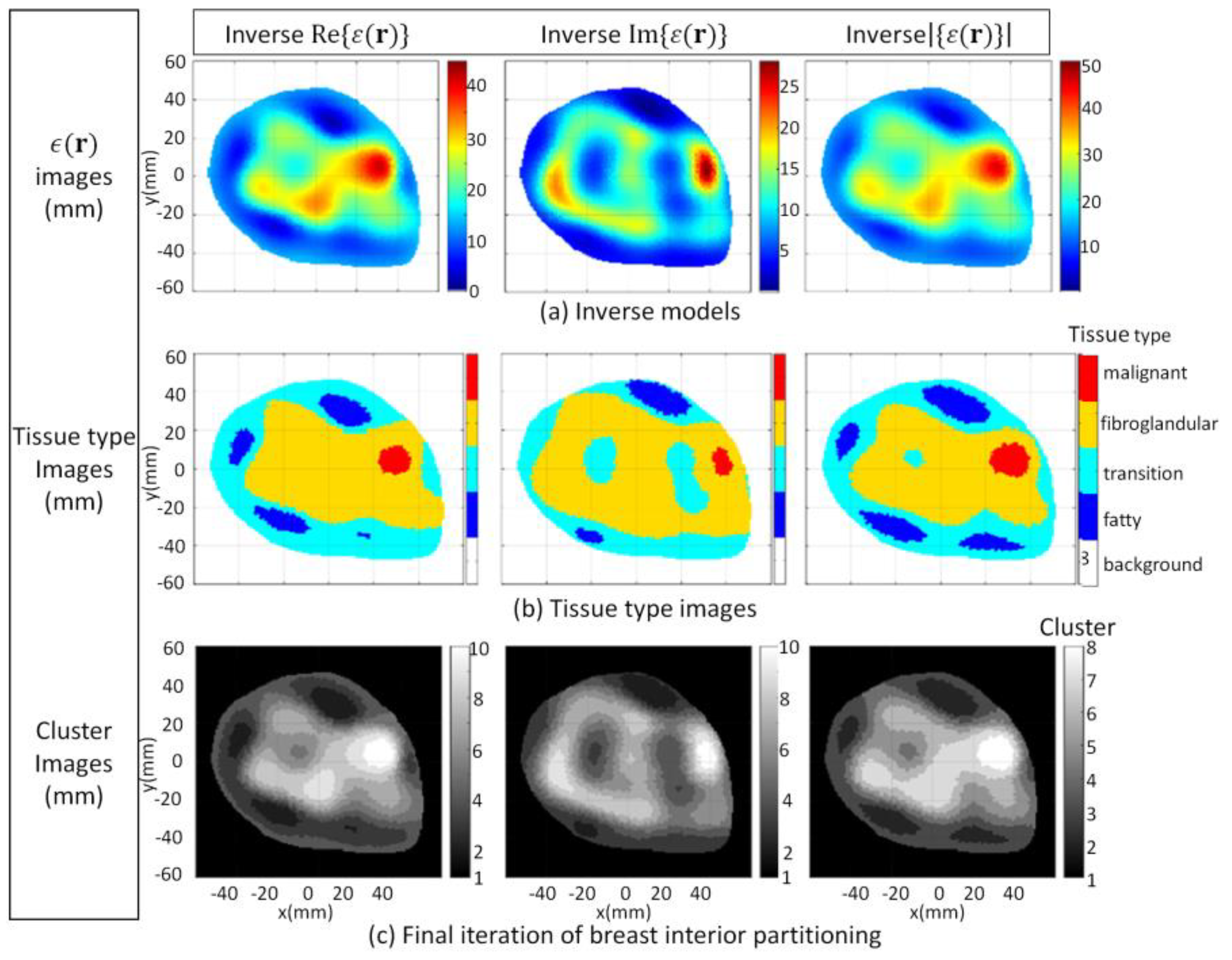
Figure 8.
Case 3.1c reconstruction results when algorithm applied to model 1 data and ϵb(r) is set to structural information related to skin region extracted by radar-based technique (a); Tissue type images (b); Final iteration of segmentation algorithm (c).
Figure 8.
Case 3.1c reconstruction results when algorithm applied to model 1 data and ϵb(r) is set to structural information related to skin region extracted by radar-based technique (a); Tissue type images (b); Final iteration of segmentation algorithm (c).
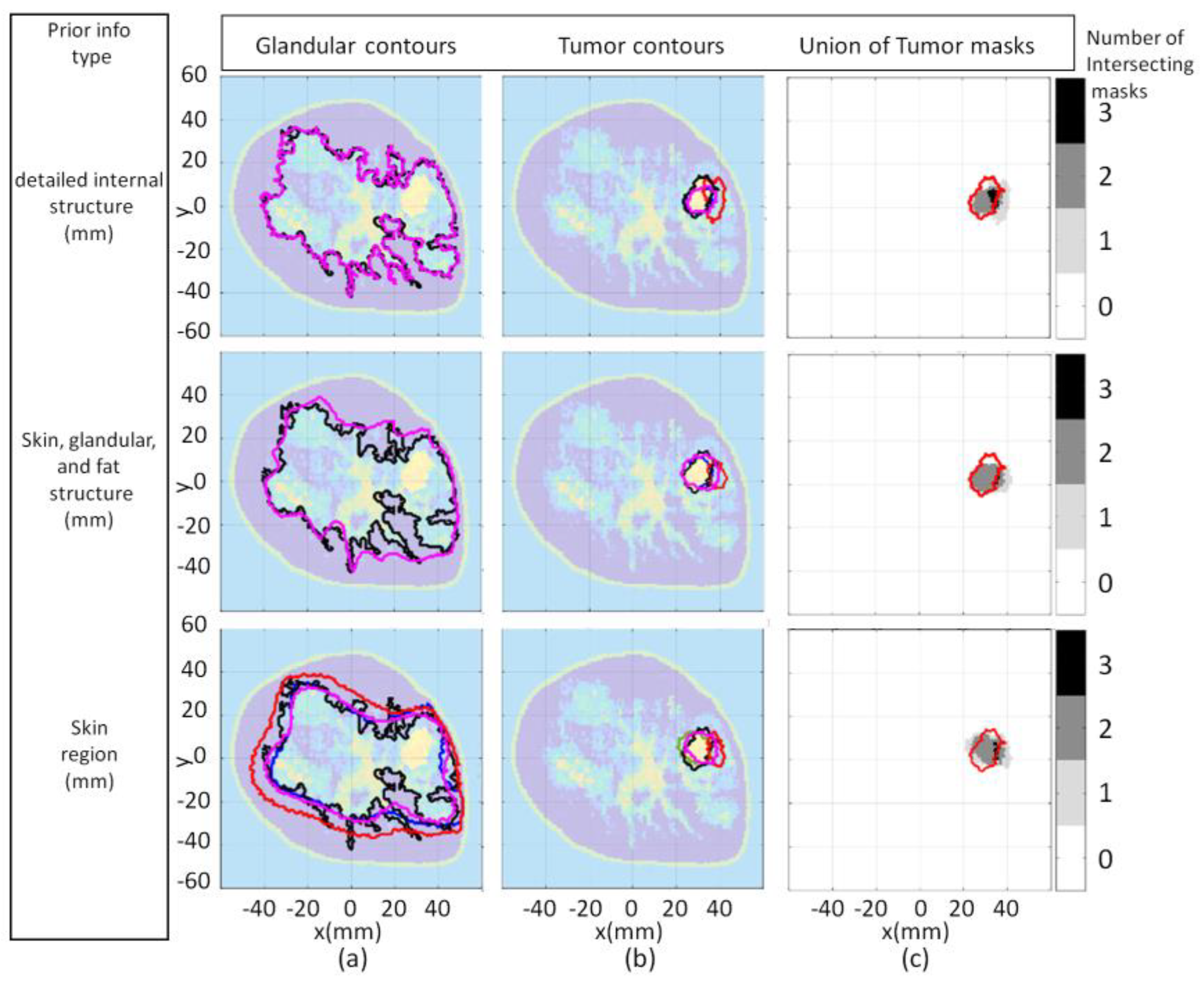
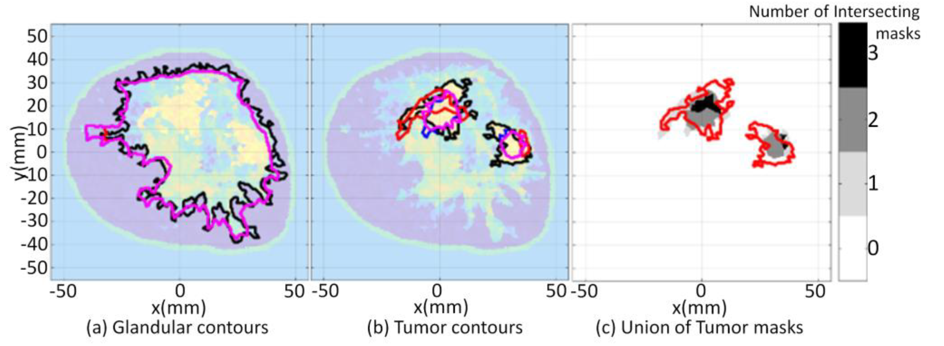
Figure 9.
Model 1 qualitative image analysis of reconstructed images formed using various prior information detail. Glandular mask contours (a), and tumor mask contours (b) with contours extracted from forward model (black-line), reconstructed (blue-line), (red-line), and (pink-line). Forward model contour (red-line) superimposed onto union of reconstructed tumor masks (c).
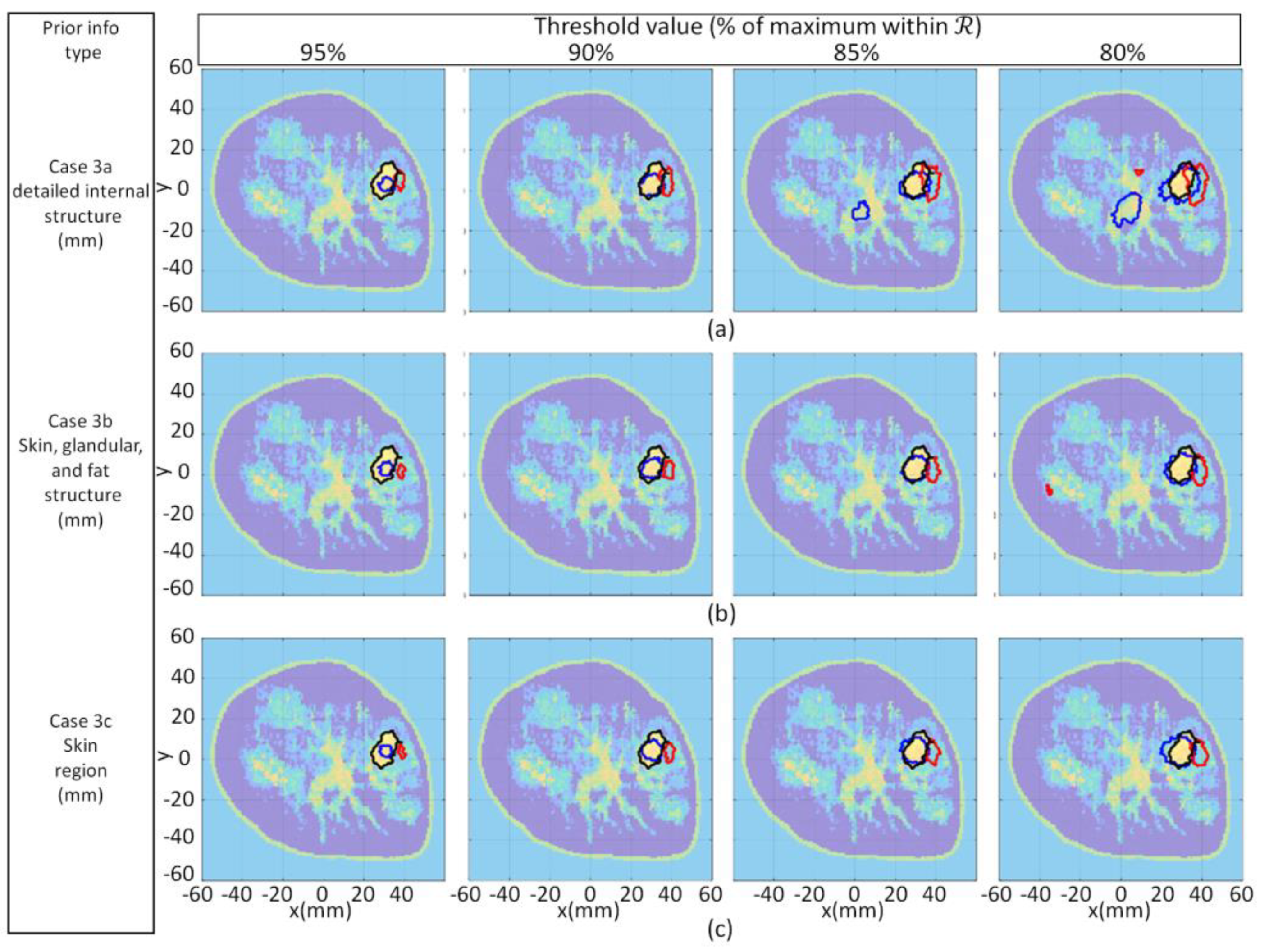
Figure 10.
Model 1 qualitative image analysis of reconstruction images using various threshold values applied to cases 3.1a (a), 3.1b (b), and 3.1c (c). For each case, contours associated with tumor masks from forward model, reconstructed Re{ϵ(r)}, and Im{ϵ(r)} shown with black, blue, and red lines, respectively, superimposed onto forward model.
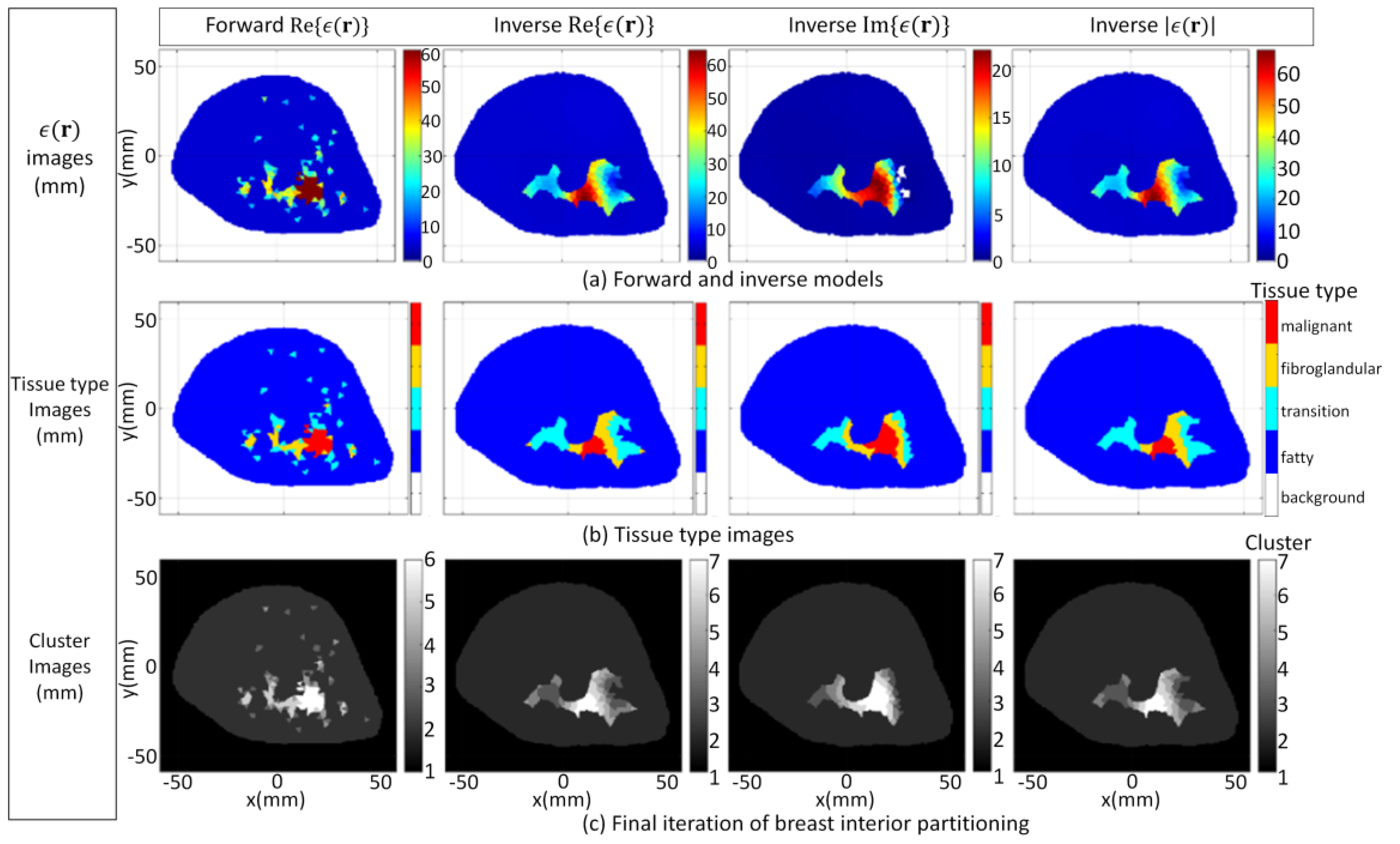
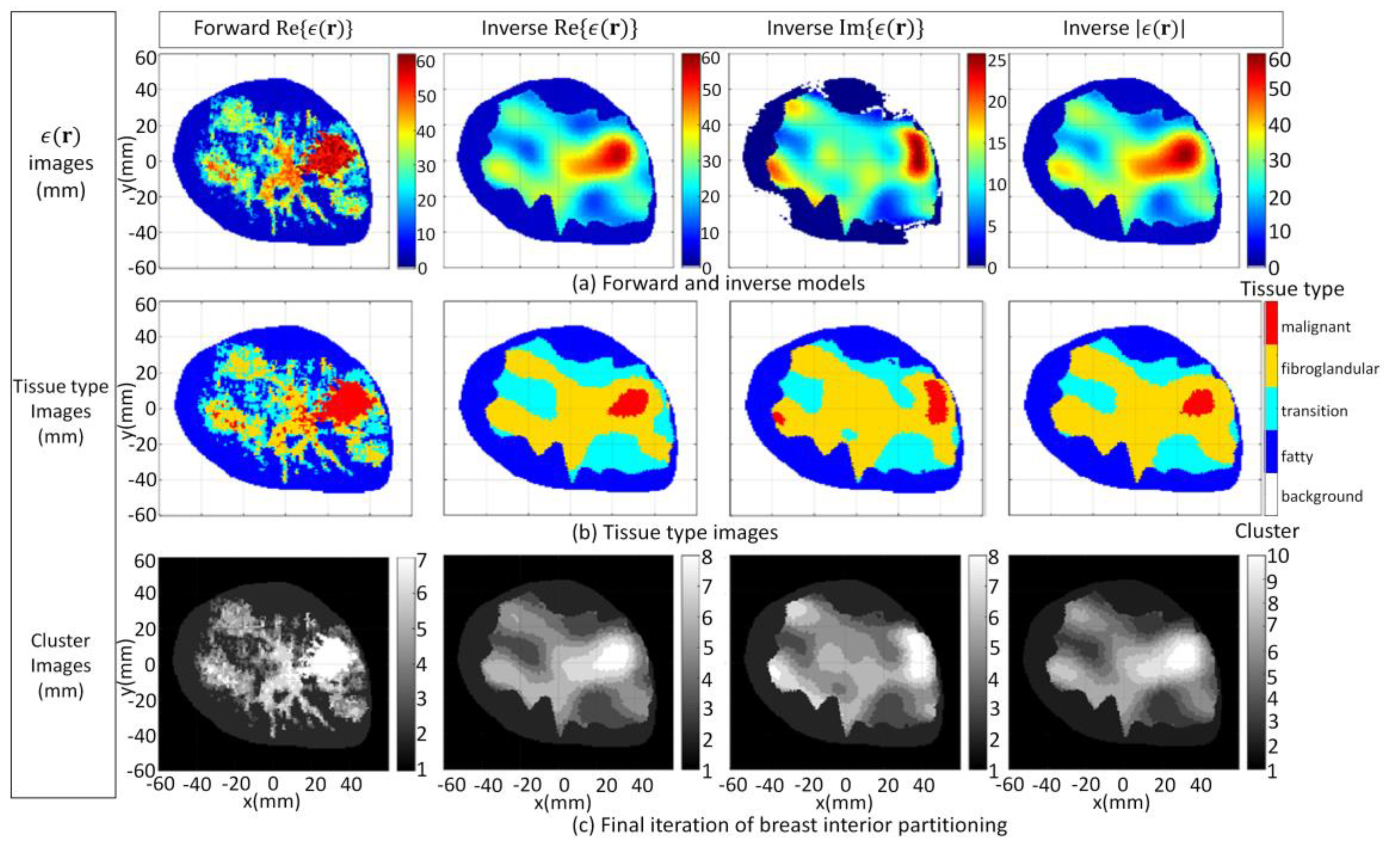
Figure 11.
Model 3.2a forward model and reconstruction results (a); Tissue type images (b); Final iteration of segmentation algorithm (c).
Figure 11.
Model 3.2a forward model and reconstruction results (a); Tissue type images (b); Final iteration of segmentation algorithm (c).
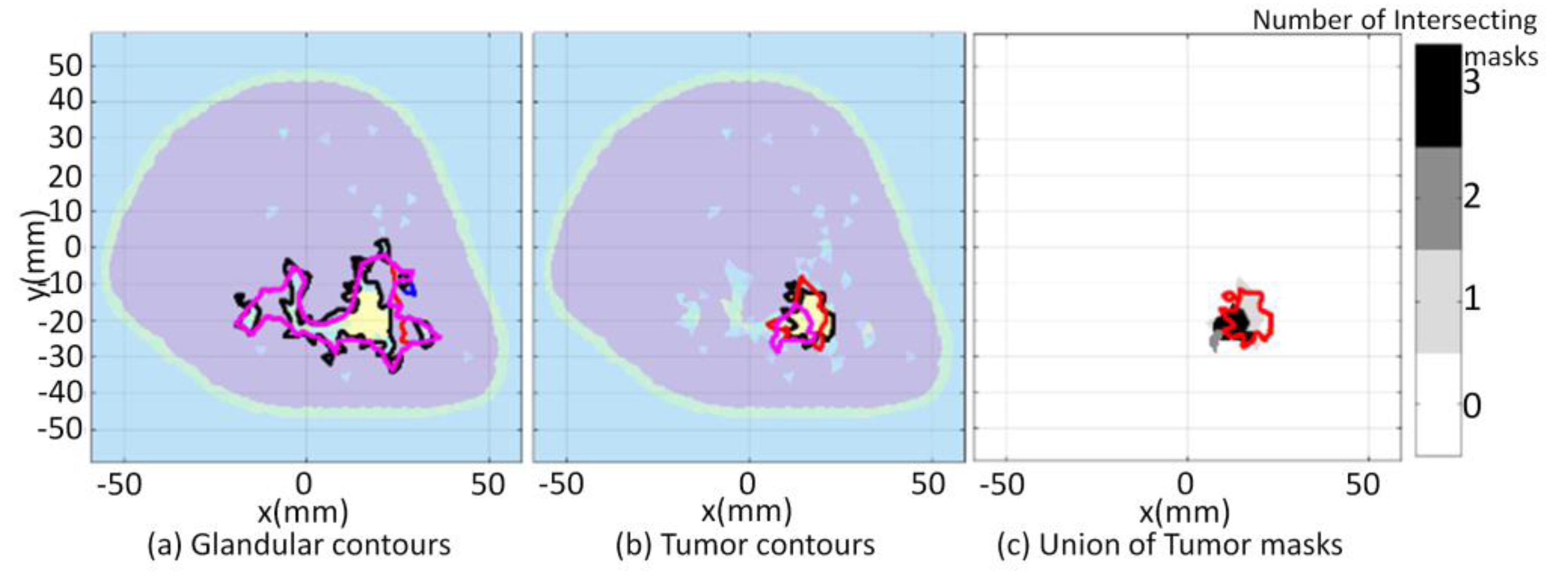
Figure 12.
Model 3.2a qualitative image analysis. Glandular mask contours (a), and tumor mask contours (b) with contours extracted from forward model (black-line), reconstructed (blue-line), (red-line), and (pink-line). Forward model contour (red line) superimposed onto union of reconstructed tumor masks (c).
Figure 13.
Model 3.2b forward model and reconstruction results (a); Tissue type images (b); Final iteration of segmentation algorithm (c).
Figure 13.
Model 3.2b forward model and reconstruction results (a); Tissue type images (b); Final iteration of segmentation algorithm (c).
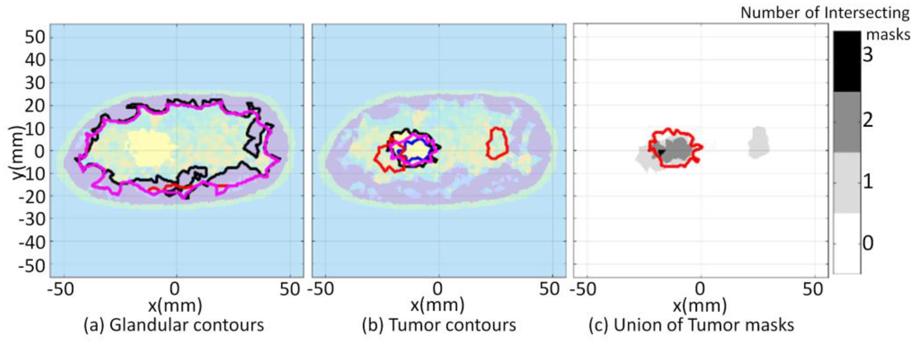
Figure 14.
Model 3.2b qualitative image analysis. Glandular mask contours (a), and tumor mask contours (b) with contours extracted from forward model (black-line), reconstructed (blue-line), (red-line), and (pink-line). Forward model contour (red line) superimposed onto union of reconstructed tumor masks (c).
Figure 15.
Model 3.2c forward model and reconstruction results (a); Tissue type images (b); Final iteration of segmentation algorithm (c).
Figure 15.
Model 3.2c forward model and reconstruction results (a); Tissue type images (b); Final iteration of segmentation algorithm (c).
Figure 16.
Model 3.2c qualitative image analysis. Glandular mask contours (a), and tumor mask contours (b) with contours extracted from forward model (black-line), reconstructed (blue-line), (red-line), and (pink-line). Forward model contour (red line) superimposed onto union of reconstructed tumor masks (c).
Figure 17.
Model 1 forward model with large tumor embedded in fibroglandular tissues and reconstruction results (a); Tissue type images (b); Final iteration of segmentation algorithm (c).
Figure 17.
Model 1 forward model with large tumor embedded in fibroglandular tissues and reconstruction results (a); Tissue type images (b); Final iteration of segmentation algorithm (c).
Figure 18.
Model 1 tumor tracking qualitative image analysis. Contours for large tumor and reduced tumor cases (a) with contours extracted from forward model (black line), reconstructed (blue line), (red line), and (pink line). Forward model contour (red line) superimposed onto union of masks formed with malignant tissue reconstructed from FEM-CSI (b).
Table 1.
Model 1: Glandular region metrics—varying degree of prior information.
Table 1.
Model 1: Glandular region metrics—varying degree of prior information.
| Case | Metric | Real | Imaginary | Magnitude |
|---|
| | Fidelity | 0.95 | 0.95 | 0.95 |
| 3.1a (detailed internal structure) | Dice | 0.95 | 0.95 | 0.95 |
| | xcorrDiel | 0.91 | 0.89 | 0.91 |
| | HA | 0.66 | 0.66 | 0.66 |
| | Fidelity | 0.85 | 0.85 | 0.85 |
| 3.1b (regional internal structure) | Dice | 0.85 | 0.85 | 0.85 |
| | xcorrDiel | 0.85 | 0.82 | 0.85 |
| | HA | 5.68 | 5.68 | 5.68 |
| | Fidelity | 0.85 | 0.81 | 0.86 |
| 3.1c (skin region) | Dice | 0.85 | 0.79 | 0.86 |
| | xcorrDiel | 0.83 | 0.75 | 0.83 |
| | HA | 4.39 | 7.09 | 4.06 |
Table 2.
Model 1: Tumor region metrics—varying degree of prior information.
Table 2.
Model 1: Tumor region metrics—varying degree of prior information.
| Case | Metric | Real | Imaginary | Magnitude |
|---|
| | RD | 0.63 | 0.20 | 0.60 |
| 3.1a (detailed internal structure) | AR | 0.95 | 0.37 | 0.87 |
| | Dice | 0.75 | 0.22 | 0.69 |
| | HA | 1.56 | 1.63 | 1.44 |
| | RD | 0.77 | 0.01 | 0.69 |
| 3.1b (regional internal structure) | AR | 0.88 | 0.65 | 0.78 |
| | Dice | 0.82 | 0.01 | 0.73 |
| | HA | 1.20 | 2.73 | 1.32 |
| | RD | 0.71 | 0.05 | 0.86 |
| 3.1c (skin region) | AR | 0.87 | 0.60 | 0.61 |
| | Dice | 0.77 | 0.06 | 0.76 |
| | HA | 1.44 | 2.42 | 1.49 |
Table 3.
Model 1 tumor region metrics: tumor region extracted with threshold technique using various values of threshold.
Table 3.
Model 1 tumor region metrics: tumor region extracted with threshold technique using various values of threshold.
| Case | Metric | 95% | 90% | 85% | 80% |
|---|
| | RD | 0.26 | 0.64 | 0.76 | 0.90 |
| 3.1a (detailed internal structure) | AR | 0.98 | 0.94 | 0.39 | −0.62 |
| Real component | Dice | 0.41 | 0.75 | 0.64 | 0.51 |
| | HA | 3.46 | 1.47 | 1.28 | 1.78 |
| | RD | 0.05 | 0.11 | 0.23 | 0.33 |
| 3.1a (detailed internal structure) | AR | 0.79 | 0.65 | 0.44 | 0.16 |
| Imaginary component | Dice | 0.07 | 0.15 | 0.26 | 0.31 |
| | HA | 3.35 | 2.28 | 1.44 | 1.48 |
| | RD | 0.26 | 0.53 | 0.72 | 0.83 |
| 3.1b (regional internal structure) | AR | 1.00 | 0.98 | 0.90 | 0.66 |
| Real component | Dice | 0.40 | 0.68 | 0.79 | 0.76 |
| | HA | 3.53 | 1.95 | 1.34 | 1.16 |
| | RD | 0.00 | 0.00 | 0.02 | 0.05 |
| 3.1b (regional internal structure) | AR | 0.86 | 0.74 | 0.61 | 0.41 |
| Imaginary component | Dice | 0.00 | 0.00 | 0.03 | 0.61 |
| | HA | 4.35 | 3.33 | 2.39 | 1.83 |
| | RD | 0.21 | 0.52 | 0.73 | 0.82 |
| 3.1c (skin region) | AR | 1.00 | 0.99 | 0.84 | 0.61 |
| Real component | Dice | 0.35 | 0.68 | 0.78 | 0.74 |
| | HA | 4.01 | 2.13 | 1.32 | 1.50 |
| | RD | 0.00 | 0.00 | 0.03 | 0.06 |
| 3.1c (skin region) | AR | 0.88 | 0.76 | 0.65 | 0.54 |
| Imaginary component | Dice | 0.00 | 0.01 | 0.04 | 0.08 |
| | HA | 4.47 | 3.41 | 2,63 | 2.11 |
Table 4.
Model 3.2a quantitative results.
Table 4.
Model 3.2a quantitative results.
| Region | Metric | Real | Imaginary | Magnitude |
|---|
| | Fidelity | 0.90 | 0.90 | 0.90 |
| Glandular | Dice | 0.90 | 0.90 | 0.90 |
| | xcorrDiel | 0.91 | 0.88 | 0.91 |
| | HA | 1.66 | 1.64 | 1.66 |
| | RD | 0.44 | 0.35 | 0.50 |
| Tumor 1 | AR | 0.92 | 0.78 | 0.96 |
| | Dice | 0.58 | 0.45 | 0.65 |
| | HA | 3.80 | 3.66 | 3.71 |
| | RD | 0.40 | 0.09 | 0.36 |
| Tumor 2 | AR | 0.94 | 0.93 | 0.94 |
| | Dice | 0.55 | 0.15 | 0.51 |
| | HA | 2.85 | 4.52 | 3.39 |
Table 5.
Model 3.2b quantitative results.
Table 5.
Model 3.2b quantitative results.
| Region | Metric | Real | Imaginary | Magnitude |
|---|
| | Fidelity | 0.61 | 0.65 | 0.62 |
| Glandular | Dice | 0.59 | 0.64 | 0.60 |
| | xcorrDiel | 0.72 | 0.79 | 0.72 |
| | HA | 3.34 | 2.54 | 3.29 |
| | RD | 0.34 | 0.76 | 0.34 |
| Tumor | AR | 0.71 | 0.61 | 0.71 |
| | Dice | 0.41 | 0.71 | 0.41 |
| | HA | 1.62 | 1.10 | 1.62 |
Table 6.
Model 3.2c quantitative results.
Table 6.
Model 3.2c quantitative results.
| Region | Metric | Real | Imaginary | Magnitude |
|---|
| | Fidelity | 0.87 | 0.88 | 0.87 |
| Glandular | Dice | 0.87 | 0.87 | 0.87 |
| | xcorrDiel | 0.92 | 0.92 | 0.92 |
| | HA | 2.13 | 2.16 | 2.13 |
| | RD | 0.37 | 0.16 | 0.69 |
| Tumor | AR | 1.00 | 0.65 | 0.95 |
| | Dice | 0.54 | 0.21 | 0.79 |
| | HA | 2.96 | 2.56 | 1.36 |
Table 7.
Model 1 tumor tracking quantitative results.
Table 7.
Model 1 tumor tracking quantitative results.
| Case | Metric | Real | Imaginary | Magnitude |
|---|
| | RD | 0.46 | 0.17 | 0.30 |
| 3.3a—Large tumor | AR | 1.00 | 0.76 | 1.00 |
| | Dice | 0.63 | 0.24 | 0.46 |
| | HA | 4.90 | 6.67 | 5.71 |
| | RD | 0.77 | 0.01 | 0.69 |
| 3.3b—Reduced tumor | AR | 0.88 | 0.65 | 0.78 |
| | Dice | 0.82 | 0.01 | 0.73 |
| | HA | 1.20 | 2.73 | 1.32 |

 and
and 


